Machine learning inversion from small-angle scattering for charged polymers
Received
24th January 2025
, Accepted 17th June 2025
First published on 23rd June 2025
Abstract
We develop Monte Carlo simulations for uniformly charged polymers and a machine learning algorithm to interpret the intra-polymer structure factor of the charged polymer system, which can be obtained from small-angle scattering experiments. The polymer is modeled as a chain of fixed-length bonds, where the connected bonds are subject to bending energy, and there is also a screened Coulomb potential for charge interaction between all joints. The bending energy is determined by the intrinsic bending stiffness, and the charge interaction depends on the interaction strength and screening length. All three contribute to the stiffness of the polymer chain and lead to longer and larger polymer conformations. The screening length also introduces a second length scale for the polymer besides the bending persistence length. To obtain the inverse mapping from the structure factor to these polymer conformation and energy-related parameters, we generate a large data set of structure factors by running simulations for a wide range of polymer energy parameters. We use principal component analysis to investigate the intra-polymer structure factors and determine the feasibility of the inversion using the nearest neighbor distance. We employ Gaussian process regression to achieve the inverse mapping and extract the characteristic parameters of polymers from the structure factor with low relative error.
1 Introduction
Semiflexible charged polymers,1 also known as polyelectrolytes,2,3 represent an essential class of materials that are fundamental to both biological processes and technological applications.4 Their unique behaviors arise from the interplay between molecular flexibility and electrostatic interactions, which are governed by the presence of ionizable groups along their chains. Notable natural examples include DNA,4,5 RNA,6 and proteins,7 all of which play pivotal roles in cellular functions. Synthetic polyelectrolytes, on the other hand, have found extensive use in a variety of fields, including water treatment,8 energy storage,9 drug delivery,10 and responsive materials.11 The conformational and dynamic properties of charged polymers are shaped by factors such as charge density, ionic strength of the surrounding environment, and the intrinsic bending stiffness of the polymer chain. A thorough understanding of these properties is crucial for tailoring polyelectrolytes to meet the specific demands of diverse applications.
To understand the structure and behavior of the charged polymers, both experimental and theoretical approaches have been employed. Experimental techniques such as small-angle scattering12 (SAS) including X-ray scattering13 and neutron scattering14,15 have proven indispensable for understanding these properties of the charged polymers.16 Scattering methods provide insights into the nanoscale structure and dynamics of charged polymers, enabling the characterization of key conformational parameters such as radius of gyration, persistence length, and inter- and intra-molecular interactions. Theoretical and computational approaches, including analytical models17,18 and computer simulations, complement experimental efforts by capturing the fundamental physics of charged polymer systems. Techniques such as molecular dynamics19,20 (MD) and Monte Carlo21,22 (MC) simulations have provided significant insights into polymer configurations, bending rigidity, and electrostatic interactions.
Despite the progress made on both the experimental and theoretical fronts, bridging the scattering function measured in SAS experiments with the polymer parameters used for modeling charged polymers in theory and simulations remains a significant challenge. The difficulties lie in extracting physical quantities about polymer conformation by decoding the scattering function. Recent advances in machine learning (ML) have opened new avenues in scattering analysis, enabling parameter extraction without requiring explicit analytical forms of the scattering function.23 By training ML models on simulation-generated data, it becomes possible to establish an inverse mapping from the scattering function to the underlying model parameters. This approach has shown promise in a variety of systems, including colloids,23–25 polymers,26–29 and lamellar structures.30,31 These applications demonstrate the potential of ML to bridge the gap between experimental scattering data and theoretical models, providing a robust framework for parameter extraction in complex systems.
In this work, we introduce such an inversion by the ML approach for the charged polymer system, where the data are generated using MC simulations. The polymer configuration is governed by the intrinsic bending stiffness, charge density and salt concentration of the surrounding medium. We first investigate the effects of these key variables on polymer conformation and then calculate the intra-polymer structure factor. To assess the feasibility of inversion, we perform principal component analysis of the scattering data and quantify the feasibility using the nearest neighbor distance of the polymer parameters in the structure factor space. Finally, we employ Gaussian process regression (GPR) to extract both the conformational and energy-related parameters of the polymers from the structure factor, demonstrating the accuracy and robustness of this approach.
2 Method
2.1 Charged polymer in an ionic fluid
We model the polymer as a chain of N connected bonds with fixed length lb, such that the joint connecting bonds i − 1 and i is ri and the tangent of bond i is ti ≡ (ri+1 − ri)/lb. The polymer energy is given by:| | 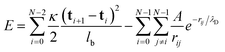 | (1) |
where κ is the bending modulus,  is the Yukawa potential, or screened Coulomb potential,20,32 that models the charge interaction, A is the interaction strength between charged monomers, λD is the Debye screening length,33 and
  is the distance between joints i and j. In addition, the self-avoidance of the polymer is enforced by adding hard sphere interaction of diameter lb between different joints. The interaction strength
  is directly related to the charge density of the polymer σe, where ε is the dielectric constant of the medium. The Debye screen length
  , where kB is the Boltzmann constant, T is the system temperature, e is elementary charge, and
  is the ionic strength, in which zi and ni are the charge number of the number density of ion species i, respectively.
2.2 Monte Carlo simulation
To calculate the conformational properties of the charged polymer at equilibrium, we sample the configuration space of the charged polymers using the off-lattice Markov Chain Monte Carlo (MCMC) method34 we previously developed; this off-lattice method provides accurate calculation of the polymer conformation and overcomes the orientational bias rooted in the lattice model.35 The polymer configuration  is updated using two MC moves: continuous crankshaft and pivot. Crankshaft picks two random joints on the polymer chain and rotates all the bonds between them for a random angle within the interval [−ϕc, ϕc]. Pivot randomly selects one joint k on the chain and rotate the preceding sub-chain (k, …, N) within a cone of angle ϕp(k) centering at the original orientation. To improve the acceptance rate of these updates and thus boost the efficiency of the simulation, the crankshaft rotation angle is adjusted according to the bending modulus such that
  , and the pivot rotation angle ϕp = ϕc. Combining these two moves allows full exploration of the polymer configuration with the contour length fixed and the polymer conformation calculated using this algorithm has been benchmarked against theoretical calculations. More details on the MCMC simulation can be found in our previous paper.34
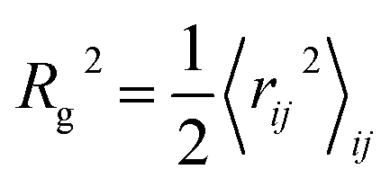
To better characterize and understand the conformation of the charged polymer, we calculate the radius of gyration, bond angle correlation and structure factor of the polymer. The radius of gyration square is  , where the 〈…〉ij denotes the average of all pair of joints. The bond–bond correlation is 〈cos(θ(s))〉 = 〈
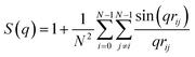
![[t with combining circumflex]](https://www.rsc.org/images/entities/b_char_0074_0302.gif) i·i+s〉i where 〈…〉i denotes the average over all bonds and s represents the contour distance between two bonds along the polymer chain. Finally, the isotropic intra-polymer structure factor12,14 is given by:
i·i+s〉i where 〈…〉i denotes the average over all bonds and s represents the contour distance between two bonds along the polymer chain. Finally, the isotropic intra-polymer structure factor12,14 is given by:
| |  | (2) |
where
q is the magnitude of the scattering vector. When running the MCMC simulation, we first randomize the system by running 2000 MC sweeps at inverse temperature
β = 1/
kBT = 0, then tempering the system for another 2000 MC sweeps while gradually decreasing the temperature to
β = 1. We sample the polymer configuration and calculate the average of the conformation parameters for while running for another 4000 MC sweeps, each MC sweep consists of
N crankshafts and
N pivot updates. We use a natural unit in our simulation where energy is in unit of
kBT = 1 and length is in unit of
lb = 1 such that the polymer contour length
L =
Nlb =
N. We use degree of discretization
L = 500 for all of our simulations.
2.3 Principal component analysis
To study the relationship between structure factor S(q) and the polymer parameters including radius of gyration Rg2, end-to-end distance R2, bending stiffness κ and interaction strength A for various screening distance λD, we generate a data set consisting of 4000 combinations of (κ, A, λD) and corresponding log![[thin space (1/6-em)]](https://www.rsc.org/images/entities/char_2009.gif) S(q) and carry out principal component analysis for the data sets. The S(q) is calculated for 100 q ∈ [10−1, 1], uniformly placed in the log scale, and κ ∼ U(5, 50), A ∼ U(0, 10) and λD ∼ Ud(1, 10), where U(a, b) is the uniform distribution in the interval [a, b] and Ud(a, b) is the discrete uniform distribution. Similar to previous work,23 we use singular value decomposition (SVD) to find the three most important bases of the 4000 × 100 matrix F = {logS(q)}, such that F = UΣVT. The diagonal entries of Σ2 are proportional to the weight of the variance of the projection of F onto each principal vector of V. Projecting F onto the first few bases provides a way to analyze F in a dimensionally reduced space. A useful tool to study the distribution of the polymer parameters Y = {(κ,A,Rg2/L2,R2/L2)} is to calculate the nearest-neighbor distance of ζ ∈ {κ,A,Rg2/L2,R2/L2} on the F manifold. For n-number of vectors, x1, x2, …, xn, the first nearest neighbor is defined as NN1(xi) = argminxj≠xi|xj − xi|; similarly, the second nearest neighbor is NN1(xi) = argminxj≠xi,NN1(xi)|xj − xi|, and we define the normalized nearest neighbor distance DNN for the ζ(x) as:
S(q) and carry out principal component analysis for the data sets. The S(q) is calculated for 100 q ∈ [10−1, 1], uniformly placed in the log scale, and κ ∼ U(5, 50), A ∼ U(0, 10) and λD ∼ Ud(1, 10), where U(a, b) is the uniform distribution in the interval [a, b] and Ud(a, b) is the discrete uniform distribution. Similar to previous work,23 we use singular value decomposition (SVD) to find the three most important bases of the 4000 × 100 matrix F = {logS(q)}, such that F = UΣVT. The diagonal entries of Σ2 are proportional to the weight of the variance of the projection of F onto each principal vector of V. Projecting F onto the first few bases provides a way to analyze F in a dimensionally reduced space. A useful tool to study the distribution of the polymer parameters Y = {(κ,A,Rg2/L2,R2/L2)} is to calculate the nearest-neighbor distance of ζ ∈ {κ,A,Rg2/L2,R2/L2} on the F manifold. For n-number of vectors, x1, x2, …, xn, the first nearest neighbor is defined as NN1(xi) = argminxj≠xi|xj − xi|; similarly, the second nearest neighbor is NN1(xi) = argminxj≠xi,NN1(xi)|xj − xi|, and we define the normalized nearest neighbor distance DNN for the ζ(x) as:| |  | (3) |
where 〈…〉x is the average overall x. The nearest-neighbor distance helps quantify the feasibility of the parameter inversion from scattering, serving as a local sensitivity metric on the scattering F manifold. By measuring how a given parameter ζ changes when moving from one scattering signature to its two closest neighbors, DNN(ζ) tells us how well small differences in logS(q) can be traced back to unique changes in ζ. Concretely, large DNN(ζ) indicates that minor variances in logS(q) can map to large jumps in ζ, signaling regions where inversion is unstable or degenerate. Whereas small DNN(ζ) means that even significant noise in logS(q) produces only modest shifts in ζ, thus the inverse mapping remains well-conditioned and robust.
2.4 Gaussian process regression
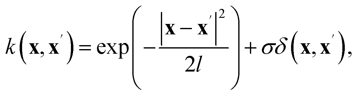
To perform inverse mapping from the scattering function, x = logS(q), to the system parameters, or inversion targets y = (κ, A, Rg/L2, R2/L2), we employ a Gaussian Process Regression (GPR) model trained on data generated through Monte Carlo (MC) simulations. Under the framework of GPR,36,37 the goal is to obtain the posterior distribution p(Y*|X*, X, Y) for the function output y. In this setup, the training and test sets are defined as X = {logS(q)}train and X* = logS(q)test, respectively, while Y and Y* correspond to the inversion targets (κ, A, Rg/L2, R2/L2). GPR assumes a Gaussian process prior over the regression function, g(x) ∼ GP(m(x), k(x, x′)), where m(x) is the prior mean function and k(x, x′) is the covariance kernel. The joint distribution for the Gaussian process is expressed as follows:| |  | (4) |
Here, we use a constant prior mean function m(x), while the kernel function is modeled as a combination of a Radial Basis Function (RBF) and a white noise term:
| |  | (5) |
where
l represents the correlation length,
σ is the variance of the observational noise, and
δ is the Kronecker delta function. These hyperparameters are optimized during training using the simulation data. In practice, we utilize the scikit-learn
38,39 Gaussian Process library due to its convenience and efficiency.
3 Results
We first study the effect of each polymer parameter on the conformation of the polymer, then investigate the scattering function of the charged polymer, where we also show the principal component analysis of our data set F = {logS(q)}. We then discuss the feasibility of inversion based on the SVD of F. With the feasibility established, we finally test our trained GPR for the inversion.
3.1 Variation of polymer conformation
Both the local bond-to-bond bending and long-range charge interaction contribute to the stiffness of the entire polymer. Such stiffness will affect the overall size of the charged polymer, which can be captured by the radius of gyration Rg2 and end-to-end distance R2. Fig. 1(a) and (c) shows both Rg2 and R2 increase with screening length λD and bending stiffness κ, and intuitively, the effects of κ on both Rg2 and R2 are more significant when λD is small, as the Rg2 and R2versus λD curves for different κ start to converge as the λD increases. In contrast, while Rg2 and R2 also increase with larger charge interaction strength A, these curves diverge as λD increases, which happens because the increasing screening length λD amplifies the effect of charge interaction.
 |
| | Fig. 1 Radius of gyration Rg2 and end-to-end distance R2 of the charged polymer versus various bending stiffness κ, charge interaction strength A and screen length λD. (a) Normalized end-to-end distance R2/L2versus screen length λD for various bending stiffness κ. (b) R2/L2versus screen length λD for various charge interaction strength A. (c) and (d), similar to (a) and (b), respectively, but for normalized radius of gyration Rg2/L2. | |
When the polymer is only subjected to bending κ, or in the case of A = 0, the polymer is a classic semiflexible polymer whose bond angle correlation can be described by a single exponential decay:
| | | 〈cosθ(s)〉 = e−s/λ0 | (6) |
where
λ0 is the persistent length.
s is the bond–bond distance along the polymer contour. However, as pointed out in a previous study,
20 the charge interaction introduces new length scales, and as a result, the bond angle correlation can be described by:
| | | 〈cosθ(s)〉 = (1 − α)e−s/λ1 + αe−s/λ2 | (7) |
λ1 and
λ2 correspond to two different length scales, and it is also notable that the effective bending rigidity can be calculated by
λe =
λ2/
α.
20
Fig. 2(a) shows the bond angle correlation function 〈cosθ(s)〉 for various screening length λD, and the fitted lines are calculated using the single scale model as in eqn (6). As λD increases, the single scale model fitting starts to diverge from the data point, indicating the necessity of switching to the double length scale model (eqn (7)); Fig. 2(b) shows such fitting results, and the two length scale model can still describe the decay of 〈cosθ(s)〉 at large λD.
 |
| | Fig. 2 Different length scales of the charged polymer, fitted using both single length scale and double length scale models. (a) Bond angle correlation 〈cosθ(s)〉 for various screening length λD with κ = 30, A = 5, solid lines are fitted using a single length scale (eqn (6)). (b) Similarly, but fitted using double length scale (eqn (7)). (c) Three persistent lengths, λ0 for the solid line, λ1 for the dashed line and λe for the dotted line, versus screening length λD for various κ with A = 5. (d) Similar to (c), but for various A with κ = 30. | |
Fig. 2(c) show all three length scales λ0, λ1 and λeversus screening length λD for various bending stiffness κ. At low λD the one length scale still fits the bond angle correlation data, and increases with increasing λD. When switching to the two length scale model, the long length scale λ1 increases with increasing λD, while the short length scale λe decreases and deviates from λ1 and then plateaus. The plateau value increases with bending stiffness κ. The switch from the one-length scale λ0 to two-length scale (λ1, λe) in the plot is determined by monitoring the divergence between the λ0 and λ1 when fitting the correlation function at low screening length λD. Fig. 2(d) shows a similar result but for various charge interaction strength A. Similar to its effect on the end-to-end distance and radius of gyration, A amplifies the effect of increasing λD, while the short length scale λe plateaus at a similar value for various A, confirming it corresponds to the bending stiffness κ.
3.2 Scattering factor of the polymers
We then turn to the inter-polymer structure factor. For comparison, we also calculate the structure factor of a solid rod, whose polymer configuration is  , with all bonds pointing to the same direction. Fig. 3(a) shows the variation of structure factor S(q) for various bending stiffness κ. Compared to the solid rod, the polymer structure factor shows a bump at a structure vector q range comparable to its radius of gyration. Fig. 3(b) shows the structure factor of the polymer divided by the rod S(q)/Srod(q), where the bump is better shown. As the bending stiffness κ increases, the peak in S(q)/Srod(q) lowers and the corresponding q value also decreases, indicating an increase of the characteristic length. Fig. 3(c) and (d) shows the S(q)/Srod(q) for various charge interaction strength A and screening length λD, and both show similar effects on the structure factor of the polymer as they make the polymer more extended and stiff.
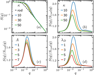 |
| | Fig. 3 Variation of the structure factor of the charged polymer. (a) Structure factor S(q) for various bending stiffness κ with λD = 3, A = 5 and rod effectively representing the κ = ∞ case. (b) Structure factor S(q) normalized by the rod's structure factor Srod(q) for various κ. (c) S(q)/Srod(q) for various charge interaction strength A with κ = 30, λD = 3. (d) S(q)/Srod(q) for various screening length λD with κ = 30, A = 5. | |
To better analyze the structure factor of the charged polymer, we carry out principal component analysis described in Sec. 2.3. By decomposing the F = {logS(q)} into F = UΣVT, we find that the singular value Σ decays rapidly versus its rank, as shown in Fig. 4(a), indicating we can represent the logS(q) ∈ F using few bases. Fig. 4(b) shows the first 3 singular vectors, and Fig. 4(c) shows the projection of a structure factor S(q) onto each basis, and the reconstruction from only the 3 bases closely matches the original S(q). This decomposition will allow us to further determine the feasibility of extracting these polymer parameters from the structure factor.
 |
| | Fig. 4 Singular value decomposition of the structure factor data set F = {logS(q)}. (a) Singular value Σ versus Singular Value Rank (SVR), with the top 3 ranks highlighted in a red circle. (b) First 3 singular vectors V0, V1 and V2. (c) Decomposition of the logS(q) with κ = 10, A = 5, and λD = 3; log(S0), log(S1) and log(S2) are projections of logS(q) onto V0, V1 and V2, respectively. | |
3.3 Feasibility for machine learning inversion
While it is straightforward to calculate the structure factor S(q) from the polymer parameters, including length L, bending stiffness κ, charge interaction strength A and screening length λD, and calculate the end-to-end distance R2 and radius of gyration Rg2 using MC simulation, the feasibility of doing the inversion is to be further assessed. Fig. 5 shows the distribution of (R2/L2,Rg2/L2,κ,A) in the structure factor space. This mapping is achieved by projecting all of the structure factor logS(q) ∈ F into the space spanned by the first 3 singular vectors (V0, V1, V2), and the corresponding 3 coefficients of each logS(q) correspond to a single point in the  space. As shown in Fig. 5(a–c), the end-to-end distance R2/L2, radius of gyration Rg2/L2 and bending stiffness κ are all well spread out on in the FV manifold, indicating they are eligible to be extracted from the structure factor. Fig. 5(d) shows the distribution of charge interaction strength A and it is unclear if it can be extracted due to some randomness in the distribution.
 |
| | Fig. 5 Distribution of the polymer parameters (R2/L2,Rg2/L2,κ,A) in the SVD space spanned by (V0, V1, V2). (a) End-to-end distance divided by length square R2/L2, (b) Radius of gyration square divided by length square Rg2/L2. (c) Bending stiffness κ. (d) Charge interaction strength A. | |
Intuitively, when then screening length λD is very small, the effect of the charge interaction becomes negligible, preventing it from having a meaningful impact on the structure factor S(q), thus it is not expected to have A feasible for extraction from the S(q) at low λD. To quantify this feasibility, we slice the structure factor data set F = {logS(q)} into different slices for different screening lengths λD, and calculate the nearest neighbor distance for each slice. As shown in Fig. 6(a), we plot 3 slices of the charge interaction strength A distribution, and the randomness reduces as the screening length λD increases. Quantitatively, Fig. 6(b) shows the nearest neighbor distance DNN for each polymer parameter and DNN(A) is much larger than that of the others when the screening length λD is small, and then it decays to lower value as the λD increases, leading to a more significant impact of the charge interaction strength A on the polymer conformation. This indicates the charge interaction strength A, which is directly related to the charge density of the polymer, is still extractable if the screening length is large enough.
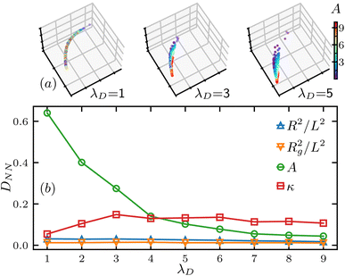 |
| | Fig. 6 Nearest neighbor distance analysis of the charge interaction strength A. (a) Value distribution of A in the SVD space for various slices of screening length λD, the axes are the same as in Fig. 5. (b) Nearest neighbor distance DNN for various polymer parameters versus different slices of the data F separated by the λD value. | |
3.4 Extraction of the polymer parameters
With the feasibility for inversion and corresponding conditions established for the polymer parameter (R2/L2,Rg2/L2,κ,A), we train the GPR using 70% of the entire data set F = {logS(q)}as the training set {logS(q)}train, and then test the trained GPR using the remaining 30% data {logS(q)}test by comparing the actual polymer parameters with the ones extracted from the structure factor S(q). The split between the training and testing data is random. To obtain the trained regressor, we need to find the optimized hyperparameters (l, σ) for each inversion target, or polymer parameters. We search for the (l, σ) that maximize the log marginal likelihood,36 which are shown in Fig. 7.
 |
| | Fig. 7 Log marginal likelihood contour of hyperparameters correlation length l and noise level σ for various polymer parameters, with the optimized value marked with a black cross. (a) End-to-end distance R2/L2. (b) Radius of gyration R2/L2. (c) Bending stiffness κ. (d) Charge interaction strength A. | |
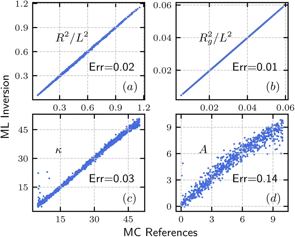
Fig. 8 shows a comparison between polymer parameters ((R2/L2,Rg2/L2,κ,A)) obtained from ML inversion and the corresponding reference used in or calculated through MC simulation. We note that due to the high nearest neighbor distance DNN(A) of charge interaction strength at low screening length λD, we only used data with λD ≥ 4 for the inversion of A. Nevertheless, the data agree well, and lie closely along the diagonal line, with relatively low error, and for polymer parameter ζ, the relative error between MC reference ζMC and ML inversion ζML is estimated by Err = 〈|ζMC − ζML|/max(ζMC,ζML)〉, where 〈…〉 is the average over all data points. The relative error is annotated on each panel of Fig. 8 and shows very high precision for ((R2/L2,Rg2/L2,κ) and good precision for A. While the errors for end-to-end distance R2, radius of gyration Rg2 and bending modulus κ are very small, the error for charge density is relatively large as we are including data with all screening length λ ≥ 4. In practice, the screening length can be estimated based on the solvent conditions; a reduced range of λD will lead to better accuracy in the extraction of charge density A.
 |
| | Fig. 8 Comparison between the polymer parameter extracted from structure factor and input or direct calculation from MC simulation. (a) End-to-end distance R2/L2. (b) Radius of gyration R2/L2. (c) Bending stiffness κ. (d) Charge interaction strength A. (a–c) Utilized all range of F and (d) only used data with λD ≥ 4. | |
4 Conclusions
In this work, we apply the off-lattice MC simulation for a semiflexible polymer to study the charged polymers, and investigate the ML inversion from scattering for such a polymer. We model the polymer using a chain of connected bonds, and the polymer energy consists of both bending energy and screened Coulomb interaction, which are proportional to the bending stiffness κ and charge interaction strength A, respectively. The charge interaction range is determined by the screen length λD. We first study the polymer conformation, where the polymer size, quantified by the end-to-end distance R2 and radius of gyration Rg2, increases with κ, A and λD. The bond angle correlation function transits from the single length scale to double length scale as the screening length λD increases. We calculate the intra-polymer structure factor S(q) of the charged polymer, compare it to that of the solid rod, and show the S(q) is sensitive to all three polymer parameters κ, A and λD. We calculate the S(q) for a wide range of κ, A and λD, then carry out principal component analysis using singular value decomposition to find the singular vectors, which allows us to do dimension reduction of the structure factor. In addition, we investigate the feasibility for inversion from scattering for both the conformation parameters: end-to-end distance R2 and radius of gyration Rg2, and the energy parameters: bending stiffness κ and charge interaction strength A. We quantify the feasibility using nearest neighbor distance DNN, and find that R2, Rg2 and κ are eligible for a wide range of screening lengths λD and the charge interaction strength A is eligible for inversion from structure factor when the λD is large enough. Finally, we use GPR to obtain the inverse mapping from structure factor S(q) to polymer parameters (R2,Rg2,κ,A) by optimizing the hyperparameters using a training data set, apply the inversion GPR to extract polymer parameters from structure factor for a test data set, and compare the ML extracted value to the MC reference; they agree well, and low relative errors are achieved.
Our approach provides a unique method to obtain the bending stiffness and the charge density σe, which is directly related to the charge interaction strength  using the scattering data. A natural next step would be to carry out a SANS experiment for some charged polymer sample, and apply our approach on the experimentally measured SANS data. In practice, this approach assumes the experimental data falls within the range of training data, and a procedure of trial and error maybe required based on the fitting results, in which the training set needs to be expanded as needed. In addition, experimental data naturally come with noise, for which a denoising procedure40 can be helpful, and the analysis of noisy data will naturally provide uncertainties by the GPR.28 Moreover, the effect of noise for the GPR prediction can be systematically studied by measuring the accuracy of the inversion when different levels of noise are added to the testing data. Finally, this framework can be expanded to the study of more complicated charged polymer systems including charge-patterned polypeptides,41 alternating copolymers42 and zwitterionic patterned polymers.43 To study these systems, it is required to model the polymer energy accordingly. It is natural to introduce variable charge interaction strength A for different monomer segments to model the charge pattern and polarity, and a screened dipole–dipole interaction can be used for modeling the zwitterionic polymer.
Data availability
The code and data for this work are available at the GitHub repository: https://github.com/ljding94/Charged_Polymer with DOI: https://doi.org/10.5281/zenodo.15624816.
Author contributions
L. D. conceived this work, carried out MC simulation and ML analysis, and drafted the manuscript. C. H. T. discussed the results and reviewed the manuscript. J. M. Y. C. conceived this work, discussed the results, and reviewed the manuscript. W. R. C. discussed the results and reviewed the manuscript. C. D. conceived this work, discussed the results and revised the manuscript.
Conflicts of interest
There are no conflicts to declare.
Acknowledgements
This research was performed at the Spallation Neutron Source and the Center for Nanophase Materials Sciences, which are DOE Office of Science User Facilities operated by Oak Ridge National Laboratory. This research was sponsored by the Laboratory Directed Research and Development Program of Oak Ridge National Laboratory, managed by UT-Battelle, LLC, for the U. S. Department of Energy. The ML aspects were supported by the U.S. Department of Energy Office of Science, Office of Basic Energy Sciences Data, and Artificial Intelligence and Machine Learning at DOE Scientific User Facilities Program under Award Number 34532. Monte Carlo simulations and computations used resources of the Oak Ridge Leadership Computing Facility, which is supported by the DOE Office of Science under Contract DE-AC05-00OR22725.
Notes and references
- R. R. Netz and D. Andelman, Phys. Rep., 2003, 380, 1–95 CrossRef CAS
 .
.
- A. V. Dobrynin and M. Rubinstein, Prog. Polym. Sci., 2005, 30, 1049–1118 CrossRef CAS .
- S. Förster and M. Schmidt, Phys. Prop. Polym., 2005, 51–133 Search PubMed .
- G. S. Manning, Q. Rev. Biophys., 1978, 11, 179–246 CrossRef CAS .
- S. Lameh, L. Ding and D. Stein, Phys. Rev. Appl., 2020, 14, 054042 CrossRef CAS .
-
V. A. Bloomfield, D. M. Crothers and I. Tinoco, Nucleic acids: Structures, properties, and functions, 2000 Search PubMed .
- C. Tanford and M. L. Huggins, J. Electrochem. Soc., 1962, 109, 98C CrossRef .
- B. Bolto and J. Gregory, Water Res., 2007, 41, 2301–2324 CrossRef CAS .
- M. Winter and R. J. Brodd, Chem. Rev., 2004, 104, 4245–4270 CrossRef CAS .
- W. B. Liechty, D. R. Kryscio, B. V. Slaughter and N. A. Peppas, Annu. Rev. Chem. Biomol. Eng., 2010, 1, 149–173 CrossRef CAS .
- M. A. C. Stuart, W. T. Huck, J. Genzer, M. Müller, C. Ober, M. Stamm, G. B. Sukhorukov, I. Szleifer, V. V. Tsukruk and M. Urban,
et al.
, Nat. Mater., 2010, 9, 101–113 CrossRef .
-
P. Lindner and T. Zemb, Neutrons, x-rays and light: scattering methods applied to soft condensed matter, 2002 Search PubMed .
- B. Chu and B. S. Hsiao, Chem. Rev., 2001, 101, 1727–1762 CrossRef CAS .
- S.-H. Chen, Annu. Rev. Phys. Chem., 1986, 37, 351–399 CrossRef CAS .
- M. Shibayama, Polym. J., 2011, 43, 18–34 CrossRef CAS .
- M. Nierlich, C. Williams, F. Boué, J. Cotton, M. Daoud, B. Famoux, G. Jannink, C. Picot, M. Moan and C. Wolff,
et al.
, J. Phys., 1979, 40, 701–704 CrossRef CAS .
- R. R. Netz and H. Orland, Eur. Phys. J. E:Soft Matter Biol. Phys., 2003, 11, 301–311 CrossRef CAS .
- A. V. Dobrynin, R. H. Colby and M. Rubinstein, Macromolecules, 1995, 28, 1859–1871 CrossRef CAS .
- M. J. Stevens and K. Kremer, J. Chem. Phys., 1995, 103, 1669–1690 CrossRef CAS .
- A. Gubarev, J.-M. Y. Carrillo and A. V. Dobrynin, Macromolecules, 2009, 42, 5851–5860 CrossRef CAS .
- F. Carlsson, P. Linse and M. Malmsten, J. Phys. Chem. B, 2001, 105, 9040–9049 CrossRef CAS .
- P. Chodanowski and S. Stoll, J. Chem. Phys., 1999, 111, 6069–6081 CrossRef CAS .
- M.-C. Chang, C.-H. Tung, S.-Y. Chang, J. M. Carrillo, Y. Wang, B. G. Sumpter, G.-R. Huang, C. Do and W.-R. Chen, Commun. Phys., 2022, 5, 46 CrossRef .
- C.-H. Tung, S.-Y. Chang, M.-C. Chang, J.-M. Carrillo, B. G. Sumpter, C. Do and W.-R. Chen, Carbon Trends, 2023, 10, 100252 CrossRef CAS .
- L. Ding, Y. Chen and C. Do, Appl. Crystallogr., 2025, 58(3), 992–999 CrossRef .
- C.-H. Tung, S.-Y. Chang, H.-L. Chen, Y. Wang, K. Hong, J. M. Carrillo, B. G. Sumpter, Y. Shinohara, C. Do and W.-R. Chen, J. Chem. Phys., 2022, 156, 131101 CrossRef CAS .
-
L. Ding, C.-H. Tung, B. G. Sumpter, W.-R. Chen and C. Do, arXiv, 2024, preprint, arXiv:2410.05574, DOI:10.48550/arXiv.2410.05574.
- L. Ding, C.-H. Tung, Z. Cao, Z. Ye, X. Gu, Y. Xia, W.-R. Chen and C. Do, Digital Discovery, 2025, 4, 1570–1577 RSC .
- L. Ding, C.-H. Tung, B. G. Sumpter, W.-R. Chen and C. Do, J. Chem. Theory Comput., 2025, 21, 4176–4182 CrossRef CAS .
- C.-H. Tung, Y.-J. Hsiao, H.-L. Chen, G.-R. Huang, L. Porcar, M.-C. Chang, J.-M. Carrillo, Y. Wang, B. G. Sumpter and Y. Shinohara,
et al.
, J. Colloid Interface Sci., 2024, 659, 739–750 CrossRef CAS .
- C.-H. Tung, L. Ding, M.-C. Chang, G.-R. Huang, L. Porcar, Y. Wang, J.-M. Y. Carrillo, B. G. Sumpter, Y. Shinohara and C. Do, J. Chem. Phys., 2025, 162, 074106 CrossRef CAS .
-
J.-P. Hansen and I. R. McDonald, Theory of Simple Liquids: with Applications to Soft Matter, Academic press, 2013 Search PubMed .
-
J. N. Israelachvili, Intermolecular and Surface Forces, Academic press, 2011 Search PubMed .
- L. Ding, C.-H. Tung, B. G. Sumpter, W.-R. Chen and C. Do, J. Chem. Theory Comput., 2024, 20, 10697–10702 CrossRef CAS .
- C.-H. Tung, L. Ding, G.-R. Huang, Y. Wang, J.-M. Y. Carrillo, B. G. Sumpter, Y. Shinohara, C. Do and W.-R. Chen, J. Chem. Phys., 2024, 161, 224107 CrossRef CAS .
-
C. K. Williams and C. E. Rasmussen, Gaussian processes for machine learning, MIT press Cambridge, MA, 2006, vol. 2 Search PubMed .
- J. Wang, Comput. Sci. Eng., 2023, 4–11 Search PubMed .
- F. Pedregosa, G. Varoquaux, A. Gramfort, V. Michel, B. Thirion, O. Grisel, M. Blondel, P. Prettenhofer, R. Weiss, V. Dubourg, J. Vanderplas, A. Passos, D. Cournapeau, M. Brucher, M. Perrot and E. Duchesnay, J. Mach. Learn. Res., 2011, 12, 2825–2830 Search PubMed .
-
L. Buitinck, G. Louppe, M. Blondel, F. Pedregosa, A. Mueller, O. Grisel, V. Niculae, P. Prettenhofer, A. Gramfort, J. Grobler, R. Layton, J. VanderPlas, A. Joly, B. Holt and G. Varoquaux, ECML PKDD Workshop: Languages for Data Mining and Machine Learning, 2013, pp. 108–122 Search PubMed .
- C.-H. Tung, S. Yip, G.-R. Huang, L. Porcar, Y. Shinohara, B. G. Sumpter, L. Ding, C. Do and W.-R. Chen, J. Colloid Interface Sci., 2025, 137554 CrossRef CAS .
- J. Dinic and M. V. Tirrell, Biomacromolecules, 2024, 25, 2838–2851 CrossRef CAS .
- C. Yi, Y. Yang and Z. Nie, J. Am. Chem. Soc., 2019, 141, 7917–7925 CrossRef CAS .
- L. Zheng, H. S. Sundaram, Z. Wei, C. Li and Z. Yuan, React. Funct. Polym., 2017, 118, 51–61 CrossRef CAS .
|
| This journal is © The Royal Society of Chemistry 2025 |
Click here to see how this site uses Cookies. View our privacy policy here. 
 Open Access Article
 This Open Access Article is licensed under a Creative Commons Attribution-Non Commercial 3.0 Unported Licence
 a,
Chi-Huan
Tung
a,
Jan-Michael Y.
Carrillo
a,
Chi-Huan
Tung
a,
Jan-Michael Y.
Carrillo

 is the Yukawa potential, or screened Coulomb potential,20,32 that models the charge interaction, A is the interaction strength between charged monomers, λD is the Debye screening length,33 and
  is the distance between joints i and j. In addition, the self-avoidance of the polymer is enforced by adding hard sphere interaction of diameter lb between different joints. The interaction strength
  is directly related to the charge density of the polymer σe, where ε is the dielectric constant of the medium. The Debye screen length
  , where kB is the Boltzmann constant, T is the system temperature, e is elementary charge, and
  is the ionic strength, in which zi and ni are the charge number of the number density of ion species i, respectively.
 is updated using two MC moves: continuous crankshaft and pivot. Crankshaft picks two random joints on the polymer chain and rotates all the bonds between them for a random angle within the interval [−ϕc, ϕc]. Pivot randomly selects one joint k on the chain and rotate the preceding sub-chain (k, …, N) within a cone of angle ϕp(k) centering at the original orientation. To improve the acceptance rate of these updates and thus boost the efficiency of the simulation, the crankshaft rotation angle is adjusted according to the bending modulus such that
 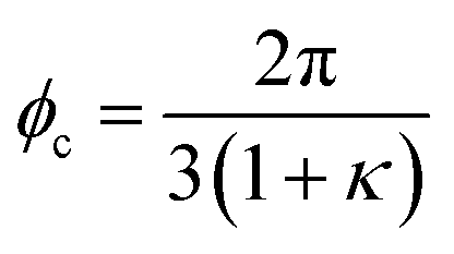 , and the pivot rotation angle ϕp = ϕc. Combining these two moves allows full exploration of the polymer configuration with the contour length fixed and the polymer conformation calculated using this algorithm has been benchmarked against theoretical calculations. More details on the MCMC simulation can be found in our previous paper.34
 , where the 〈…〉ij denotes the average of all pair of joints. The bond–bond correlation is 〈cos(θ(s))〉 = 〈


 , with all bonds pointing to the same direction. Fig. 3(a) shows the variation of structure factor S(q) for various bending stiffness κ. Compared to the solid rod, the polymer structure factor shows a bump at a structure vector q range comparable to its radius of gyration. Fig. 3(b) shows the structure factor of the polymer divided by the rod S(q)/Srod(q), where the bump is better shown. As the bending stiffness κ increases, the peak in S(q)/Srod(q) lowers and the corresponding q value also decreases, indicating an increase of the characteristic length. Fig. 3(c) and (d) shows the S(q)/Srod(q) for various charge interaction strength A and screening length λD, and both show similar effects on the structure factor of the polymer as they make the polymer more extended and stiff.


 space. As shown in Fig. 5(a–c), the end-to-end distance R2/L2, radius of gyration Rg2/L2 and bending stiffness κ are all well spread out on in the FV manifold, indicating they are eligible to be extracted from the structure factor. Fig. 5(d) shows the distribution of charge interaction strength A and it is unclear if it can be extracted due to some randomness in the distribution.


 using the scattering data. A natural next step would be to carry out a SANS experiment for some charged polymer sample, and apply our approach on the experimentally measured SANS data. In practice, this approach assumes the experimental data falls within the range of training data, and a procedure of trial and error maybe required based on the fitting results, in which the training set needs to be expanded as needed. In addition, experimental data naturally come with noise, for which a denoising procedure40 can be helpful, and the analysis of noisy data will naturally provide uncertainties by the GPR.28 Moreover, the effect of noise for the GPR prediction can be systematically studied by measuring the accuracy of the inversion when different levels of noise are added to the testing data. Finally, this framework can be expanded to the study of more complicated charged polymer systems including charge-patterned polypeptides,41 alternating copolymers42 and zwitterionic patterned polymers.43 To study these systems, it is required to model the polymer energy accordingly. It is natural to introduce variable charge interaction strength A for different monomer segments to model the charge pattern and polarity, and a screened dipole–dipole interaction can be used for modeling the zwitterionic polymer.