SurfPro – a curated database and predictive model of experimental properties of surfactants

Abstract

Despite great industrial interest, modeling the physical properties of surfactants in water based on their molecular structure remains a challenge. A significant part of this challenge is in obtaining sufficient amounts of high-quality data. Experimentally determined properties such the critical micelle concentration (CMC) and surface tension at CMC (γ_CMC) have been reported for many surfactants. However, surfactant data are scattered across many literature sources, and reported in a manner which is often unsuitable as input for predictive models. In this work, we address this limitation by compiling the SurfPro database of surfactant properties. SurfPro consists of 1624 surfactant entries curated from 223 literature sources, containing 1395 CMC values, 972 γ_CMC values and more than 657 values for Γ_max, C₂₀, π_CMC and A_min. However, only 647 structures have all reported properties, and for most surfactants multiple properties are missing. We trained a previously reported graph neural network architecture for single- and multi-property prediction on these incomplete data of all surfactant types in the database to accurately predict pCMC (−log₁₀(CMC)), γ_CMC, Γ_max and pC₂₀. We achieved state-of-the-art performance of these four properties using an ensemble of AttentiveFP models trained on ten different folds of the training data in the multi-property setting. Finally, we leveraged the predictions and uncertainties of the ensemble model to impute all missing properties for all 977 surfactants with an incomplete set of properties. We make our curated SurfPro database, proposed test split and training datasets, the imputed database, as well as our code publicly available.

---

1 Introduction

Surfactants are amphiphilic molecules that consist of a hydrophilic head and a hydrophobic tail.¹ They have a wide range of applications, including in pharmaceutical formulations, personal care, detergents and coatings.² Due to their ability to modulate surface tension at the air–water or water–oil interface and form micelles, their functions lie in controlling phenomena such as wetting, emulsification, solubilization and lubrication. The variation in surface tension γ at increasing concentrations of surfactant can be fitted to a Langmuir isotherm³ using the Szyszkowski equation.⁴ Key characteristic parameters such as the critical micelle concentration (CMC), air–water surface tension at CMC (γ_CMC), surface excess concentration (Γ_max) and the surfactant efficiency (C₂₀) can be determined from this isotherm⁵ (Fig. 1). The surface excess concentration characterises the surface concentration of surfactant molecules at the saturated surface, which measures the effectiveness of adsorption of surfactant molecules to the interface.¹ The CMC is the concentration at which the interfacial concentration of surfactant molecules is saturated and “excess” surfactant molecules self-assemble into micelles. Beyond this concentration, the surface tension is no longer sensitive to increasing surfactant concentration.¹ The C₂₀ value measures the surfactant concentration required to reduce the surface tension of a liquid by 20 mN m⁻¹.

Fig. 1 Schematic visualization of the Langmuir isotherm using the Szyszkowski equation and derived properties. Surfactant molecules adsorb to the air–water interface and lower the surface tension. With increasing surfactant concentration (x-axis, log scale) the surface tension γ (y-axis) decreases until the interface is saturated and γ stops decreasing further. Beyond this critical point, surfactants self-assemble into micelles. Surfactant properties can be extracted from this experimentally determined isotherm: the critical micelle concentration (CMC) and the surface tension at the CMC (γ_CMC). C₂₀ is defined as the surfactant concentration required to reduce the surface tension γ₀ (72 mN m⁻¹ for water at room temperature) by 20 mN m⁻¹, which quantifies the surfactant's efficiency. Γ_max represents the surface excess concentration, which is reflected in the slope of the isotherm at its steepest descent (shown in orange) and is assumed to be at γ₂₀. The area of the surfactant at the air–water interface (A_min) and the surface pressure at CMC (π_CMC) can also be determined from the isotherm (not visualized).

These parameters and other important characteristics are strongly dependent on molecular structure. As the experimental determination of surfactant properties is laborious, developing models which are capable of predicting them given only molecular structure is of high interest. For example, computational methods based on molecular dynamics (MD) simulations⁶ or descriptor-based quantitative structure–property relationship (QSPR) models⁷ have been developed to this end. Whilst these approaches predict the CMC rather accurately, MD simulations are computationally costly and QSPR models tend to perform best within a single class of surfactants (cationic, anionic, etc.).

Recently, machine learning methods have been demonstrated to be effective in predicting surfactant properties given molecular structure information as input. Qin et al.⁸ gathered a dataset of 202 experimental CMC measurements and made their dataset of SMILES strings and CMC values publicly available. The authors trained a graph convolutional neural network to predict the log(CMC) in CMC units of μM and reported an R² of 0.92/root mean squared error (RMSE) of 0.30 on their 10% test set (22 surfactants) using two graph convolutional layers (217 K parameters). The authors further demonstrated that a single model is able to accurately predict the log(CMC) for anionic, cationic, non-ionic and zwitterionic surfactants.

Moriarty et al.⁹ used the same dataset to train graph neural networks (GNN) combined with Gaussian processes, and improved upon the predictive results obtained by Qin et al.,⁸ reporting a RMSE of 0.23 using a GNN – GaussianProcesses model. The authors additionally explored another validation set of 43 surfactants¹⁰ and various GNN architecture variants. Brozos et al.¹¹ extended Qin's dataset to 429 CMC values and further collected 164 Γ_max measurements from literature to train a GNN (307 K parameters). They compared single- and multi-task learning as well as model ensembles, and achieved 0.21 mean absolute error (MAE)/0.28 RMSE for log(CMC) on a test set of 66 surfactants and 0.53 MAE/0.76 RMSE for Γ_max (24 surfactants) using a single-task model ensemble. Using the multi-task model ensemble trained on pCMC and Γ_max, they report 0.4 MAE/0.56 RMSE on Γ_max but worse performance on log(CMC) with 0.23 MAE/0.31 RMSE. In another publication the same authors further extended their database with measurements at different temperatures from literature for 492 unique surfactants and achieved accurate predictions for their test settings of 0.24 RMSE including temperature dependence.¹²

Recently, Chen et al.¹³ built upon the database of Qin et al.⁸ to a total of 779 CMC values and developed a descriptor-based QSPR model. The authors split the surfactants into two classes (ionic and non-ionic) and trained separate linear and tree-based machine learning models for both classes. They reported a MAE of 0.24/RMSE of 0.28 on a test set of 79 surfactants.

For γ_CMC, a database of 691 air–water surface tension measurements aggregated from literature was recently published by Ricardo et al.¹⁴. The authors trained a random forest model with five-fold cross validation and achieved errors of 3.38 MAE or 0.55 R² on average over five hold-out validation sets, which corresponds to the test set errors reported in other works.

Seddon et al.¹⁵ used a surface tension dataset of 154 hydrocarbon surfactants to fit the Szyszkowski equation⁴ and extract the CMC, Γ_max and Langmuir constant K_L. Using these properties, they trained QSPR models using molecular descriptors and gradient-boosted decision trees. Their approach to extract training data was restricted to the availability of γ – log(C) data, and not all surfactants in their dataset included measurements up to the CMC.

Despite these earlier studies, generally applicable surfactant property prediction models are not available. A limiting factor is the availability of a large database of experimentally determined property measurements of the CMC, γ_CMC, Γ_max and other key surfactant parameters of relevance to the design of novel systems, such as the efficiency of the surfactant in reducing the surface tension (C₂₀), the minimal area occupied by surfactants (A_min) or the surface pressure at CMC (π_CMC). Furthermore, database entries must also be suitable for modeling. For instance, providing molecular structure information in the form of machine-readable SMILES strings, as opposed to trade names or trivial names, is essential in facilitating structure-to-property models.

In this work, we address the scarcity of publicly available, machine-readable data suitable for modeling by curating a large database of surfactant properties with machine-readable structures, containing several surfactant classes and properties. This database contains CMC, γ_CMC, Γ_max, C₂₀, π_CMC and A_min values derived from experimental measurements. These data and corresponding SMILES structures were digitized and curated from 223 literature sources. For 977 out of 1624 structures not all properties have been reported, and both the fraction and distribution of reported properties differ significantly between surfactant types.

We demonstrate GNNs trained for multi-property prediction can effectively learn from this incomplete data and outperform single-property models especially for properties with the fewest data points. We leverage a stratified split to obtain a representative test set for evaluation and find an ensemble from all models trained on each cross-validation fold outperforms individual models on average. Finally, we impute all missing property values using the ensemble to complete the database. We make our curated SurfPro database, proposed test split, training data sets, imputed database and code publicly available.^16,17

2 Methods

2.1 Data acquisition

2.1.1 Dataset curation. The database was compiled by starting with a review of literature, focusing specifically on CMC. An extensive search was performed for literature reporting experimental measurements of the properties given in Table 1. We identified 223 relevant articles which reported experimental results or aggregated measurements from primary sources which originally characterized and reported the surfactant properties. A full bibliography of these articles is given in the ESI.† These articles report on data collected by several measurement methods, such as the Wilhelmy plate,^18–20 Du Noüy ring^20–22 and conductivity,²³ spanning a number of decades (1959 (ref. 24)–2021 (ref. 25)).

Table 1 Micellization-related properties of interest of surfactants, and their derivation from the experimentally determined Langmuir isotherm measuring the air–water surface tension γ at a given surfactant concentration (log(C)). All calculations are based on SI units. Abbreviations: γ₀, surface tension of water; n, 1 + number of counter ions brought to the interface (1 for non-ionic/zwitterionic, 2 for cationic/anionic, 3 for gemini); R, ideal gas constant; T, temperature in Kelvin; N_A, Avogadro constant; pCMC = –log₁₀(CMC); C₂₀ = 10^−pC₂₀

Property	Database name	Name	Unit	Calculation
CMC	CMC|pCMC	Critical micelle concentration	M|– log10(M)
γCMC	AW_ST_CMC	(Air–water) surface tension at CMC	mN m^−1
Γmax	Gamma_max	(Maximum) surface excess concentration	mol m^−2
C20	C20|pC20	Adsorption efficiency	M|– log10(M)
πCMC	Pi_CMC	Surface pressure at CMC	mN m^−1	πCMC = γ0 – γCMC
Amin	Area_min	Area at the air–water interface	nm^2

---

The results from these papers were compiled into a comprehensive database by manually digitizing and verifying the entries. Tables of property measurements reported in primary literature sources were extracted first into a comma-separated value format, alongside the chemical identifiers used to refer to the surfactants in the paper. The reported units were also extracted and converted to standardized units (Table 1). Measurements performed in the presence of any oil (e.g. paraffin) were not included the database.

A significant challenge during this phase was to generate SMILES strings²⁶ from the source formats. Many primary sources only report trivial compound names, structure images, abbreviations or “code names” defined in the manuscript text. Trivial names were mapped to SMILES strings using PubChem²⁷ searches where possible, and other structural references were transcribed manually. In some cases it was possible to efficiently translate from structured identifiers which were constructed according to a well-defined scheme of structural units. For example, in one publication²⁸ gemini surfactants were encoded as sequences of tokens encoding the head, tail, and spacer groups. In this case, it was possible to write scripts to combine SMILES fragments based on the provided identifiers into surfactant SMILES strings programmatically (results were manually verified). SMILES strings were computationally verified and canonicalized using RDKit²⁹ (version 2024.03.5). Source references are reported for each property individually, and primary sources were used where possible.

All surfactant properties reported in the database (Table 1) can be determined from experimental measurements of the relationship between surfactant concentration and air–water surface tension (Fig. 1). The shape of this plot can be reconstructed using values for CMC, γ_CMC and Γ_max, and all other reported properties can be derived from them. Properties which were calculated from other properties are annotated with a “calculated” note in the corresponding reference entry to differentiate them from entries reported in the literature.

When more than one CMC value was reported in a given source, tensiometry-based measurements (e.g. Wilhelmy plate^18–20 or Du Noüy ring^20–22), as opposed to, for example conductivity measurements,²³ were favored where possible. For duplicate entries of a given property, primary sources were prioritized over aggregated literature sources, and measurements were selected from publications with multiple reported properties over single properties for consistency between related properties. Per-property references and duplicate structures were leveraged to flag questionable entries for further manual verification. For example, entries with the same structure but significantly different experimentally reported properties and structures for which calculated properties did not match reported properties were manually verified.

2.1.2 Surfactant types. The surfactant structures were classified hierarchically into the primary classes “non-ionic”, “anionic”, “cationic” and “zwitterionic”, and the secondary classes “gemini” and “sugar-based”. Though the surfactant class is reported in most primary literature sources, classes in the database were determined based on structure by calculating the “formal charge” after removal of all counterions, and mapping this charge to the corresponding class (−3|–2 → gemini anionic, −1 → anionic, 0 → non-ionic or zwitterionic, +1 → cationic, +2|+3|+4 → gemini cationic). Zwitterionic surfactants were differentiated from non-ionic surfactants by checking for the presence of atoms with non-neutral charge in the surfactant. The “sugar-based” assignment was added manually. Algorithmically assigned surfactant types were manually verified.

2.2 Modeling

Python code used to implement, train and evaluate the models described in this section, in addition to the dataset and test split, is available on GitHub¹⁶ and Zenodo.¹⁷

2.2.1 Fingerprint-based machine learning models. Two molecular featurization approaches implemented in RDKit²⁹ combined with machine learning models were used as baselines for single-property prediction models. Extended Connectivity Fingerprints (ECFP) with 2048 bits and radius 2 were generated using “rdFingerprintGenerator.GetMorganGenerator”. RDKit topological fingerprints (RDKFP) were generated using “AllChem.RDKFingerprint”, with default hyperparameters of 2048 bits and a minimum and maximum path length of 1 and 7 bonds, respectively. These fingerprints were regressed onto properties using the “scikit-learn”³⁰ implementations (version 1.5.1) of a Random Forest Regressor (“RandomForestRegressor”, RF) and Ridge regression (“Ridge”) with default hyperparameters.

2.2.2 Graph neural network. A GNN was constructed to generate learned molecular representations from molecular graphs with node and edge features, which were then regressed onto surfactant properties. The encoder consisted of the previously reported “AttentiveFP” model,³¹ implemented in “PyTorch-Geometric”,³² which has achieved state-of-the-art performance on many property prediction tasks.^31,33,34 Molecular structures were converted into input graphs using “RDKit”²⁹ to calculate input feature vectors for every atom (39 “in_channels” features) and bond (10 “edge_dim” features) following Xiong et al.³¹ (see Table S2†). The atom (node) features are one-hot encodings of the atom's element, degree, hybridization, aromaticity and chirality, charge, number of hydrogens and radical electrons. The bond features are one-hot encodings of the bond type, its stereochemistry and whether it is part of a ring or conjugated system or not. The bond feature vector was extended with a one-hot encoding for self-loop edges. Finally, a sparse adjacency list (“edge_index”) with bidirectional edges and self-loops was constructed. The atom features, bond features and adjacency list were converted into the graph format used by “PyTorch-Geometric”.

The AttentiveFP architecture consists of multiple “message passing”³⁵ layers which refine these initial input feature vectors by propagating information based on the adjacency list. In each layer, every node's feature vector is updated by aggregating “messages” received from all adjacent nodes. AttentiveFP uses a learned message function based on the graph attention mechanism,³⁶ which is parametrized by neural networks and takes as input the feature vector of both the node, its neighbor and (optionally) their edge vector. The messages from all neighbors are aggregated into the updated node vector by a “Gated Recurrent Unit” (GRU).³⁷ Global “refinement layers” are applied after these local message passing layers, which construct a representation of the entire molecule. These attention-based layers instead connect each atom to a “virtual super node” capturing global context. The output of the encoder is a single latent vector describing the entire molecule, which is the input to the regression head. A schematic of this GNN is depicted in Fig. S1.†

2.2.3 Regression head. Latent molecular representations produced by the AttentiveFP encoder were regressed onto n_p = 1 (single-property), n_p = 3 (multi-property) or n_p = 6 (all-property) scalar property values using three sequential projections of size [d_output × 64] → [64 × 64] → [64 × n_p] with interleaved ReLU nonlinearities. LayerNormalization was applied before the first projection layer and a bias term was used for all linear layers. A mask was applied to all predictions for which no property is available in the database, which set all missing labels and affected predictions to 0 for calculation of the training loss and predictive errors.

2.2.4 GNN hyperparameter selection. AttentiveFP hyperparameter settings were screened close to the recommended defaults using a sweep of parameters. Hyperparameters for single-task and multi-task models were investigated separately. The main hyperparameter controlling the number of trainable model parameters was the “hidden dimension” of the AttentiveFP encoder, which controlled the size of the latent vector for each message passing and refinement layer. Hidden dimensions of 32, 64, 96 and 128 were used, paired with an output dimension of 64, 128, 192 and 256. Two to four message passing layers (operating at the atom level) and two to four refinement “timesteps” (operating at the graph level) with dropout probabilities of 0.0 to 0.4 were explored. These configurations yielded very small to very large models with 36 K to 635 K model parameters. Smaller models with similar accuracy to significantly larger ones were favored in these investigations. Exhaustive sweeps were performed over subsets of these configurations due to the relatively quick training times, initially with only 1 cross-validation fold, and subsequently for the better-performing configurations with 5 cross-validation folds.

These preliminary investigations on model hyperparameters indicated that the “hidden dimension” of the AttentiveFP GNN had the biggest influence on model performance. Doubling of the hidden dimension leads to a sub-quadratic increase in trainable parameters due to the linear to quadratic scaling of its constituent modules. In contrast, using more than 2 “hidden layers” and 2 “global refinement layers” significantly increases the model parameters without robust gains in performance. A “dropout” probability of p = 0.1 was found to give reliable results. Either omitting dropout or using significantly larger dropout probabilities deteriorated model performance.

Based on these investigations, we found a hidden dimension of 64 and output dimension of 128, with 2 hidden layers, 2 global refinement layers and dropout p = 0.1 consistently yielded accurate results, and used these hyperparameters for all further experiments unless stated otherwise. This configuration (AttentiveFP_64d) has 116 K model parameters including the regression head, which is significantly smaller than previously proposed GNNs for surfactants (217 K⁸ and 307 K¹¹) and molecules (586 K³⁸). A smaller variant with a hidden dimension of 32 and output dimension of 64 (AttentiveFP_32d, with a total of 36 K parameters) was also explored, as well as a larger architecture with 96 hidden dimensions and output dimension 192 (AttentiveFP_96d, 245 K parameters).

2.2.5 Multi-property prediction. Since some database properties may be calculated directly from others, “multi”-property prediction for a subset of n_p = 3 properties (pCMC, γ_CMC and Γ_max) was explored, as well as “all”-property prediction for all 6 properties outlined in Table 1. The negative log-transformed values for CMC and C₂₀ was used for all models (pCMC = –log₁₀(CMC)), and Γ_max was multiplied by 10⁶. AttentiveFP models were trained for multi- and all-property prediction using a regression head with n_p outputs, rather than training n_p separate models each with a scalar output. Due to large differences in scale for these properties, each property was scaled using the “RobustScaler” in scikit-learn³⁰ to ensure equal contributions to the loss function, which we found necessary to obtain accurate models for multi- and all-property prediction. To differentiate AttentiveFP models, we denote the hidden dimension using a subscript (e.g. AttentiveFP_64d denotes a hidden dimension size of 64) and the task (single, multi or all) in superscript, where single refers training on a single property, multi refers to training on pCMC, γ_CMC and Γ_max, and all refers to training on pCMC, γ_CMC, Γ_max, pC₂₀, A_min and π_CMC.

2.2.6 Test set split. A test set split strategy was chosen to account for the incomplete nature of the database (not all entries have a full set of properties), while allocating ∼10% of the surfactant structures and property measurements to the test set and preserving distributions of surfactant types. All measurement were included in the training and test data, regardless of the temperature they were recorded at. The test set consists of 140 surfactants and was sampled with stratification based on the surfactant type from two disjoint subsets of the database. First, stratified sampling was used to select 70 surfactants from those surfactants for which all properties have been recorded (647 surfactants). This test set was extended with 70 more surfactants, sampled with stratification from those surfactants for which only the CMC is available (632 surfactants). The surfactant classifications “anionic”, “cationic”, “non-ionic” and “zwitterionic”, “gemini cationic” and “sugar-based non-ionic” were used as a basis for stratification. Scikit-learn's “StratifiedShuffleSplit” with surfactant type as the “class label” was used to create the test set, and “StratifiedKFold” was used to obtain 10 cross-validation folds using all remaining surfactants and property measurements. The test set contains ∼10% of property measurements for CMC, Γ_max, C₂₀, A_min and π_CMC, and ∼7% of γ_CMC measurements from the database. It consists of 140 structures, with 24 anionic, 24 cationic, 52 gemini cationic, 28 non-ionic, 9 sugar-based non-ionic and 3 zwitterionic structures. Prediction errors (MAE/RMSE) for pCMC were averaged for the 140 test set structures with a pCMC measurement, while errors for γ_CMC, Γ_max and C₂₀ were calculated on the 70 test structures for which all properties are available.

2.2.7 Model training. All models were trained in sequence using PyTorch on a NVIDIA 4090 GPU with a batch size of 64 and the “AdamW” optimizer with betas 0.9 and 0.999. The HuberLoss loss criterion was chosen as the training loss, which combines the MAE and RMSE used as evaluation metrics. PyTorch Lightning's³⁹ “Trainer” was used with a learning rate initialized using the “LearningRateFinder”. Early stopping was used to terminate training after 50 epochs with no improvement in the validation MAE to avoid overfitting to the training set. All training runs stopped before the maximum number of epochs (500), most runs finished within ∼100–300 epochs in ∼25–30 minutes for all 10 models trained on 10 cross-validation splits.

2.2.8 Model performance evaluation. Test set errors were calculated using two methods. To characterise models' sensitivity to data, the “average” MAE was calculated to estimate the expected MAE value for a single model, trained on a single instance of training data (eqn (1), where K is the number of folds, N is the number of data points, y_n is a property data point and ŷ_n^k is the prediction of the property value by a model trained on the kth fold of data).

The “ensemble” MAE calculation method estimates the expected error when a prediction is made by taking the average prediction across folds (eqn (2), where K is the number of folds and ŷ^k is the prediction of a model trained on the kth fold of the data). Ensemble methods also allow model prediction uncertainty to be estimated. The standard deviation of the ensemble prediction is defined in eqn (3). Ensembles of machine learning models and (deep) neural networks have been theoretically^40,41 and empirically^42,43 shown to improve model accuracy and out-of-distribution robustness. The MAE for the ensemble prediction is given in eqn (4), with similar definitions as eqn (1).

2.2.9 Imputing missing properties. Missing experimental properties for surfactants with an incomplete set of properties were imputed using the AttentiveFP^all_64d ensemble model obtained from the 10 AttentiveFP models trained on 10 cross-validation folds. After model training, the mean of the 10 models' predictions was calculated as the ensemble prediction according to eqn (2) for all 1624 surfactant structures in the database. The standard deviation of the predictions of the 10 models was calculated following eqn (3) to quantify the uncertainty in the prediction. These predictions and uncertainties were used to impute all missing properties for 977 structures with an incomplete set of experimental properties. A standard deviation of 0.0 was assigned for measurements derived from literature values in the imputed database.

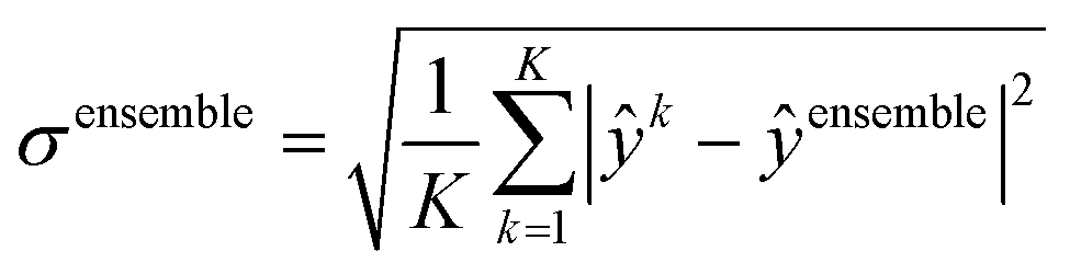3 Results and discussion

3.1 SurfPro database

Table 2 lists the overall count of experimental property measurements per property, divided by surfactant type. The largest fraction of surfactants in the database are cationic, including 904 unique structures with one (cationic) or two (gemini cationic) counter ions. The second-largest category is non-ionic, which includes 100 sugar-based surfactants, followed by anionic surfactants which contains 242 entries, and only 3 gemini anionic surfactant entries. Zwitterionic surfactants are the lowest represented class in the database, with only 54 entries overall, which includes 17 gemini zwitterionic compounds.

Table 2 Counts of experimental property measurements aggregated and curated in the SurfPro database, split by surfactant type. Properties calculated from others (Table 1) are included in these counts. They account for a small fraction of properties and are calculated based on the same Langmuir isotherm using the Szyszkowski equation

Surfactant type	SMILES	pCMC	γCMC	Γmax	pC20	Amin	πCMC	All
Cationic	316	237	274	176	176	182	195	176
Gemini cationic	588	497	416	302	308	302	326	302
Anionic	239	239	39	45	31	45	39	30
Gemini anionic	3	3	0	0	0	0	0	0
Non-ionic	325	281	145	72	71	72	101	71
Sugar-based non-ionic	100	100	74	71	71	71	74	68
Zwitterionic	36	21	24	6	0	6	9	0
Gemini zwitterionic	17	17	0	0	0	0	0	0
Total	1624	1395	972	672	657	678	744	647

---

The majority of experimental measurements (1327) were recorded between 24.85 °C to 25 °C. The properties of 55 surfactants were measured below this range (20 °C to 23 °C), and 13 surfactants were measured above it (27 °C to 40 °C). No temperature was reported for γ_CMC measurements of 228 structures obtained from Ricardo et al.,¹⁴ but the authors only included measurements at temperatures of 20 °C to 30 °C. Surfactant properties are dependent on temperature,¹² but it has also been noted that γ_CMC does not vary significantly in the temperature range 20 °C to 30 °C.¹⁴ However, we included all of the data that we collected in the test and train sets. We included data recorded outside the modal temperature range of the dataset with the aim of maximising the structural diversity, and we were unable to find data for these compounds at 25 °C. We thus expect that models trained on these data are more accurate predictors for properties at around 25 °C.

The fraction of reported properties varies significantly among surfactant types. The property pCMC has the highest number of entries in the database, with a pCMC value given for the majority of entries in each class of surfactants. The number of γ_CMC values in the data is in general the second highest for each surfactant class, and similar in proportion to the number of Γ_max, pC₂₀, A_min and π_CMC values in the database. Cationic surfactants have the highest overall proportion of micellization-related properties reported in this database. Of the 647 compounds with a complete set of reported properties, cationic and gemini cationic represent 27% and 47%, respectively. In contrast, of the 632 compounds with only CMC values reported, cationic and gemini cationic represent 7% and 28% respectively, while 30% are anionic and 28% are non-ionic.

3.2 Visualization of the distribution of reported properties by surfactant type

The distributions of experimental properties vary significantly between subsets of surfactant types, both compared to each other and compared to the full dataset (Fig. 2–5). pCMC measurements of gemini cationic structures (Fig. 2a, red) show a mean and standard deviation close to Gaussian and similar to the entire dataset (grey), while the distribution's mean shifts significantly higher for non-ionic (Fig. 2b, blue) and lower for cationic (Fig. 2c, orange) and anionic structures (Fig. 2d, green) with heavy tails. For γ_CMC the distributions of gemini cationic, cationic and non-ionic subsets (Fig. 3a–c) shift significantly relative to the entire dataset, while very few measurements are reported for anionic structures (Fig. 3d).

Fig. 2 Histograms showing the differences in distribution of pCMC for (a) gemini cationic (red), (b) cationic (orange), (c) non-ionic (blue), (d) anionic (green), with the overall distribution of the full dataset in grey. The dashed lines visualize the median of the subset (color) compared to the full dataset (grey).

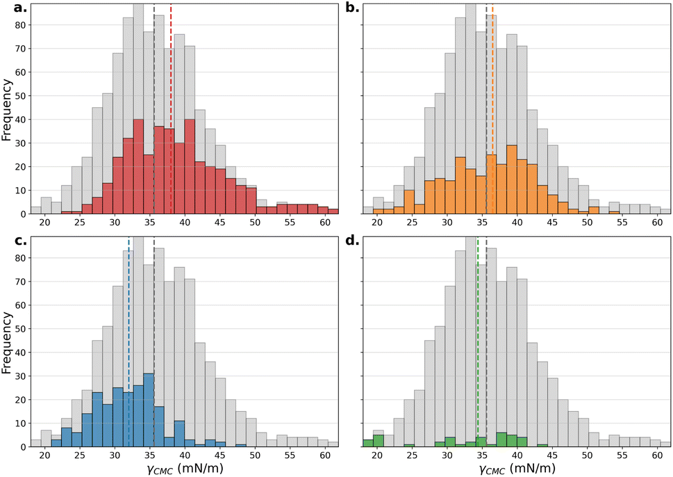Fig. 3 Histograms showing the differences in distribution of γ_CMC (mN m⁻¹) for (a) gemini cationic (red), (b) cationic (orange), (c) non-ionic (blue), (d) anionic (green), with the overall distribution of the full dataset in grey. The dashed lines visualize the median of the subset (color) compared to the full dataset (grey).

A skewed distribution is observed for Γ_max both overall and for each surfactant type (Fig. 4a–d). Heavy outliers are present in cationic structures, and a large increase of the mean Γ_max is visible for non-ionic structures. pC₂₀ measurements are normally distributed overall and for cationic and gemini cationic structures. A bi-modal distribution is observed for non-ionic (Fig. 5c) surfactants compounds, while few pC₂₀ measurements have been reported for anionic surfactants (Fig. 5d).

Fig. 4 Histograms showing the differences in distribution of Γ_max (mol m⁻² × 10⁶) for (a) gemini cationic (red), (b) cationic (orange), (c) non-ionic (blue), (d) anionic (green), with the overall distribution of the full dataset in grey. The dashed lines visualize the median of the subset (color) compared to the full dataset (grey).

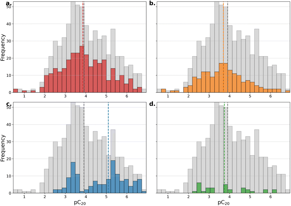Fig. 5 Histograms showing the differences in distribution of pC₂₀ for (a) gemini cationic (red), (b) cationic (orange), (c) non-ionic (blue), (d) anionic (green), with the overall distribution of the full dataset in grey. The dashed lines visualize the median of the subset (color) compared to the full dataset (grey).

3.3 Modeling results

We developed a selection of QSPR models trained to predict pCMC, γ_CMC, Γ_max, and pC₂₀. Conceptually, each model consisted of an encoder for molecular structure, and a regressor. The molecular structure encoder takes in molecular structure information in the form of a graph, and converts it into a numerical vector representation. This representation is then regressed onto molecular properties using the regressor part of the model. As “baselines”, we chose descriptors from RDKit fingerprint and ECFP-based representations, which algorithmically encode the molecular graph into vectors. ECFP and RDKit fingerprint (RDKFP) representations were regressed onto molecular properties using either random forest regression or ridge regression. GNNs have previously been shown to be effective in predicting surfactant properties.^8,9,12 Here, we selected the AttentiveFP architecture as a GNN-based encoder for molecular structure, which has previously demonstrated state-of-the-art performance on a selection of other QSPR tasks.^31,34

Distributions of properties differ between different surfactant types (Fig. 2–4). Previous reports on QSPR modeling of surfactants such as Chen et al.¹³ developed separate models for different surfactant types, while other works developed individual models capable of predicting properties for all surfactant types.^8,11 Here, we developed models which can accept any surfactant type by training on data containing surfactants of each class. The test set of 140 surfactants was selected specifically to enable evaluating models on the same set of surfactant structures for all tasks and properties. Due to the varying number of reported values for each property, ∼10% of property measurements were allocated by sampling 70 surfactants with stratification by surfactant type from two subsets of the dataset separately, respectively from structures with all reported properties, and structures with only the CMC. The distribution of surfactant type reported in the database was preserved through stratified sampling based on the surfactant type (see Methods). We included all data, regardless of the temperature they were recorded at, in training, validation and test data.

Each model was trained for three tasks: single-property, multi-property and all-property prediction. For single property prediction, models were trained to predict a single property given a molecular structure input. Multi-property AttentiveFP models were trained to simultaneously predict pCMC, γ_CMC and Γ_max. All-property AttentiveFP models were trained to simultaneously predict pCMC, γ_CMC, Γ_max, C₂₀, π_CMC and A_min. Ten-fold cross validation was used during model training. For each task and model, the MAE and RMSE were evaluated for each of 10 cross-validation folds, and averages were taken according to eqn (1). Additionally, the ensemble error (eqn (4)), corresponding to the errors of the average prediction from all models trained on each fold, was also calculated. We did not train single-task models to predict A_min or π_CMC, since they can be calculated from pCMC, γ_CMC and Γ_max. Table 3 lists all obtained predictive results for the ensemble (MAE and RMSE) for all tasks. Table S3† lists the average results for the same tasks, box plots of the results are provided in Fig. S2–S5.†

Table 3 Ensemble prediction errors for all model variants and properties under investigation. For each model, we reported the “ensemble” prediction errors obtained by first averaging the test set prediction of all 10 models for each surfactant. For the “average” prediction errors of all 10 models on the test set see Table S3. We report the mean absolute error (MAE) and root mean squared error (RMSE) for each property individually, specifically for the pCMC, γ_CMC, Γ_max × 10⁶ and pC₂₀. The best (lowest) errors for each property/metric are highlighted in bold, the second-lowest errors are italicized. See also Fig. S2–S5 for boxplot visualizations of the MAE (top) and RMSE (bottom) for all four properties

	pCMC		γCMC		Γmax × 10^6		pC20
	MAE	RMSE	MAE	RMSE	MAE	RMSE	MAE	RMSE
AttentiveFP^single32d	0.275	0.428	2.685	3.961	0.488	0.942	0.461	0.633
AttentiveFP^single64d	0.250	0.382	2.345	3.555	0.432	0.840	0.353	0.496
AttentiveFP^single96d	0.241	0.365	2.424	3.561	0.387	0.784	0.285	0.405
AttentiveFP^multi32d	0.277	0.415	2.796	3.680	0.429	0.878	—	—
AttentiveFP^multi64d	0.239	0.358	2.621	3.600	0.358	0.685	—	—
AttentiveFP^multi96d	0.237	0.360	2.308	3.407	0.333	0.573	—	—
AttentiveFP^all32d	0.279	0.419	2.711	3.626	0.479	0.999	0.349	0.530
AttentiveFP^all64d	0.246	0.358	2.548	3.516	0.353	0.842	0.282	0.390
AttentiveFP^all96d	0.235	0.346	2.591	3.531	0.347	0.707	0.259	0.363
RDKFP – Ridge	0.674	0.902	3.367	4.549	0.444	0.786	0.511	0.754
RDKFP – RF	0.630	0.840	2.939	4.211	0.443	0.773	0.582	0.743
ECFP – Ridge	0.760	1.010	3.942	5.124	0.474	0.876	0.591	0.753
ECFP – RF	0.737	0.997	4.142	5.442	0.453	0.784	0.588	0.742

---

3.3.1 ECFP and RDKit fingerprint based models. We included ECFP and RDKFP based models as “baseline” approaches in which molecular structure is encoded algorithmically, rather than learned as in the GNN approach. These models were only trained on single-property prediction tasks. All ECFP and RDKFP based approaches achieved a relatively small variance of their predictive errors, with the exception of those predicting γ_CMC. RDKit fingerprints paired with a random forest regressor (RDKFP – RF) achieved the lowest errors (MAE and RMSE) on all four properties with the exception of pC₂₀ (Fig. S2–S5,† RDKFP – Ridge – ECFP – RF). For pCMC and pC₂₀, all RDKFP based models had significantly higher MAE and RMSE (twice as large) values compared to the AttentiveFP-based models, both on average (Table S3†) and for the ensemble (Table 3). The best model of this class for pCMC prediction was RDKFP – RF, which achieved similar results for average and ensemble predictions at ∼0.63 MAE/0.84 RMSE. For Γ_max prediction, the ECFP-based approaches performed similarly to the single-task AttentiveFP models, albeit with lower variance across cross-validation folds.

3.3.2 AttentiveFP model size scaling. Fig. 6 shows MAE values obtained from different AttentiveFP model sizes for four properties and predictive tasks. The panels show the average MAE calculated across cross-validation folds, with error bars corresponding to the standard deviation, as well as MAE values derived from the ensemble prediction. The performance of the models across folds with increasing model size overlaps significantly in terms of the standard deviation. For single property prediction, there MAE decreases with increasing model size, with the exception of γ_CMC MAE increasing from AttentiveFP_64d to AttentiveFP_96d. In terms of the average error, this decrease does not appear to be significant, as there is significant overlap in terms of the standard deviation around the average MAE values. The ensemble MAE values follow a similar trend to the average MAE values, but they are much lower in magnitude, indicating that the combined prediction for a property calculated for the collection of models outperforms those of any single model. For the models trained on the multi- and all-property prediction tasks, the same trend of decreasing average MAE with increasing model size is observed. This decrease is not hugely significant due to the size of the standard deviations around the averages. As for the single property predictions, the ensemble error is much lower than the average error, but mirrors the average values' trend in model size. The results suggest that model performance increases with size, but not significantly enough to justify the use of the largest model, AttentiveFP_96d. In general, the smallest AttentiveFP_32d model always exhibits the highest average and ensemble MAE for each task and thus is not large enough to accurately fit the data for all tasks. The medium AttentiveFP_64d model achieves an accurate fit for all properties and tasks, and performs on par with the large AttentiveFP_96d model for pCMC.

Fig. 6 Comparison of AttentiveFP model size and its influence on the mean absolute error (MAE), respectively for pCMC (a), γ_CMC (b), Γ_max × 10⁶ (c) and pC₂₀ (d). The hidden dimension of the AttentiveFP model is visualized on the x-axis, which is the primary determinant of the number of trainable parameters: AttentiveFP_32d (36 K parameters), AttentiveFP_64d (116 K parameters) and AttentiveFP_96d (245 K parameters). The four panels show the four properties in the single-property (blue), multi-property (orange) and all-property (green) prediction task. The line plots with error bars visualize the average MAE and its standard deviation from the 10 models evaluated on the test set, which are slightly offset for visibility. The dashed lines visualize the ensemble MAE.

3.3.3 Model ensemble. The ensemble prediction performed significantly better than the average prediction in terms of both MAE and RMSE for every AttentiveFP-based model, across all properties, tasks and model sizes (Tables 3 and S3†). Fig. 6 shows the trends in model size discussed in the previous paragraph are nearly identical for the average (lines with error bars) and ensemble (dashed lines) MAE. Notably, for most properties and tasks the ensemble model achieved lower errors than the best individual model (Fig. S2–S5,† red stars). The ensemble prediction's significant improvement over the individual AttentiveFP model is explained by instability of the model's training⁴³ and diversity of their predictors.^40,41 The AttentiveFP models obtained from each cross-validation fold exhibit significant variance in their predictions, especially for properties with fewer data points (Fig. S3–S5†).

3.3.4 Multi-property and all-property prediction. For pCMC prediction, all AttentiveFP models (AttentiveFP_32d, AttentiveFP_64d and AttentiveFP_96d) perform similarly across the single, multi- and all-property prediction tasks for all model sizes according to the average MAE (0.31–0.35) and RMSE (0.35–0.50) (Table S3,† pCMC). This similarity in performance across training tasks is also the case for the ensemble MAE (0.24–0.28) and RMSE (0.35–0.43) (Table 3, pCMC). Thus, there is no significant improvement for pCMC prediction using multi- or all-property training strategies.

For γ_CMC prediction, according to the average error calculation metric, the MAEs of all model of the same size fall within one standard deviation of each other when trained upon the three tasks (Fig. 6). For the ensemble, single-property models perform better than multi-property models for γ_CMC prediction, except for the AttentiveFP^multi_96d model (0.33 MAE/0.57 RMSE), which outperforms both single- and all-property AttentiveFP_96d models (0.35–0.39 MAE/0.71–0.78 RMSE) (Table 3). Therefore, training on multiple or all properties is in general detrimental to predicting γ_CMC.

For Γ_max we observe more drastic improvements in performance between single-property and multi-/all-property prediction, both on average and for the ensemble (Fig. 6). For the ensemble, the single- and all-property models perform similar (0.48–0.49 MAE/0.94–1.0 RMSE) for AttentiveFP_32d, whilst the multi-property model of the same size performs better (0.43 MAE/0.88 RMSE). Increasing the model size increases the performance of the multi- and all-property models relative to the single-property model. We thus consider multi-property training to be beneficial in developing models which are better predictors of Γ_max.

Training on all properties also appears beneficial for pC₂₀ prediction. This training mode introduces a moderate increase in performance for AttentiveFP_32d according to the average metric, but this gain in performance closes as the model becomes larger. However, for the ensemble models, there is a greater difference in performance between AttentiveFP^single_32d (0.46 MAE/0.63 RMSE) and AttentiveFP^all_32d (0.35 MAE/0.53 RMSE). Again, this performance difference closes as the model size gets larger (0.29 MAE/0.41 RMSE for AttentiveFP^single_96d, 0.26 MAE/0.36 RMSE for AttentiveFP^all_96d). These results indicate that training on all properties can appreciably improve pC₂₀ prediction.

The medium (AttentiveFP_64d) and large (AttentiveFP_96d) ensemble models score similarly in the multi-property task, and differences in predictive accuracy between the multi- and all-property task are relatively small and not consistent across properties (Fig. 6 and S2–S5†). We hypothesize this is due to the similarity of information contained in both tasks, since pC₂₀, A_min and π_CMC can be calculated given pCMC, γ_CMC and Γ_max. Both multi- and all-property prediction tasks effectively contain the same information derived from the Langmuir isotherm, and therefore all derived models show comparable performance for the same model size.

3.4 Property prediction performance

3.4.1 Critical micelle concentration (pCMC). We achieved accurate predictions for our test set (140 surfactants) for pCMC using a single model for all surfactant types. All AttentiveFP model variants achieved an average MAE of 0.3–0.35/RMSE of 0.44–0.50. Furthermore, the ensemble prediction outperforms the average and almost all individual models by a significant margin, and is the best predictor across all model sizes and tasks (Fig. S2,† pCMC). The AttentiveFP_64d and AttentiveFP_96d ensembles in the multi- and all-property prediction tasks achieve state-of-the-art results with 0.24 MAE/0.35 RMSE for pCMC on the test set with all surfactant types (Table 3, pCMC). All baseline models performed poorly for pCMC prediction, with average and ensemble MAEs of 0.63 to 0.77 and RMSEs of 0.84 to 1.03. Prior work on pCMC by Brozos et al.¹¹ used GNNs and achieved a MAE of 0.21 MAE/0.28 RMSE for log₁₀(CMC) prediction in μM on 66 test set structures. Chen et al.¹³ used two separate machine learning models for ionic and non-ionic compounds, and reported a MAE of 0.24/RMSE of 0.28 on a test set of 79 surfactants.

3.4.2 Air–water surface tension (γ_CMC). We achieved accurate predictions for γ_CMC, with test set MAEs ranging between 2.31 and 3.30 mN m⁻¹ for all AttentiveFP-based models (Tables 3 and S3,† γ_CMC). These errors are significantly lower than results obtained by Ricardo et al.,¹⁴ who reported an average hold-out (test) set MAE of 3.38 mN m⁻¹ averaged over five cross-validation folds. We observe a significant variance in prediction errors for γ_CMC for all models, which affects the model averages (Fig. S3†). All but one of the fingerprint based approaches perform poorly for γ_CMC. Interestingly, the RDKFP – RF model achieves competitive accuracy with an average 3.02 MAE/4.34 RMSE on the test set, and on average performs comparably with the single-task AttentiveFP models for γ_CMC prediction. All AttentiveFP ensemble models improve upon the corresponding individual models' performance on average. The multi-property models further improve upon the results of the single-property AttentiveFP model, and the AttentiveFP^multi_96d ensemble achieves state-of-the-art performance with 2.31 MAE/3.41 RMSE (Table 3, γ_CMC).

3.4.3 Surface excess concentration (Γ_max). For Γ_max the single-task AttentiveFP models performed comparable to the fingerprint-based baseline models. The single-property AttentiveFP models achieved MAEs of 0.49 to 0.57 and RMSEs of 0.83 to 1.03, falling slightly behind all baseline models with MAEs of 0.47 to 0.50 and RMSEs of 0.80 to 0.90. The model ensembles show a small, consistent improvement for all baseline models, with more significant gains for the larger single-task ensemble models. The RDKFP – RF ensemble achieved the lowest errors among the baseline models with 0.44 MAE/0.77 RMSE, followed by the RDKFP – Ridge ensemble. Multi-property training and the model ensembles significantly improve upon the single-property models and baselines for Γ_max. The AttentiveFP^multi_96d ensemble model performed best in terms of MAE and in particular RMSE, achieving a test set error of 0.33 MAE and 0.57 RMSE (Fig. S4,† bottom). Prior work by Brozos et al.¹¹ reported a Γ_max MAE of 0.4/RMSE of 0.53 obtained from a GNN trained using multi-task learning and ensembles on a test set of 24 surfactants.

3.4.4 Surfactant efficiency (pC₂₀). For pC₂₀, all baseline approaches perform poorly (Fig. S5,† bottom). The RDKFP – Ridge ensemble achieves the lowest errors out of the machine learning models with 0.51 MAE/0.75 RMSE, but scores significantly worse than the single-property AttentiveFP models with an average 0.35 MAE/0.50 RMSE. AttentiveFP^all_96d achieves the lowest average MAE/RMSE, with the ensemble as the best overall predictor at ∼0.26 MAE/0.36 RMSE (Tables 3 and S3,† pC₂₀).

3.5 Imputing missing properties

We selected the AttentiveFP^all_64d ensemble model to provide imputed properties which complete the SurfPro dataset. For pCMC prediction the model's test MAE is 0.246, which is below the average, but approximately the median test MAE, over all AttentiveFP ensemble models.

Inspection of the model's parity plot for pCMC (Fig. S6a†) and the distribution of differences between the true and predicted values (Fig. S6b†) indicates that the model predicts pCMC for each surfactant type with similar accuracy. Therefore, the model's performance for pCMC prediction does not appear to be dependent on the surfactant type.

In the case of γ_CMC prediction, the overall test MAE is 2.55, just below the mean test MAE, and well below the median, for the AttentiveFP ensemble models. The parity plot (Fig. S7a†) and distribution of errors (Fig. S7b†) indicates that the majority of samples in each surfactant class are similarly distributed close to the mean error. However, there are some samples of the anionic, cationic and gemini surfactant classes which have significantly higher errors than average. Since these are isolated examples from the test data set, we cannot draw any inferences about any structural basis for the low prediction accuracy for these samples.

For Γ_max prediction, the test MAE is 0.35, which is below the mean (and median) test MAE for all AttentiveFP ensemble models. As for pCMC and γ_CMC, parity plots (Fig. S8a†) and distributions of errors (Fig. S8b†) indicate similar model performance over each class of surfactants. However, there is single outlier cationic surfactant sample whose Γ_max value is predicted to be significantly lower than its experimental value. Again, we cannot infer any general insight into model behaviour based on this single sample.

Finally, for pC₂₀, the model performs with a test MAE of 0.28, which is approximately the median, but above the mean test MAE over all AttentiveFP ensemble models. The pC₂₀ values for gemini surfactants are in general lower in error, as indicated by their relatively narrow distribution of errors about 0.0 compared to the other surfactant classes (Fig. S9a and b†). Thus, the AttentiveFP^all_64d model performs well in comparison to the other investigated models, performing similarly to the larger AttentiveFP^all_96d and AttentiveFP^multi_96d ensemble models, and significantly better than all smaller AttentiveFP_32d models. The model can also make predictions across variety of surfactant classes well, and in general does not appear be systematically biased to predict one surfactant class with better accuracy than any other.

Out of the 1624 structures, only 647 have all properties reported, and we fill the database with the ensemble model's predictions and uncertainties for all missing properties for those 977 structures. We used the AttentiveFP^all_64d ensemble model to calculate predictions for missing values in the database using the mean prediction of the ten members of the ensemble (eqn (2)). We also used these ten values to estimate the uncertainty of their mean prediction by calculating their standard deviation (eqn (3)). The entries for which the literature values are provided are assigned a standard deviation of 0.0 in the imputed database. The imputed database is available on Github¹⁶ and Zenodo.¹⁷

4 Conclusion

SurfPro is a manually curated surfactant property database of 1624 unique amphiphiles, which we have made publicly available for the community. At the time of writing, it is the largest dataset for this class of compounds, containing 1624 unique surfactant entries with corresponding measurements of the CMC, γ_CMC, Γ_max and C₂₀. Importantly, literature sources typically do not include experimental measurements of all properties of surfactants, often only reporting pCMC or γ_CMC values. Therefore, despite the size of the database, it remains incomplete as not all samples have a complete set of annotated properties. Furthermore, SurfPro contains only three anionic gemini surfactants, 21 cationic gemini with 3 or 4 counterions, and three high molecular weight compounds (≥2000 Da). Future data collection efforts could thus be targeted to address the balance of structural diversity and experimental surfactant property measurements to fill the chemical structure and property spaces of surfactants more efficiently.

Using the SurfPro database, we trained an ensemble of GNN-based models for single- and multi-property prediction for pCMC, γ_CMC, Γ_max and pC₂₀. This model then allowed us to impute missing property values for 977 compounds in the SurfPro database, thus providing a complete database consisting of experimentally measured properties from literature sources, and a set of estimates according to the GNN ensemble model. We hope the database and modeling strategy will provide new avenues in data-driven property prediction and surfactant design.

Data availability

The SurfPro database (“surfpro_literature.csv”), reference list (“surfpro_bibliography.bib”), “imputed” database (“surfpro_imputed.csv”), test split (“surfpro_test.csv”), cross-validation folds (“surfpro_train.csv”) and Python code used to implement, train and evaluate the models described in this work are available via GitHub (https://github.com/BigChemistry-RobotLab/SurfPro¹⁶) and Zenodo (https://zenodo.org/records/14931937, DOI: https://doi.org/10.5281/zenodo.14931937).¹⁷

Author contributions

Conceptualization – SH, LH, AP, WTSH, WER. Data curation – SH, LH, WER. Model development, training & evaluation – SH, WER. Supervision – WER, WTSH, AP. Visualization – SH, WER. Writing: original draft – SH, WTSH, WER. Writing: review & editing – SH, WTSH, PFJD, WER, LH, AP.

Conflicts of interest

There are no conflicts to declare.

Acknowledgements

We acknowledge funding from the National Growth Fund project “Big Chemistry” (1420578), funded by the Ministry of Education, Culture and Science.

References

1. M. Rosen and J. Kunjappu, Surfactants and Interfacial Phenomena, John Wiley & Sons, 2012.
2. L. L. Schramm, E. N. Stasiuk and D. G. Marangoni, Annu. Rep. Prog. Chem., Sect. C: Phys. Chem., 2003, 99, 3–48.
3. I. Langmuir, J. Am. Chem. Soc., 1918, 40, 1361–1403.
4. B. v. Szyszkowski, Z. Phys. Chem., 1908, 64, 385–414.
5. J. H. Clint, Surfactant Aggregation, Springer Science & Business Media, 1992.
6. A. P. Santos and A. Z. Panagiotopoulos, J. Chem. Phys., 2016, 144, 044709.
7. A. R. Katritzky, M. Kuanar, S. Slavov, C. D. Hall, M. Karelson, I. Kahn and D. A. Dobchev, Chem. Rev., 2010, 110, 5714–5789.
8. S. Qin, T. Jin, R. C. Van Lehn and V. M. Zavala, J. Phys. Chem. B, 2021, 125, 10610–10620.
9. A. Moriarty, T. Kobayashi, M. Salvalaglio, P. Angeli, A. Striolo and I. McRobbie, J. Chem. Theory Comput., 2023, 19, 7371–7386.
10. P. Mukerjee and K. Mysels, Critical micelle concentrations of aqueous surfactant systems, National Bureau of Standards Technical Report NBS NSRDS 36, 1971.
11. C. Brozos, J. G. Rittig, S. Bhattacharya, E. Akanny, C. Kohlmann and A. Mitsos, Colloids Surf., A, 2024, 694, 134133.
12. C. Brozos, J. G. Rittig, S. Bhattacharya, E. Akanny, C. Kohlmann and A. Mitsos, J. Chem. Theory Comput., 2024, 20, 5695–5707.
13. J. Chen, L. Hou, J. Nan, B. Ni, W. Dai and X. Ge, Colloids Surf., A, 2024, 703, 135276.
14. F. Ricardo, P. Ruiz-Puentes, L. H. Reyes, J. C. Cruz, O. Alvarez and D. Pradilla, Chem. Eng. Sci., 2023, 265, 118208.
15. D. Seddon, E. A. Müller and J. T. Cabral, J. Colloid Interface Sci., 2022, 625, 328–339.
16. S. L. Hödl, L. Hermans, P. F. J. Dankloff, A. Piruska, W. T. S. Huck and W. E. Robinson, SurfPro, Github, 2025, https://github.com/BigChemistry-RobotLab/SurfPro.
17. S. L. Hödl, L. Hermans, P. F. J. Dankloff, A. Piruska, W. T. S. Huck and W. E. Robinson, SurfPro, Zenodo, 2025,  DOI:10.5281/zenodo.14931937.
18. C.-C. Kwan and M. J. Rosen, J. Phys. Chem., 1980, 84, 547–551.
19. D. Xu, X. Ni, C. Zhang, J. Mao and C. Song, J. Mol. Liq., 2017, 240, 542–548.
20. R. A. Rahimov, G. A. Ahmadova, S. F. Hashimzade, E. Imanov, H. G. Khasiyev, N. K. Karimova and F. I. Zubkov, J. Surfactants Deterg., 2021, 24, 433–444.
21. J. Eastoe, J. S. Dalton, P. G. Rogueda, E. R. Crooks, A. R. Pitt and E. A. Simister, J. Colloid Interface Sci., 1997, 188, 423–430.
22. U. Komorek and K. A. Wilk, J. Colloid Interface Sci., 2004, 271, 206–211.
23. Kabir-ud-Din and P. A. Koya, J. Chem. Eng. Data, 2010, 55, 1921–1929.
24. K. Shinoda, T. Yamanaka and K. Kinoshita, J. Phys. Chem., 1959, 63, 648–650.
25. L.-C. Zheng and Q.-X. Tong, J. Mol. Liq., 2021, 331, 115781.
26. D. Weininger, J. Chem. Inf. Comput. Sci., 1988, 28, 31–36.
27. S. Kim, J. Chen, T. Cheng, A. Gindulyte, J. He, S. He, Q. Li, B. A. Shoemaker, P. A. Thiessen, B. Yu, L. Zaslavsky, J. Zhang and E. E. Bolton, Nucleic Acids Res., 2023, 51, D1373–D1380.
28. C. Guo, P. Zhou, J. Shao, X. Yang and Z. Shang, Chemosphere, 2011, 84, 1608–1616.
29. G. Landrum, RDKit (version 2024.3.5), Rdkit technical report, 2024.
30. F. Pedregosa, G. Varoquaux, A. Gramfort, V. Michel, B. Thirion, O. Grisel, M. Blondel, P. Prettenhofer, R. Weiss, V. Dubourg, J. Vanderplas, A. Passos, D. Cournapeau, M. Brucher, M. Perrot and E. Duchesnay, J. Mach. Learn. Res, 2011, 12, 2825–2830.
31. Z. Xiong, D. Wang, X. Liu, F. Zhong, X. Wan, X. Li, Z. Li, X. Luo, K. Chen, H. Jiang and M. Zheng, J. Med. Chem., 2020, 63, 8749–8760.
32. M. Fey and J. E. Lenssen, Fast graph representation learning with PyTorch Geometric, 2019, https://pytorch-geometric.readthedocs.io/en/latest/.
33. D. Jiang, Z. Wu, C.-Y. Hsieh, G. Chen, B. Liao, Z. Wang, C. Shen, D. Cao, J. Wu and T. Hou, J. Cheminf., 2021, 13, 1–23.
34. J. Born, G. Markert, N. Janakarajan, T. B. Kimber, A. Volkamer, M. R. Martínez and M. Manica, Digital Discovery, 2023, 2, 674–691.
35. J. Gilmer, S. S. Schoenholz, P. F. Riley, O. Vinyals and G. E. Dahl, Proceedings of the 34th International Conference on Machine Learning, 2017, pp. 1263–1272.
36. P. Veličković, G. Cucurull, A. Casanova, A. Romero, P. Liò, Y. Bengio, Graph Attention Networks, arXiv, 2018, preprint, arXiv:1710.10903,  DOI:10.48550/arXiv.1710.10903.
37. K. Cho, B. v. Merrienboer, C. Gulcehre, D. Bahdanau, F. Bougares, H. Schwenk and Y. Bengio, Learning Phrase Representations using RNN Encoder-Decoder for Statistical Machine Translation, arXiv, 2014, preprint, arXiv:1406.1078,  DOI:10.48550/arXiv.1406.1078.
38. Z. Wu, B. Ramsundar, E. Feinberg, J. Gomes, C. Geniesse, A. S. Pappu, K. Leswing and V. Pande, Chem. Sci., 2018, 9, 513–530.
39. W. Falcon, PyTorch Lightning, 2019, https://github.com/Lightning-AI/lightning.
40. L. Breiman, Mach. Learn., 1996, 24, 123–140.
41. T. G. Dietterich, International workshop on multiple classifier systems, 2000, pp. 1–15.
42. M. Ganaie, M. Hu, A. Malik, M. Tanveer and P. Suganthan, Eng. Appl. Artif. Intell., 2022, 115, 105151.
43. S. Fort, H. Hu and B. Lakshminarayanan, Deep Ensembles: A Loss Landscape Perspective, arXiv, 2020, preprint, arXiv:1912.02757,  DOI:10.48550/arXiv.1912.02757.

---

Footnote

† Electronic supplementary information (ESI) available. See DOI: https://doi.org/10.1039/d4dd00393d

---