Composition and structure analyzer/featurizer for explainable machine-learning models to predict solid state structures

Abstract

Traditional and non-classical machine learning models for solid-state structure prediction have predominantly relied on compositional features (derived from properties of constituent elements) to predict the existence of a structure and its properties. However, the lack of structural information can be a source of suboptimal property mapping and increased predictive uncertainty. To address this challenge, we have introduced a strategy that generates and combines both compositional and structural features with minimal programming expertise required. Our approach utilizes open-source, interactive Python programs named Composition Analyzer Featurizer (CAF) and Structure Analyzer Featurizer (SAF). CAF generates numerical compositional features from a list of formulae provided in an Excel file, while SAF extracts numerical structural features from a .cif file by generating a supercell. 133 features from CAF and 94 features from SAF are used either individually or in combination to cluster nine structure types in equiatomic AB intermetallics. The performance is comparable to those with features from JARVIS, MAGPIE, mat2vec, and OLED datasets in PLS-DA, SVM, and XGBoost models. Our SAF + CAF features provide a cost-efficient and reliable solution, even with the PLS-DA method, where a significant fraction of the most contributing features is the same as those identified in the more computationally intensive XGBoost models.

---

Introduction

Previous studies on machine learning (ML) for solid state chemistry have primarily focused on applying state-of-the-art algorithms and improving the model accuracy. However, there is a growing interest in using ML as a primary tool to gain deeper insights into the underlying phenomena, which means improving explainability of the models.^1–5 These studies emphasize explainability based on the features generated with open-source packages or software managed by individual labs.^6,7 The features can be broadly categorized into composition-based and structure-based types, although other cases, such as microstructures or sample imaging processing, might have a narrow specialization and rely on highly specialized databases.⁸ In this paper, we explore open-source packages available for generating chemistry-based features, introducing two Python open-source tools: Composition Analyzer/Featurizer (CAF) and Structure Analyzer/Featurizer (SAF). We demonstrate the performance of the features generated with CAF and SAF in classifying the equiatomic AB intermetallic crystal structures. Composition-based features can be generated from a chemical formula by parsing the formula into constituent elements and their stoichiometric ratios. Due to its simplicity, there are open-source software packages capable of generating features in a high-throughput way.^9,10 The composition-based feature vector (CBFV) package from the Sparks group is an example that utilizes multiple databases for a given chemical formula.¹¹ Matminer is another open-source toolkit which contains 44 featurization classes capable of generating thousands of descriptors.¹² It also provides additional functionalities, including visualization and data retrieval from large databases such as the Materials Project,¹³ Citrine Informatics,¹⁴ Materials Data Facility¹⁵ and the Materials Platform for Data Science.¹⁶

Table 1 summarizes the featurizers used to predict solid state structures that employ compositional and/or structural features. The table includes examples, those with an asterisk indicating experimentally validated works. This is not an exhaustive list of available featurizers, as we focus primarily on those applied to solid state materials and specifically to structure prediction. Herein, we list open-source featurizers that, while widely used, are not appropriate for crystal structure prediction. RDKit³⁹ is used to generate features for the development of structurally distinct activators of pregnane X receptors⁴⁰ and protein domain-based prediction of drug/compound-target interactions.⁴¹ This featurizer addresses challenging topics, such as prediction of conditions for organic reactions.⁴² However, RDKit primarily focuses on molecular structures, with unknown applicability in extended crystal structure prediction. Similarly, Mordred⁴³ is a widely used featurizer by Takagi, which produces close to 2000 features and is used in experimentally validated medical-related studies, such as drug repurposing screening to identify clinical drugs targeting SARS-CoV-2 main proteases⁴⁴ and an open drug discovery competition for novel antimalarials.⁴⁵ Despite its applications in other fundamental chemistry studies, such as predicting the reactivity power of hypervalent iodine compounds,⁴⁶ like RKDit, Mordred does not focus on solid state materials. Additionally, MOFormer⁴⁷ by Cao is also software for metal–organic frameworks (MOFs), not intended to be used as a general featurizer for inorganic solid-state materials.

Table 1 Common featurizers used for machine-learning structure prediction models in chemistry and materials science

Featurizer	No. of features, including structural	Used in the following works: *experimentally validated
MAGPIE^17	115 145 total	Accelerated discovery of perovskite materials^18
		ML modeling of superconducting critical temperature^19
		*Accelerated discovery of metallic glasses through iteration of ML and high-throughput experiments^20
JARVIS^21	438 total	High-throughput identification and characterization of 2D materials using DFT^22
		*Thermodynamic properties of the Nd–Bi system via EMF measurements, DFT, ML, and CALPHAD modeling^23
		Screening Sn2M(III)Ch2X3 chalcohalides for photovoltaic applications^24
Atom2vec^25	N/A	Predicting the synthesizability of crystalline inorganic materials^26
		ML-based prediction of crystal systems and space groups from inorganic material compositions^27
		Evaluating the prediction power of ML algorithms for materials discovery using k-fold cross-validation^28
Mat2vec^29	200 total	*Compositionally restricted attention-based network for materials property predictions^9
		Using word embeddings in abstracts to accelerate metallocene catalysis polymerization research^30
		Word embeddings for chemical patent natural language processing^31
Elemnet^32	145 total	*Compositionally restricted attention-based network for materials property predictions^9
		Enhancing materials property prediction by leveraging computational and experimental data using deep transfer learning^33
		*Element selection for crystalline inorganic solid discovery guided by unsupervised ML of experimentally explored chemistry^34
CGCNN^35	N/A	Developing an improved crystal graph convolutional neural network framework for accelerated materials discovery^36
		*Band gap prediction in crystalline borate materials^37
		Machine learning-based feature engineering for thermoelectric materials by design^38

---

Structural features have been used for solid state materials with ML frameworks. Numerical features generated by the DScribe package⁴⁸ offer structural representations of molecules and materials.⁴⁹ These features are used for determining transferable ML interatomic potential, ranging from bond dissociation energy prediction of drug-like molecules⁵⁰ to reactivity of single-atom alloy nanoparticles.⁵¹ However, their vectorized representation and lack of human interpretability do not align with the current need for human interpretable approaches. Additionally, lattice convolutional networks (LCNN) by Jung and Vlachos, which calculate surface graph features in two dimensions with six different permutations⁵² have been used for predicting properties, including surface composition and surface reaction kinetics,⁵³ ground states,⁵⁴ catalyst properties,⁵⁵ and phases.²⁰ While these features are evidently optimized for deep neural networks, they do not address the requirements for interpretability and explainability in solid state materials studies. We also tested the smooth overlap of atomic positions (SOAP) featurizer, provided by the DScribe package.⁴⁸ We generated a total of 6633 features and achieved F-1 scores of 0.983 (XGBoost), 0.978 (SVM) and 0.94 (PLS-DA). The performance was highly comparable to other featurizers for SVM and XGBoost, but it vastly outperformed the rest in PLS-DA. Although it outperformed, with the 6633 features, it became very computationally expensive. Likewise, the features are not explainable, so we are not able to track what physical feature they correspond to which does not align with our goal of interpretability of features in this case.

Experimental/methods

Composition featurization

Herein, we present design considerations for CAF and contrast them with the approaches found in common featurizers. Composition featurizers utilize element symbols to index the corresponding properties and perform arithmetic operations, such as addition, subtraction, multiplication, division, and others, on these properties. Commonly, features are calculated based on the stoichiometric ratio (or percentage) of elements and weighting the properties according to the element content. For example, this approach could be used for regression type property prediction, where the property is assumed to scale with a gradual change in composition. However, the weighted approach might not be ideal for classification in cases where a certain subclass of compounds is studied with nearly identical ratios of elements (i.e., 1 : 1 vs. 49 : 51).⁵⁶ Index ratios can indirectly relate to more structural information, often associated with distortions and symmetry reductions⁵⁷ or simple atomic mixing (e.g., site defects).⁵⁸ Atomic mixing in a compound, sometimes could be detected from the composition. For instance, indices in chemical formulae with decimal points summing up to unity often indicate atomic mixing, although only in-depth analysis of the crystallographic information can provide a definite answer. This observation was used to collect atomic mixing statistics in an automated single crystal structure refinement approach.⁵⁹ In databases, chemical formulae are often ordered alphabetically; however, the order of elements in chemical formula has a significant meaning. Positions of the elements indicate their electronegativity properties, as elements are typically listed from electropositive to electronegative. For example, the radius ratio of elements r_A/r_B in an AB compound indicates the radius ratio of the cation over the anion. While the electronegativity-based sorting approach works well for most compounds, discrepancies arise in some regions of the periodic table, for example, where certain transition metals are more electronegative than some nonmetals.⁶⁰ Furthermore, various electronegativity scales might complicate the approach.^61–63 An alternative is sorting based on Mendeleev numbers,⁶⁴ which preserves the order of the elements in the periodic table, with each element having a unique value. However, no ideal sorting criterion exists, given that the Mendeleev number method fails with a less diverse set of elements in a compound, such as predominantly nonmetal organics and same-group p-block element compounds.

Nevertheless, sorting chemical formulae is a crucial preprocessing step, especially when working solely with composition for modeling. Despite the limited information, for certain structure types (e.g., Heusler's AB₂C or perovskites, ABO₃), the indices may serve as a proxy for structure where a specific index is related to a particular structure site. However, this approach is prone to what is known as a coloring problem when indices duplicate; it might not be clear from the index which crystallographic site is occupied by which element.^65,66 Commonly, when only composition features are employed, we observe nothing more than the fact that elements group according to their elemental properties, which echoes with the periodic table principle.⁶⁷ The next level is structure maps that depict more complex information in either two or three dimensions.^64,68,69

Fig. 1 illustrates the most common approach for determining compositional features used in machine learning for chemistry and materials science. Often, no preprocessing (e.g., index normalization) is better than preprocessing. Chemical information such as structural complexity can be lost when opting for atomic percentage instead of the indices to represent chemical composition. However, simple preprocessing such as meaningful sorting and rearranging of formulae can greatly enhance the model performance.

Fig. 1 Approach for calculating compositional features.

Prior to writing code for CAF, we considered the user experience with open-source software used for feature generation. Our goal was to develop easy-to-use software that does not require programming skills, including for those without formal programming training in the solid-state materials community. Utilizing the packages featured in Table 1, we documented the experiences of individuals with various levels of academic training: an undergraduate student with no prior programming experience, an undergraduate student with a semester's worth of programming experience, a postbaccalaureate user, and a master's level student majoring in software development. These subjective experiences from our group members are summarized in ESI Tables S1 and S2.†

CAF (Fig. 2) is available on GitHub at https://github.com/bobleesj/composition-featurizer-analyzer or https://github.com/OliynykLab. As discussed, the sorting of formulae can significantly impact the model quality. CAF supports Excel file formats and includes a filtering option that summarizes dataset content and filters data based on the number of elements in a formula or removes non-elements. All solid elements are accounted for, for a total of 73 elements, to ensure maximum applicability. Additionally, a heatmap based on element occurrence can be generated, allowing users to visually analyze their dataset. If data are stored as CIFs in a folder, CAF can extract compositions from the CIFs and generate a table with element formulae. Following filtering, the second option is sorting, which can be based on composition (indices or element fractions). Another sorting method is based on properties; if a file containing properties is provided, they will be listed to give users the option to sort them in the ascending or descending order. Sorting can also be based on a manually modified list of element groups to meet specific user needs. Once the file is updated with sorted compositions, the third option, featurization, can be applied using a pre-prepared list of descriptors designed to avoid mathematical operations that could result in values of infinity or NaN. The descriptor list can also be tailored to address specific problems the user aims to solve. For instance, we include the option for users to hot-encode their data, converting categorical information into a binary vector format suitable for machine learning algorithms. The presence or absence of an element is indicated by 1 or 0, respectively. To maximize data utility, we have prepared binary and ternary featurizers, along with a universal featurizer that is agnostic to the number of elements in a compound. The final two options allow users to cross-reference the list of compounds against the folder containing CIFs and to enhance the file with features from other files (e.g., those generated by other featurizers).

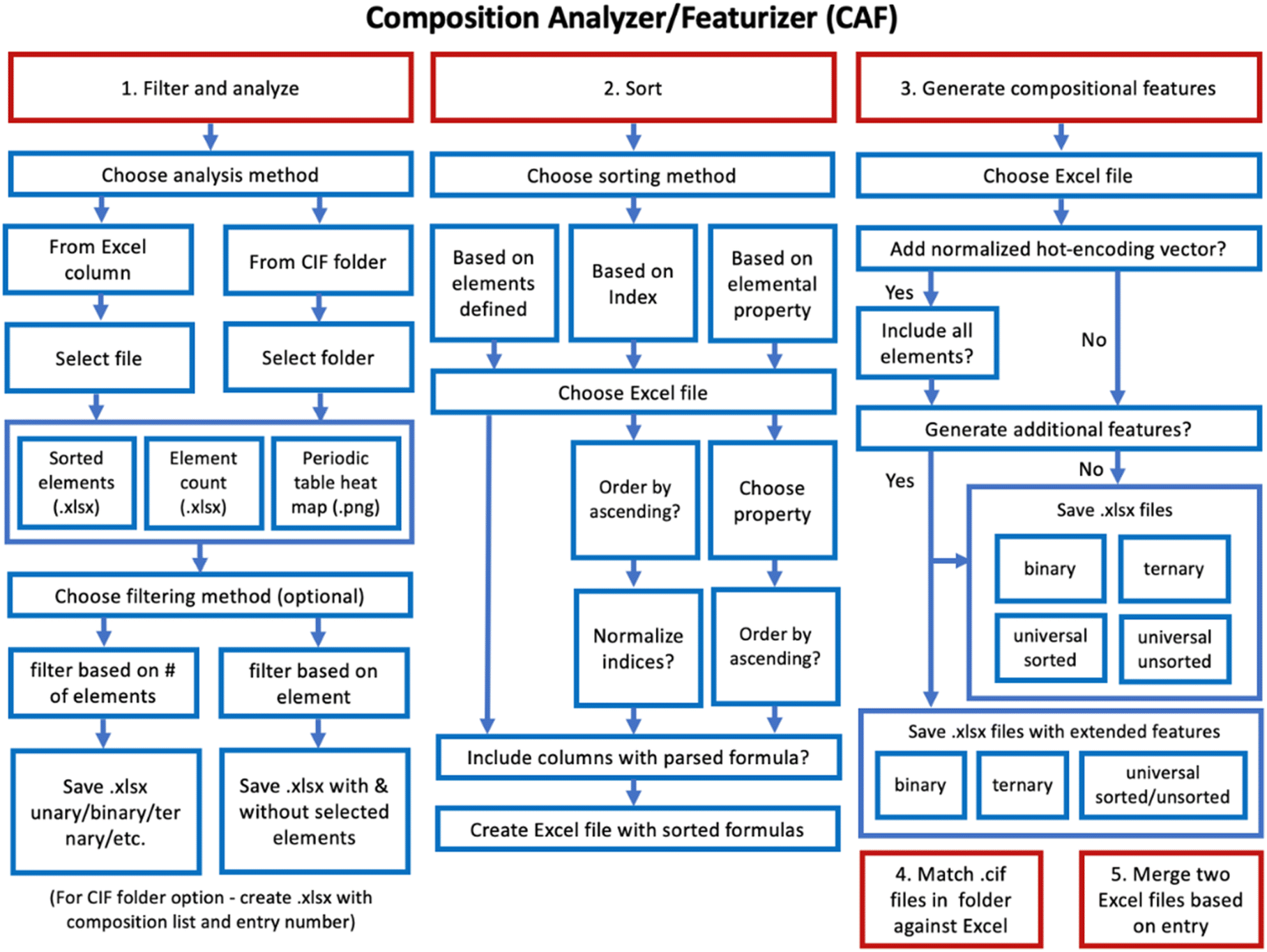Fig. 2 Options available in Composition Analyzer/Featurizer (CAF).

CAF is also designed for extensibility. The list of properties used for calculating features can be further enhanced by incorporating novel size or electronegativity scales defined by the user. For instance, the size scale is sensitive to the class of materials and the presence of other elements, making it advisable for users to calculate their own scale for effective modeling. For example, to define a new size scale, one could use the shortest homoatomic distance from CIF reports, divided by 2, to determine the CIF radius. We recommend generating the output with the mean value, standard deviation, and a histogram for visual inspection. The CIF radius scale can then be used as a property for feature definition, comparable to other metrics such as covalent radius, ionic radius, and others.

Structure featurization

We discuss a simple method of generating features from a composition, which can be augmented with information extracted from CIF files, including but not limited to the space group number and unit cell parameters. Additional features could be extracted from the database, which is specific to how the data there is structured (in our case, we used PCD⁷⁰). While these database-sourced features are not utilized in this study, they are further explored in the ESI Table S3.† Herein, we aim to extract additional information that is useful for describing the structure. The goal is to combine measurable descriptors with explainable models to help reveal intuitive relationships between the structure and properties. At the atomic level, the structural feature sets include information on coordination geometry, bond distances, and atomic environments. These structural features can be used either as standalone features or in combination with other compositional features to generate high-accuracy models, as demonstrated in this study.

Proposed here is the Structure Analyzer Featurizer (SAF) available at https://github.com/bobleesj/structure-analyzer-featurizer or https://github.com/OliynykLab/. At the time of writing, SAF currently supports binary and ternary compounds, generating 94 numerical features and 134 features for ternary with the goal to support quaternary and beyond for future studies. The complete lists of features are available in the GitHub repository and the ESI Tables S4–S6, with Table S4† providing comments that allow users to utilize extracted data not only for ML modeling but also for structure analysis. INT_* features are calculated from interatomic distance analysis, WYC_* features are based on Wyckoff symbol/multiplicity, ENV_* features are derived from atomic environment data, and CN_* features are also calculated from atomic environment data. Fig. 3 illustrates the process of procuring a single set of numerical features extracted from structural, compositional, and raw data as an input data source for ML models. Parts of the SAF code have been used to determine coordination geometry using various methods.⁷¹ Furthermore, although not implemented in this study, the features can be used for feature relationship analysis (e.g., SISSO) to reveal the relationships between the measured structural features and properties.⁷²

Fig. 3 Process for combining compositional and structural features with raw data.

SAF supports .cif files from databases such as PCD, ICSD, COD, and Materials Studio. PCD provides detailed structural descriptions, including editor-entered crystal structure prototypes and fully standardized crystal structure data. Similarly, we have ensured that our code is compatible with the ICSD database,⁷³ where most structures also have assigned structure types, which facilitates searches for specific structure classes. We recommend standardizing CIFs through trusted crystallographic software which writes CIFs in the correct format. Large CIF repositories do not guarantee consistency in CIF formatting, and even with large online databases, there could be cases when, for example, atomic label and atomic type are reversed, which might cause errors in file processing. Furthermore, CIFs, even from reputable databases, require some editing, due to typographic error or missing entries which prevents them from being parsed. Extracting data from databases might seem to be a straightforward process, but preparing the files for processing tends to require some adjustments. For instance, parsing errors might arise in cases where CIF info loops have blanks reported with some information missing. These could be as simple as the title of publication missing or author's affiliation, but these problems can affect file parsing. In materials science, especially where experimental data are scarce, it is crucial to ensure that all reports are included, and errors are automatically corrected. Another common CIF problem is inconsistent site labels, especially the numbering of labels or problematic labels in the case of atomic mixing, where the same site could be labeled differently, causing confusion and inconsistent results during a high-throughput CIF processing. Therefore, to filter ill-formatted CIF files, we have also developed a standalone and user-interactive Python application called CIF Cleaner available at https://github.com/bobleesj/cif-cleaner or https://github.com/OliynykLab/ (Fig. 4).

Fig. 4 User prompt options in CIF Cleaner code.

Data mining

To test featurizers and demonstrate our recent data processing developments, we selected the simplest 1 : 1 equiatomic compound cases, similar to the study done a decade ago,⁷⁴ but with a more challenging subset – intermetallics. (Compositionally unrestricted data for common structure types often could be easily segregated with self-reiterated parameters such as electronegativity.) The selected intermetallic data are provided in Table 2. The CIFs in this work were extracted from 2023/2024 versions of Pearson's Crystal Database (PCD).⁷⁰ In this study, we limited the dataset to the elements we use in our intermetallic research, provided in Fig. 5.

Table 2 The most common structure types for intermetallic 1 : 1 structures (at least 15 representatives)

Structure type	Search result	CIFs needed editing	Under ambient conditions
TlI	411	10	401
FeB	279	1	197
NaCl	243	1	236
FeSi	190	1	164
CsCl	188	4	138
ZnS	89	3	89
FeAs	86	1	79
NiAs	85	1	83
CuAu	47	3	41
Cu	141	1	104
Mg	32	0	29
W	15	0	0

---

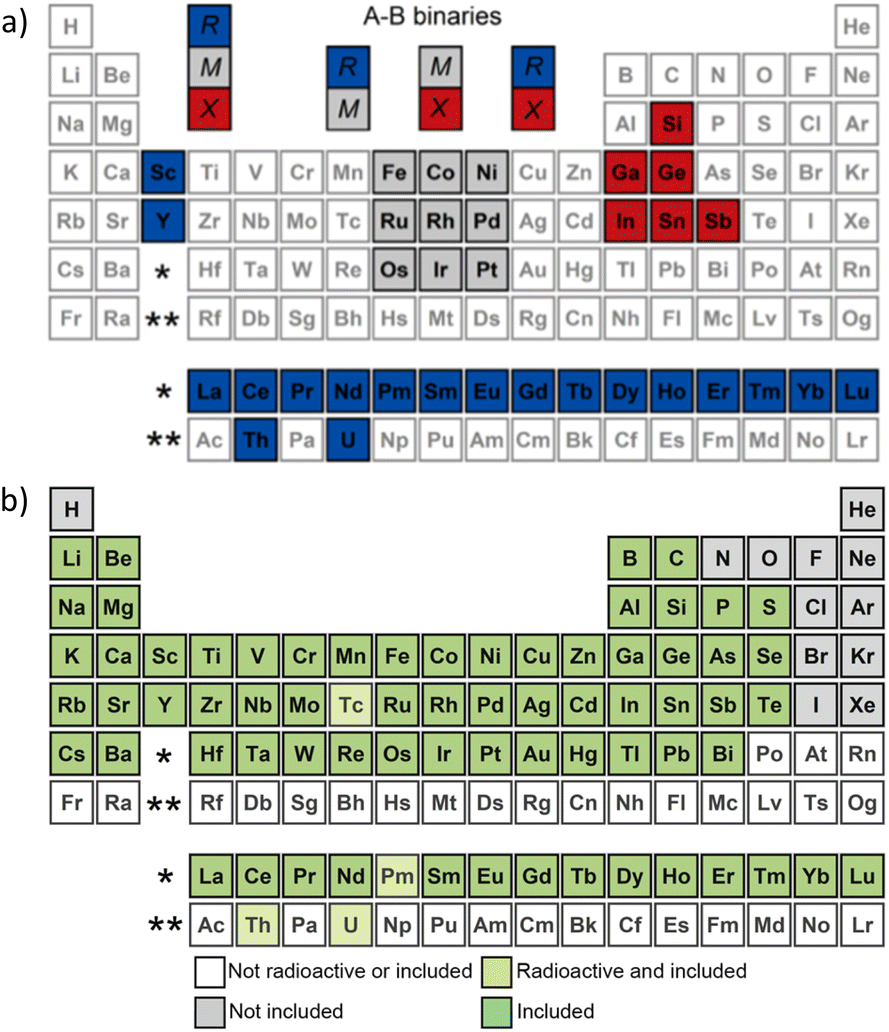Fig. 5 (a) Elements used in the current study to illustrate the application of Structure Analyzer Featurizer (SAF) and (b) all solid elements included in Composition Analyzer Featurizer (CAF).

Results and discussion

To compare the featurizers and test how the combination of compositional and structural features can influence the output, we prepared features using CBFV-embedded JARVIS, MAGPIE, mat2vec, and Oliynyk (OLED) featurizers and two sets of features prepared using the featurizers described in this work: Composition Analyzer Featurizer (CAF) and Structure Analyzer Featurizer (SAF). Although we focus our study on intermetallics, SAF and CAF, alongside the OLED dataset, have already been successfully applied to other problems, such as chalcogenides and thermoelectric materials.^75,76 The number of features that were generated is available in Table 3. In the cases where feature calculation resulted in infinity (Inf) or not a number value (NaN), these columns had to be ignored for the purpose of ML model training. These cases occur with generic featurizers quite commonly, given that division by zero occurs when a set of standard mathematical operations is looped through the list of element properties. One could replace these Inf and NaN with the best guess value; however, it is advised not to do that for preserving data in its original state. With our newest developments, CAF and SAF, we made sure to avoid calculations that result in problems, for example, by never dividing any property by the number of electrons at certain shells, which might result in the division by zero. For each feature case study, we employed three very common ML methods: PLS-DA, SVM, and XGBoost. The support vector machine (SVM) model produces similar results in terms of model statistics and time to train compared to XGBoost. In the current dataset, neither of the featurizers had issues with providing features sufficient to train and cross validate SVM models with the best model statistics (Table 3). Along with our feature sets, mat2vec also had marginally higher precision and recall compared to other datasets. As expected, we observed the ideal predictions with more expensive (SVM) models, which already showed effectiveness in solving crystallographic problems previously.^65,77 Our goal in this study is not attaining the best model statistics. The primary purpose of the study is to test how different sets of features perform with simpler methods (partial least squares discriminant analysis, PLS-DA) and to assess the visual clustering achieved through dimensionality reduction (latent values, LV, and individual feature contribution), similar to structure map approaches (Fig. 6). The performance of the models on each dataset is available at: https://github.com/bobleesj/SAF-CAF-performance. The estimated cost value in Table 3 is based on the time it takes to run all models (PLS-DA, SVM, and XGBoost) on a single core. For PLS-DA and SVM, we used stratified K-fold cross-validation with 10 splits, with data shuffling and random states provided in the source code. No further hyperparameter tuning was conducted. For PLS-DA plotting, the number of components was determined based on the best accuracy achieved with between 2 and 10 components.

Table 3 PLS-DA, SVM, and XGBoost model statistics based on various feature sets

	Features	PLS-DA				SVM				XGBoost				Cost
	Generated	Precision	Recall	F1-score	Accuracy	Precision	Recall	F1-score	Accuracy	Precision	Recall	F1-score	Accuracy
JARVIS	3066	0.372	0.366	0.330	0.391	0.979	0.965	0.977	0.972	0.989	0.985	0.987	0.989	23.7
MAGPIE	154	0.369	0.364	0.328	0.404	0.965	0.956	0.960	0.967	0.988	0.983	0.985	0.986	0.8
mat2vec	1400	0.611	0.658	0.582	0.609	0.990	0.985	0.987	0.989	0.981	0.978	0.979	0.983	9.3
OLED	308	0.449	0.448	0.399	0.457	0.974	0.955	0.963	0.973	0.987	0.984	0.985	0.987	1.4
CAF	133	0.419	0.384	0.363	0.404	0.967	0.950	0.957	0.959	0.988	0.984	0.986	0.987	1.03
SAF	94	0.526	0.567	0.511	0.603	0.993	0.989	0.991	0.990	0.997	0.993	0.995	0.994	0.6
CAF + SAF	227	0.569	0.589	0.533	0.579	0.994	0.987	0.991	0.993	0.997	0.996	0.996	0.996	1

---

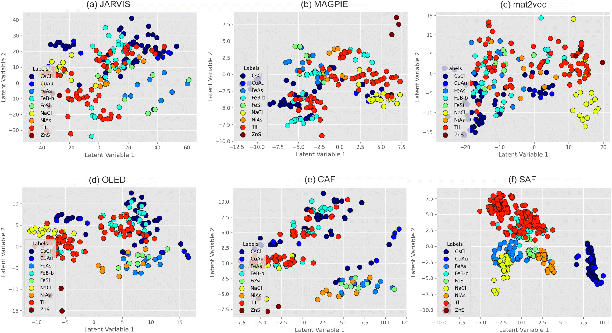Fig. 6 PLS-DA latent value plot using the first two latent value dimensions: (a) JARVIS, (b) MAGPIE, (c) mat2vec, (d) OLED (all sets of features were generated with CBFV), and our developments – (e) CAF and (f) SAF.

Among the featurizers used via CBFV (Fig. 6a–d), none demonstrate a clear class clustering in two dimensions, except for NaCl structures (yellow circles), especially with mat2vec. Clustering with CAF (Fig. 6e) also is not better than other composition-based featurizers, which is not surprising, given that it is based on the OLED set of properties for feature generation. The location of some datapoints with extreme values of LV1 and LV2 might indicate decreased confidence in their prediction as they are approaching the limits of the compositional space. JARVIS had precious metal silicides at the edge of the model confidence, which is typical for underrepresented cases such as OsSi (FeSi-type), IrSi (FeAs-type), and RhSi (in both FeAs- and CsCl-types). MAGPIE had some issues with classifying rare cases when the compounds are formed with two p-block elements, such as GaSb (ZnS-type), InSb (ZnS-type), and SnSb (ZnS- and NaCl-type). This is not surprising as most of the datasets consisted of transition metal-containing phases, and compounds with only main block elements are rare. Similar issues, and actually the same compounds, were problematic on the PLS-DA plot from the model based on OLED. One of the limitations of composition-based featurizers is their inability to handle polymorph cases, where one stoichiometry can form multiple structures, like it was in the cases described above (SnSb and RhSi).

CAF was developed with the output data consistency in mind and with a principle that treats differently integral values (measured exactly) and property values (measured over the range of values) to avoid Inf or NaN values in cells. CAF, SAF (Fig. 6e and f), and SAF + CAF (Fig. 7) models in PLS-DA plotted with reduced dimensions to two LV dimensions are shown to be complementary to each other. While CAF had NaCl points mixed with FeB and TlI and SAF had difficulties in segregating NaCl with FeAs, the combination of SAF + CAF (Fig. 7) resolved individual CAF and SAF issues completely. Some structure types have a wide composition range which results in partial success of structure segregation. For instance, the segregation of the TlI-type dataset depends on the element present in the TlI structure. The Fe-family member representative of the TlI class could not be efficiently separated from the rest of the structures; however, the rare-earth element TlI representatives are well separated with mat2vec (Fig. 6c, TlI points at LV1 = 8–15), SAF (Fig. 6f, TlI points at LV1 = −5.0 to −1.8 and LV2 = 2.5–8.0), and SAF + CAF (Fig. 7, TlI points at LV2 = −3 to −7). SAF analyzes geometry and is agnostic to the composition of the samples, resulting in clear clustering of the structures, besides a large cluster that has mixed TlI/FeB, and FeSi/FeAs/NiAs types in one. This clustering happens because of similar coordination geometry within the cluster but distinctly different from the rest of the structures. Traditionally, like in all previous plots, ZnS-type is at the edge of the confidence with extreme LV1 and LV2 values. Combination of CAF and SAF results in the solution to the large unseparated blocks mentioned above, with only two structure types overlapping (TlI and FeB), as shown in Fig. 7. None of the featurizers provided data to successfully separate these two structure types, but to be fair, mat2vec was the closest to separation compared to the rest of the featurizers.

Fig. 7 SAF + CAF PLS-DA plot.

Indirect problem solving with a crystal structure classification model

In chemistry, often ML models are created for a specific task and could not be applied to similar yet different datasets without loss of accuracy/precision/recall. Here, we tested the cases when a more specific structure classification problem was solved, and the solution was applied (including the dataset and features) to solve a more general problem. Next, we tested the extrapolation of machine learning models, when the model was built on a similar AB dataset, applied on a different AB dataset, which is too different to be considered as validation/test. As shown in Fig. 8a, the SAF + CAF model from our study is plotted with a structure type y-vector (9 classes), but the color-coded output is based on crystallographic compound classes (7 classes), where some structures are structurally similar and often grouped together. For example, TlI and FeB, which are both distorted variations of NaCl, require advanced tools to be separated with materials informatics.⁷⁸ These two structure types were segregated successfully with SVM and XGBoost, but no separation was observed with PLS-DA (Fig. 6). In the current case (Fig. 8a), the indirect learning of crystallographic compound classes (7 classes) through structure type classification (9 classes) is visually apparent and performed statistically even better than direct learning (Fig. 7), specifically because of the structural similarities of these structure types. On the other hand, another problem such as centrosymmetric/noncentrosymmetric classification (two classes), Fig. 8b, remains unsolved, which suggests a more complex phenomenon behind this classification, or the need for more specific features to approach this problem. In other cases, we applied our new expanded dataset to the model with a similar AB classification. Almost a decade ago, we tackled AB binary equiatomic classification for the first time, with experimental validation.³ A small dataset (yet, significantly larger than structure mapping approach used prior to that work)⁶⁹ was used, which resulted in a decent separation of structure types. It is important to note that the structure types used in that study differ from the ones used in the current study. No matter if the full feature set (56) or feature-selected set (33) was used, separation of the classes was not significantly different from any other composition featurizer. This is consistent with our expectations; none of the structure types were segregated within the LV space (Fig. 8c). Testing models for indirect problem solving or extrapolation helps us better understand the limitation of the models and apply them accordingly.

Fig. 8 Indirect learning with our model to solve problems of (a) compound class and (b) noncentrosymmetric phase prediction and (c) testing set of features from another AB classification model.

Explainability of the models

Explainable machine learning determines each feature's contribution to the output and the correlation between features, transforming a black-box model into a glass-box model, ultimately generating new knowledge. Let us look at how explainability has been used recently. In a recent study, post-hoc model interpretability methods such as BreakDown (BD) and SHapley Additive exPlanations (SHAP) were employed after building an ensemble of support vector machines used for phase classification of multi-principal element alloys.⁷⁹ The training data consisted of 1821 instances, each with 12 features such as mean melting point, mean enthalpy of formation, and mixing entropy. For BCC structure types, both BD and SHAP methods identified the mean melting temperature and maximum atomic weight difference as dominant variables. In another study, three gradient boosting methods, histogram gradient boosting (HGB), extreme gradient boosting (XGB), and gradient boosting (GB), were used to predict the adhesion strength of synthesized fibrillar dry adhesives, each characterized by 7 features such as contact area and pull-off force.⁸⁰ For each model, three explainable machine learning techniques (SHAP, LIME, and DALEX) provided both local and global contributions of each feature. The study demonstrates that explainable machine learning is a viable approach for limited datasets and limited number of features in experimental settings. Similar to our study, in the materials science discipline, SVM and XGBoost methods are common, as they result in excellent quality models, and explainability could either be achieved with post-hoc methods or be inherent to the model, like in the case with XGBoost.

Aiming for explainability in models, especially with structural descriptors, reveals correlations that advance chemical knowledge. For instance, it helps to develop new size or electronegativity scales for a specific subclass of compounds or analyze polyhedra through the lens of electron configurations and orbital hybridization theory. Structural features play an important role in the overall prediction of property schema in various situations. For instance, in a study analyzing ligand affinities, the authors ranked the features with three different methods, namely RF, Permutation Importance, and AdaBoost, which consistently placed PEOE_VSA2 and NumHAcceptors as the two highest-ranked features.⁸¹ These features are two-dimensional topological and topochemical properties that have versatile uses. However, the authors specifically needed them to provide valuable information about the molecular surface and its potential interactions with binding species. NumHAcceptors is self-explanatory, while PEOE_VSA calculates the atomic contributions to the van der Waals surface area using partial total charges and molar refractivity. In another paper predicting band gap for materials,⁸² the authors analyzed the respective features by using two different ranking criteria, one based on Pearson correlation between each of the fifteen features and the target variable and the other based on the weights obtained from Lasso regularization (weights of the Lasso coefficient). They were able to reduce the original set of fifteen features to seven with no loss of information. Another work had a similar schema using both a low number of descriptors (nine in total, a combination of elemental and structurally based) and found only one of those structural descriptors (octahedral factor) in the top five descriptor ranking.⁸³ They ranked these descriptors using recursive feature elimination, which selects features by recursively removing those which exhibit the smallest weight assigned by an extra tree classifier. Structural features were also used for bulk and shear modulus prediction (proxy properties for hardness),⁷⁷ where they were among the most important features after iterative feature selection. As we can see, structural features are used in building explainable models and could be easily identified in datasets with a small number of features. This allows detailed feature correlation analysis and straightforward construction of the decision trees, which are regarded as the most visual representation of model explainability.

In the current study, we deal with a larger set of features (a few hundred), which requires dimensionality reduction, while preserving the information on each feature importance. We believe that even simple methods like PLS-DA might be effective in solving crystallographic structure classification problems. And with an effective set of features (SAF + CAF), it could identify the same important features as more expensive (XGBoost) methods, providing us the explainability in an affordable way. While PLS-DA (as well as PCA) methods allow us to explore the LV (or PC) space and extract the weights of the original features that contribute to the axes, it is important to keep in mind that for these methods the combination of features matter more so than the individual features. In recent years, explainability has become an important topic as the age of the black box methods is over, and users want to gain insight rather than just getting results with excellent modelling statistics. (Often, for experimentalists, explainability that results in new chemical knowledge and eventually translates into novel material discovery is more important than high model accuracy statistics.) There are a few methods that improve the explainability/interpretability of the models, and here we summarize the top ten XGBoost scores for each feature set that was used in our test study (Fig. 9).^7,84,85

Fig. 9 XGBoost highest performing features from the models using various featurizers.

Labeling features is the first step to explainability, and despite being on a par with our featurizers in terms of model statistics, mat2vec fails to provide appropriate and scientifically meaningful labels for their features (Fig. 9c). In the top 10 features with the highest gain according to XGBoost, JARVIS identifies the mass, volume, and electron properties (ionization energy, electron affinity, etc.) to be the most important. MAGPIE identifies periodicity and systematization information (Mendeleev number, group number, and space group number), electron properties, and physical properties among the most important features. OLED shows a great balance of features in the top gain list, which consists of the periodic table information (group number), various size scales (metallic and Miracle radii), various electronegativity scales (Gordy and Pauling), and electron count approaches (metallic valence and valence electron count), along with the physical properties of different origins (polarizability, ionization energy, and specific heat). We continued the approach behind OLED featurization in our CAF development; therefore, CAF top features also demonstrate the excellent balance of features: periodic (group number and Mendeleev number), size (radii difference, average radius, and Pauling radius), Pauling electronegativity, and physical properties (bulk modulus, ionization energy, and melting point). It is important to mention that the user-introduced features such as the CIF radius scale introduced in this work and element preprocessing play a crucial role, since 8 out of 10 top features had a specific A/B element sorting tag. The CAF feature set is the closest to the classical structure map works by Villars and Pettifor.^64,69 SAF produces structural features, which are unique to other featurizers. The features are related to the coordination environment, interatomic distances, and distortions of polyhedra. Interestingly, the combined SAF + CAF (Fig. 9g) results in the most effective model, and the gain scores of the top two features overlap with the top two features from SAF (Fig. 9f) and CAF (Fig. 9e) separately, which is a great indication of the balance. While the top 10 features of SAF + CAF are dominated by the structural origin, as we will show next, PLS-DA LV contribution scores solve this issue, and compositional features become on a par with the structural features.

PLS-DA is an affordable method for analysis and modeling of large volumes of data. With a combination of a properly constructed feature vector, it becomes an effective method to increase the explainability. Ultimately, PLS-DA application in solid state chemistry originates from structural maps that were traditionally used in crystal structure classifications. While model statistics of PLS-DA are not comparable to SVM and XGBoost methods (Table 3), PLS-DA model statistics (which deviate more in the PLS-DA method) can provide an indication of a suitable feature set, when more advanced methods produce quite comparable results indifferent to the feature set. Another application of the PLS-DA method could be feature analysis for explainability. The first indication is variance percent in latent value vectors (LVs). With modern computational power, we have a privilege of utilizing any number of LVs we want, and the cumulative variance increases with more LVs. Eventually, the accuracy converges at certain LV levels, but the most effective number of LVs is usually low, with the first 3 LVs being the most helpful as it allows one to visualize data in plots, essentially creating structure maps. In our comparison, we looked at the two most accurate PLS-DA models, mat2vec and our development, SAF + CAF (Table 4). The cumulative variance of SAF + CAF is significantly higher than that of mat2vec, meaning that our features are used more effectively. While the first two LVs are dominated by SAF features, the CAF features are also present, especially in the third LV. In bold, we have highlighted the features that were listed in the top 10 gain features by the XGBoost model. In the case of mat2vec, only one feature had an overlap, while half of the features found to be helpful with XGBoost were also found in the first three LVs with the PLS-DA method. This is significant considering the relative cost of the methods and highlights how effective features from SAF and CAF are.

Table 4 Comparison of the top contributing features to the first 3 LVs of the best performing PLS-DA models

	mat2vec		SAF + CAF
	Variance	Top contributors	Variance	Top contributors
LV1	11.50%	max_53	15.26%	CN_MIN_packing_efficiency
		min_74		CN_AVG_packing_efficiency
		mode_74		CN_MAX_packing_efficiency
		min_178		WYK_A_lowest_wyckoff
		mode_178		WYK_B_lowest_wyckoff
		sum_46		WYK_A_multiplicity_total
		sum_84		WYK_B_multiplicity_total
		sum_129		CN_MIN_B_atom_count bulk_modulus_avg
		avg_46		ENV_B_shortest_tol_dist_count
		avg_84
LV2	2.82%	dev_193	11.82%	INT_UNI_refined_packing_efficiency
		range_193		ENV_B_count_at_A_shortest_dist
		min_23		ENV_B_avg_count_at_A_shortest_dist
		mode_23		INT_Asize_ref
		max_193		CN_AVG_central_atom_to_center_of_mass_dist
		dev_194		CN_MAX_central_atom_to_center_of_mass_dist
		range_194		CN_MIN_central_atom_to_center_of_mass_dist
		dev_91		ENV_A_shortest_dist_count
		range_91		ENV_A_avg_shortest_dist_count
		dev_195		CN_AVG_packing_efficiency
LV3	4.79%	max_75	4.56%	specific_heat_A–B
		dev_129		specific_heat_B
		range_129		ENV_A_count_at_A_shortest_dist
		min_40		ENV_A_avg_count_at_A_shortest_dist period_B
		min_50		CN_MAX_B_atom_count specific_heat_A/B
		mode_40		Z_eff_B ratio_closest_min
		mode_50		density_A/B
		sum_40
		avg_40
		dev_191

---

Conclusions

Combination of various features from different sources and generated using various approaches is important. We provided a tool that besides generating our features also allows users to integrate features from other sources by combining data matrices. The most important role in explainability is preprocessing and tailoring dataset and features to a specific problem, such as organizing a structure/formula in a meaningful way and introducing novel features, such as CIF radius. We built open-source command-line-based Python programs known as Composition Analyzer Featurizer (CAF) and Structure Analyzer Featurizer (SAF), which work with all elements that exist in their solid form under ambient conditions. These featurizers produce well-balanced and superior quality features readily available to be applied in machine learning models or used for classical structural map plotting. CAF generates numerical compositional features from a list of formulae provided in an Excel file, while SAF extracts numerical structural features from a .cif file by generating a supercell. To expedite the current state of machine learning and make sure it is more accessible, we kept in mind that most users may not have a computational background and therefore included that subjective experience when developing our software. We also looked at various solid state applicable featurizers already in use to provide a benchmark for ourselves and the reader. To emphasize the needs of the user, we ensured our software checked every box and included various options within filtering, sorting, checking, and providing multiple visualizations for the user to have the smoothest experience possible while maintaining scientific knowledge. For validation, 133 features from CAF and 94 features from SAF were either combined or used separately to classify structures in equiatomic AB intermetallics. From the explainable model, a novel size scale CIF radius, various structural features, such as distortion of polyhedra, and data preprocessing were found to be important. The performance, measured in terms of precision, recall, F1-score, and accuracy, was comparable to and surpassed those generated using features from JARVIS, MAGPIE, mat2vec, and OLED in PLS-DA and SVM. The combination of CAF and SAF showed promising results in addressing these challenges, suggesting potential for enhanced performance in crystallographic problem-solving tasks compared to other featurizers. Further research should focus on optimizing the integration of CAF and SAF, to fully realize their potential in improving the performance and efficiency in these crystallographic systems.

Data availability

Composition Analyzer Featurizer (CAF) software: https://github.com/bobleesj/composition-analyzer-featurizer or https://github.com/OliynykLab/. Structure Analyzer Featurizer (SAF) software: https://github.com/bobleesj/structure-analyzer-featurizer or https://github.com/OliynykLab/. CIF Cleaner software: https://github.com/bobleesj/cif-cleaner or https://github.com/OliynykLab/. Structure Analyzer Featurizer (SAF) and Composition Analyzer Featurizer (CAF) performance: https://github.com/bobleesj/SAF-CAF-performance.

Author contributions

Anton Oliynyk: data curation, formal analysis, visualization, writing – original draft, writing – review & editing, software, supervision. Lee Sangjoon: software, data curation, formal analysis, writing – review & editing. Emil Jaffal: software, data curation, formal analysis, writing – review & editing. Nikhil Barua Kumar: software. Holger Kleinke: editing. Danila Shiryaev: software. Alex Vtorov: software.

Conflicts of interest

All authors declare that there are no conflicts of interest.

Acknowledgements

AOO is thankful for the startup funding support provided by Hunter College CUNY.

Notes and references

1. F. Oviedo, J. L. Ferres, T. Buonassisi and K. T. Butler, Acc. Mater. Res., 2022, 3, 597–607.
2. J. Dean, M. Scheffler, T. A. R. Purcell, S. V. Barabash, R. J. Dean, M. Scheffler, T. A. R. Purcell, S. V. Barabash, R. Bhowmik and T. Bazhirov, J. Mater. Res., 2023, 38, 4477–4496.
3. A. O. Oliynyk, L. A. Adutwum, J. J. Harynuk and A. Mar, Chem. Mater., 2016, 28, 6672–6681.
4. B. Selvaratnam, A. O. Oliynyk and A. Mar, Inorg. Chem., 2023, 62, 10865–10875.
5. S. M. Lundberg and S.-I. Lee, Advances in Neural Information Processing Systems, 2017.
6. T. Chen and C. Guestrin, Presented in part at the Proceedings of the 22nd ACM SIGKDD International Conference on Knowledge Discovery and Data Mining, San Francisco, California, USA, 2016.
7. S. Lipovetsky and M. Conklin, Applied Stochastic Models in Business and Industry, 2001, vol. 17, pp. 319–330.
8. A. A. K. Farizhandi, O. Betancourt and M. Mamivand, Sci. Rep., 2022, 12, 4552.
9. A. Y.-T. Wang, S. K. Kauwe, R. J. Murdock and T. D. Sparks, npj Comput. Mater., 2021, 7, 77.
10. R. Woods-Robinson, D. Broberg, A. Faghaninia, A. Jain, S. S. Dwaraknath and K. A. Persson, Chem. Mater., 2018, 30, 8375–8389.
11. S. Kauwe, A. Wang and A. Falkowski: CBFV: Tool for quickly creating a composition-based feature vector, 2021, https://pypi.org/project/CBFV/.
12. L. Ward, A. Dunn, A. Faghaninia, N. E. R. Zimmermann, S. Bajaj, Q. Wang, J. Montoya, J. Chen, K. Bystrom, M. Dylla, K. Chard, M. Asta, K. A. Persson, G. J. Snyder, I. Foster and A. Jain, Comput. Mater. Sci., 2018, 152, 60–69.
13. A. Jain, S. P. Ong, G. Hautier, W. Chen, W. D. Richards, S. Dacek, S. Cholia, D. Gunter, D. Skinner, G. Ceder and K. A. Persson, APL Mater., 2013, 1, 011002.
14. Chemical & Materials Development Platform, accessed February 2024, https://citrine.io/.
15. B. Blaiszik, K. Chard, J. Pruyne, R. Ananthakrishnan, S. Tuecke and I. Foster, JOM, 2016, 68, 2045–2052.
16. Materials Platform for Data Science, accessed February 2024, https://mpds.io/#start.
17. L. Ward, A. Agrawal, A. Choudhary and C. Wolverton, npj Comput. Mater., 2016, 2, 16028.
18. S. Kumar, S. Dutta, R. Jaafreh, N. Singh, A. Sharan, K. Hamad and D. H. Yoon, Mater. Lett., 2023, 353, 135311.
19. V. Stanev, C. Oses, A. G. Kusne, E. Rodriguez, J. Paglione, S. Curtarolo and I. Takeuchi, npj Comput. Mater., 2018, 4, 29.
20. F. Ren, L. Ward, T. Williams, K. J. Laws, C. Wolverton, J. Hattrick-Simpers and A. Mehta, Sci. Adv., 2018, 4, eaaq1566.
21. K. Choudhary, K. F. Garrity, A. C. E. Reid, B. DeCost, A. J. Biacchi, A. R. Hight Walker, Z. Trautt, J. Hattrick-Simpers, A. G. Kusne, A. Centrone, A. Davydov, J. Jiang, R. Pachter, G. Cheon, E. Reed, A. Agrawal, X. Qian, V. Sharma, H. Zhuang, S. V. Kalinin, B. G. Sumpter, G. Pilania, P. Acar, S. Mandal, K. Haule, D. Vanderbilt, K. Rabe and F. Tavazza, npj Comput. Mater., 2020, 6, 173.
22. K. Choudhary, I. Kalish, R. Beams and F. Tavazza, Sci. Rep., 2017, 7, 5179.
23. S. Im, S.-L. Shang, N. D. Smith, A. M. Krajewski, T. Lichtenstein, H. Sun, B. J. Bocklund, Z.-K. Liu and H. Kim, Acta Mater., 2022, 223, 117448.
24. P. Henkel, J. Li, G. K. Grandhi, P. Vivo and P. Rinke, Chem. Mater., 2023, 35, 7761–7769.
25. Q. Zhou, P. Tang, S. Liu, J. Pan, Q. Yan and S.-C. Zhang, Proc. Natl. Acad. Sci. U. S. A., 2018, 115, E6411–E6417.
26. E. R. Antoniuk, G. Cheon, G. Wang, D. Bernstein, W. Cai and E. J. Reed, npj Comput. Mater., 2023, 9, 155.
27. Y. Zhao, Y. Cui, Z. Xiong, J. Jin, Z. Liu, R. Dong and J. Hu, ACS Omega, 2020, 5, 3596–3606.
28. Z. Xiong, Y. Cui, Z. Liu, Y. Zhao, M. Hu and J. Hu, Comput. Mater. Sci., 2020, 171, 109203.
29. V. Tshitoyan, J. Dagdelen, L. Weston, A. Dunn, Z. Rong, O. Kononova, K. A. Persson, G. Ceder and A. Jain, Nature, 2019, 571, 95–98.
30. D. Ho, A. S. Shkolnik, N. J. Ferraro, B. A. Rizkin and R. L. Hartman, Comput. Chem. Eng., 2020, 141, 107026.
31. C. Thorne and S. Akhondi, arXiv, 2020, preprint, arXiv: 201012912, DOI: DOI:10.48550/arXiv.2010.12912.
32. D. Jha, L. Ward, A. Paul, W.-k. Liao, A. Choudhary, C. Wolverton and A. Agrawal, Sci. Rep., 2018, 8, 17593.
33. D. Jha, K. Choudhary, F. Tavazza, W.-k. Liao, A. Choudhary, C. Campbell and A. Agrawal, Nat. Commun., 2019, 10, 5316.
34. A. Vasylenko, J. Gamon, B. B. Duff, V. V. Gusev, L. M. Daniels, M. Zanella, J. F. Shin, P. M. Sharp, A. Morscher, R. Chen, A. R. Neale, L. J. Hardwick, J. B. Claridge, F. Blanc, M. W. Gaultois, M. S. Dyer and M. J. Rosseinsky, Nat. Commun., 2021, 12, 5561.
35. T. Xie and J. C. Grossman, Phys. Rev. Lett., 2018, 120, 145301.
36. C. W. Park and C. Wolverton, Phys. Rev. Mater., 2020, 4, 063801.
37. R. Wang, Y. Zhong, X. Dong, M. Du, H. Yuan, Y. Zou, X. Wang, Z. Lin and D. Xu, Inorg. Chem., 2023, 62, 4716–4726.
38. U. S. Vaitesswar, D. Bash, T. Huang, J. Recatala-Gomez, T. Deng, S.-W. Yang, X. Wang and K. Hippalgaonkar, Digital Discovery, 2024, 3, 210–220.
39. RDKit: Open-source cheminformatics, accessed February 2024, http://www.rdkit.org.
40. S. Hirte, O. Burk, A. Tahir, M. Schwab, B. Windshügel and J. Kirchmair, Cells, 2022, 11, 1253.
41. T. Doğan, E. Akhan Güzelcan, M. Baumann, A. Koyas, H. Atas, I. R. Baxendale, M. Martin and R. Cetin-Atalay, PLoS Comput. Biol., 2021, 17, e1009171.
42. H. Gao, T. J. Struble, C. W. Coley, Y. Wang, W. H. Green and K. F. Jensen, ACS Cent. Sci., 2018, 4, 1465–1476.
43. H. Moriwaki, Y.-S. Tian, N. Kawashita and T. Takagi, J. Cheminf., 2018, 10, 4.
44. D. N. Prada Gori, S. Ruatta, M. Fló, L. N. Alberca, C. L. Bellera, S. Park, J. Heo, H. Lee, K.-H. P. Park, O. Pritsch, D. Shum, M. A. Comini and A. Talevi, Front. Drug Discovery, 2023, 2, 1082065.
45. E. G. Tse, L. Aithani, M. Anderson, J. Cardoso-Silva, G. Cincilla, G. J. Conduit, M. Galushka, D. Guan, I. Hallyburton, B. W. J. Irwin, K. Kirk, A. M. Lehane, J. C. R. Lindblom, R. Lui, S. Matthews, J. McCulloch, A. Motion, H. L. Ng, M. Öeren, M. N. Robertson, V. Spadavecchio, V. A. Tatsis, W. P. van Hoorn, A. D. Wade, T. M. Whitehead, P. Willis and M. H. Todd, J. Med. Chem., 2021, 64, 16450–16463.
46. V. Saini, R. Kataria and S. Rajput, Artif. Intell. Chem., 2024, 2, 100032.
47. Z. Cao, R. Magar, Y. Wang and A. Barati Farimani, J. Am. Chem. Soc., 2023, 145, 2958–2967.
48. L. Himanen, M. O. J. Jäger, E. V. Morooka, F. Federici Canova, Y. S. Ranawat, D. Z. Gao, P. Rinke and A. S. Foster, Comput. Phys. Commun., 2020, 247, 106949.
49. F. Musil, A. Grisafi, A. P. Bartók, C. Ortner, G. Csányi and M. Ceriotti, Chem. Rev., 2021, 121, 9759–9815.
50. E. Gelžinytė, M. Öeren, M. D. Segall and G. Csányi, J. Chem. Theory Comput., 2024, 20, 164–177.
51. R. J. Bunting, F. Wodaczek, T. Torabi and B. Cheng, J. Am. Chem. Soc., 2023, 145, 14894–14902.
52. J. Lym, G. H. Gu, Y. Jung and D. G. Vlachos, J. Phys. Chem. C, 2019, 123, 18951–18959.
53. T. Mou, X. Han, H. Zhu and H. Xin, Curr. Opin. Chem. Eng., 2022, 36, 100825.
54. Z. C. C. Fu, Y. Wang and L. Zhang, SIAM International Conference on Data Mining (SDM), Houston, TX, April, 2024.
55. Y.-Y. Chen, M. Ross Kunz, X. He and R. Fushimi, Curr. Opin. Chem. Eng., 2022, 37, 100843.
56. S. Jodeh, Jordan J. Chem., 2008, 3, 281–292.
57. R. G. Barrows and J. B. Newkirk, Metallogr, 1972, 5, 515–541.
58. E. F. Kneller, J. Appl. Phys., 1964, 35, 2210–2211.
59. G. Viswanathan, A. O. Oliynyk, E. Antono, J. Ling, B. Meredig and J. Brgoch, Inorg. Chem., 2019, 58, 9004–9015.
60. L. Pauling, J. Am. Chem. Soc., 1932, 54, 3570–3582.
61. J. K. Nagle, J. Am. Chem. Soc., 1990, 112, 4741–4747.
62. R. S. Mulliken, J. Chem. Phys., 1934, 2, 782–793.
63. A. L. Allred and E. G. Rochow, J. Inorg. Nucl. Chem., 1958, 5, 264–268.
64. D. G. Pettifor, Solid State Commun., 1984, 51, 31–34.
65. A. S. Gzyl, A. O. Oliynyk, L. A. Adutwum and A. Mar, Inorg. Chem., 2019, 58, 9280–9289.
66. A. O. Oliynyk, L. A. Adutwum, B. W. Rudyk, H. Pisavadia, S. Lotfi, V. Hlukhyy, J. J. Harynuk, A. Mar and J. Brgoch, J. Am. Chem. Soc., 2017, 139, 17870–17881.
67. D. Mendeleev, Z. Chem., 1869, 12, 405–406.
68. L. S. Smith, D. K. Tappin and M. Aindow, Scr. Mater., 1996, 34, 227–234.
69. P. Villars, J. Less-Common Met., 1983, 92, 215–238.
70. P. Villars and K. Cenzual, Pearson's Crystal Data-Crystal Structure Database for Inorganic Compounds, ASM International, Materials Park, Ohio, USA, 2010.
71. Y. Tyvanchuk, V. Babizhetskyy, S. Baran, A. Szytuła, V. Smetana, S. Lee, A. O. Oliynyk and A.-V. Mudring, J. Alloys Compd., 2024, 976, 173241.
72. R. Ouyang, S. Curtarolo, E. Ahmetcik, M. Scheffler and L. M. Ghiringhelli, Phys. Rev. Mater., 2018, 2, 083802.
73. I. Levin, NIST Inorganic Crystal Structure Database (ICSD), 2015,  DOI:10.18434/M32147, https://data.nist.gov/od/id/mds2-2147.
74. F. Faber, A. Lindmaa, O. A. von Lilienfeld and R. Armiento, arXiv, 2015, preprint, arXiv: 150307406, DOI:  DOI:10.48550/arXiv.1503.07406.
75. N. K. Barua, S. Lee, A. O. Oliynyk and H. Kleinke, ACS Appl. Mater. Interfaces, 2024, 1661–1673.
76. S. Lee, C. Chen, G. Garcia and A. Oliynyk, Data Brief, 2024, 53, 110178.
77. A. Mansouri Tehrani, A. O. Oliynyk, M. Parry, Z. Rizvi, S. Couper, F. Lin, L. Miyagi, T. D. Sparks and J. Brgoch, J. Am. Chem. Soc., 2018, 140, 9844–9853.
78. V. Gvozdetskyi, B. Selvaratnam, A. O. Oliynyk and A. Mar, Chem. Mater., 2023, 35, 879–890.
79. K. Lee, M. V. Ayyasamy, Y. Ji and P. V. Balachandran, Sci. Rep., 2022, 12, 11591.
80. I. U. Ekanayake, S. Palitha, S. Gamage, D. P. P. Meddage, K. Wijesooriya and D. Mohotti, Mater. Today Commun., 2023, 36, 106545.
81. S. Chaube, S. Goverapet Srinivasan and B. Rai, Sci. Rep., 2020, 10, 14322.
82. F. Khmaissia, H. Frigui, M. Sunkara, J. Jasinski, A. M. Garcia, T. Pace and M. Menon, Comput. Mater. Sci., 2018, 147, 304–315.
83. A. Talapatra, B. P. Uberuaga, C. R. Stanek and G. Pilania, Commun. Mater., 2023, 4, 46.
84. A. Shrikumar, P. Greenside and A. Kundaje, arXiv, 2019, preprint, arXiv: 170402685, DOI:  DOI:10.48550/arXiv.1704.02685.
85. Y. Xu and Q. Qian, Eng. Appl. Artif. Intell., 2022, 116, 105442.

---

Footnotes

† Electronic supplementary information (ESI) available. See DOI: https://doi.org/10.1039/d4dd00332b

‡ These authors contributed equally to this work.

---