Scientific exploration with expert knowledge (SEEK) in autonomous scanning probe microscopy with active learning

Abstract

Microscopy plays a foundational role in materials science, biology, and nanotechnology, offering high-resolution imaging and detailed insights into properties at the nanoscale and atomic level. Microscopy automation via active machine learning approaches is a transformative advancement, offering increased efficiency, reproducibility, and the capability to perform complex experiments. Our previous work on autonomous experimentation with scanning probe microscopy (SPM) demonstrated an active learning framework using deep kernel learning (DKL) for structure–property relationship discovery. Here we extend this approach to a multi-stage decision process to incorporate prior knowledge and human interest into DKL-based workflows, we operationalize these workflows in SPM. By integrating expected rewards from structure libraries or spectroscopic features, we enhanced the exploration efficiency of autonomous microscopy, demonstrating more efficient and targeted exploration in autonomous microscopy. These methods can be seamlessly applied to other microscopy and imaging techniques. Furthermore, the concept can be adapted for general Bayesian optimization in material discovery across a broad range of autonomous experimental fields.

---

Introduction

Microscopy techniques are indispensable tools in materials science, biology, and nanotechnology, driving innovations by providing insights into the structural and functional characteristics of materials at the micro, nano-, and atomic scales. Techniques such as Atomic Force Microscopy (AFM) have revolutionized our ability to visualize and manipulate matter with nanoscale precision.¹ AFM not only offers high-resolution imaging by scanning a sharp probe over the sample surface for investigation of mechanical,^2,3 electrical,^4–6 and chemical properties^7,8 at the nanoscale, but also offers detailed insights into local dynamics by applying temporal excitation at nanoscale structures.^9–15

The automation of microscopy experiments can be expected to be one of the most transformative advancement in the field^16–25 vastly increasing the efficiency of data acquisition and use. Automated microscopy can offer comprehensive insights into material properties, systematically studying material behavior under a spectrum of conditions by adjusting experiment parameters such as scan size and excitation bias in an automatic manner.^26–28 These automated systems provide numerous benefits, including increased throughput, improved reproducibility, and the ability to perform experiments that would be impractical or impossible manually.

The rapid rise of machine learning (ML) applications in microscopy^29–36 has also significantly enhanced the field by assisting in instrument tuning,^37,38 data processing and analysis,^39–45 and acquisition.^46–50 In microscopy data analysis, ML can process vast amounts of data to uncover patterns and correlations that are not immediately apparent to human analysts,^51–57 accelerating the analysis process. In on-the-fly experiments, ML facilitates the development of autonomous experimentation systems by leveraging microscopy automation, ML algorithms, and workflow integration to perform experiments with minimal human intervention.^23,58,59 By integrating ML, researchers can design experiments, optimize imaging conditions, and even make decisions about subsequent measurements based on real-time data analysis.^47,50,60 This level of automation and intelligence is transforming microscopy into a more powerful and efficient tool, driving advancements in fields such as materials science, nanotechnology, and biology.

Generally, by now three levels of ML applications in microscopy can be defined. On the simplest level, ML is used as a part of data analysis after the experiment. These applications offer a broader toolbox of image and analysis methods compared to classical image analysis tools, but do not significantly change the nature of the microscopy experiment.^{33,38,61–66} The implementation of the ML image analysis methods as a part of the experiment offers real time segmentation and dimensionality reduction of data,^67–69 ultimately facilitating the representation of high dimensional and complex data to a human operator. This significantly increases requirements placed on the used ML algorithms, particularly towards out of distribution shifts.⁶⁷ However, real-time image analytics still requires human decision making. Finally, the third level of ML implementation is having ML agents directly controlling the instrument though suitable API or a software library. In this approach, the decision can be purely ML driven,^43,70,71 or the behavior of the ML agent including decision making policies and reward functions can be continuously tuned by a human operator, giving rise to human in the loop approach.^{19,33,34,61,72}

Previously we have implemented the autonomous experiment (AE) in scanning probe microscopy (SPM) for structure–property discovery using static and dynamic policies. In the former, the pretrained ML algorithms identify a priori known objects of interest and perform specific experiments using predefined policies. An example of this approach is to identify domain walls in ferroelectric samples and grain boundaries in hybrid perovskites,^12,46 enabling the discoveries of high responsive ferroelastic domain walls and insulating grain boundary junctions, respectively.

An alternative is the spectral discovery experiments, where an ML algorithm aims to discover which microstructures optimize certain spectral features. Unlike the static policy experiment where ML performs human-level semantic segmentation tasks, this is an example of beyond-human AE. We recently implemented an active learning framework using deep kernel learning (DKL)⁵⁰ that can uncover the relationship between image and spectroscopic data, namely the structure–property relationship. This approach has demonstrated broad applications in AFM,²² scanning tunneling microscopy,⁷³ and scanning electron transmission microscopy,^33,47 and can also be adapted for any other imaging and spectroscopy techniques. DKL enhances the capabilities of these systems by providing real-time data analysis and decision-making, enabling the identification of image patterns that are potentially interesting for spectroscopic investigation. In the process, DKL equally explores the entire region; however, in materials science, intriguing physics or functionality is often associated with specific structures or embedded in particular spectroscopic features. Instead of equally exploring the entire structure library and spectroscopic results, prior knowledge and expertise can be applied to refine the exploration space in DKL to enhance the discovery of intriguing functionality.

Both static and simple dynamic workflows have a number of limitations with respect to broad variability of surface responses and tunability of reward functions. Here, we report methods to incorporate prior knowledge and human interest into DKL-driven microscopy, engendering the transition from simple discovery loops to multi-stage decision making. We refer to this approach as Scientific Exploration with Expert Knowledge (SEEK). We demonstrate that prior knowledge and expected rewards can be integrated both from the structure library or the spectroscopic features for DKL exploration. When a constraint is applied to the structure, a machine learning method can analyze the acquired full structural image, identify the structure of interest based on human knowledge, and then form a structure library that includes only the structures of interest for DKL exploration. When a constraint is applied to the spectroscopic features, a second surrogate model predicts the target spectroscopic features, interacting with the acquisition function to determine the next measurement location. We implemented these approaches in both pre-acquired AFM model data and operating AFM experiment, revealing a more efficient exploration of autonomous microscopy.

Results and discussion

Traditional DKL-driven discovery

Fig. 1 and pseudo code 1 illustrate the process of a standard DKL-driven exploration, which begins with acquiring a 2D structural image, such as topography or piezoresponse force microscopy (PFM) images. From this structural image, we create image patches centered on individual pixels, which form a structure library representing the nanoscale spatial structure. Detailed properties at each pixel are measured via a spectroscopic mode, such as piezoresponse spectroscopy, force–displacement spectroscopy, current–voltage curves, etc. The acquired spectrum is analyzed by using a pre-defined scalarizer function to extract a physical descriptor for DKL training. At the beginning of a DKL-driven experiment, a few spectra are acquired at random or strategically selected locations. The DKL model is then trained using structure patches from these locations and corresponding physical descriptors from the measured spectra. The DKL model learns a probabilistic relationship between structure patches and physical descriptors, predicting the physical descriptor values for structure patches where spectra have not yet been measured. Utilizing DKL prediction and uncertainty for unmeasured pixels, an acquisition function determines the next structure patch (pixel) for spectroscopic measurement. After each new measurement, the DKL model is retrained with the updated training dataset, incorporating new structure patches and physical descriptors, thereby iterating the process. This iterative approach enhances the efficiency and accuracy of discovering structure–property relationships in high-dimensional datasets.

Fig. 1 Traditional DKL driven discovery. Image patches representing local structures are prepared on dense grid locations within an acquired full structure image. At the beginning, a few spectra can be measured at random locations, and all spectra are analyzed by using a scalarizer function to convert 1D spectra data to scalar physical descriptors. The corresponding image patches and descriptors at measured locations form a training dataset for DKL training, followed by DKL prediction at unmeasured locations. Then, an acquisition function derives the next spectrum measurement location and microscopy performs the next measurement, and the process is repeated until a certain criterion is achieved.

Pseudocode 1: traditional DKL
Input	Structural patch size ω; iterations N
Acquire a full structure image: I
Extract structural patches: X ← I, ω
	Structural patches are extracted from I on grid locations; ω as the patch size
Measure spectra Ss at seed patches Xs
	Seed patches can be selected randomly or by an expert
Extract physical descriptors: ys ← Ss
Prepare DKL training dataset: {Xtrain} ← Xs; {ytrain} ← ys
For n = 1, 2,…, N, do:
	Train DKL on {{Xtrain}, {ytrain}} and make prediction on properties of unmeasured patches
	Calculate the acquisition score: Acqn
	Measure spectra Sn at patch Xn ← argmax Acqn
	Extract physical descriptor: yn ← Sn, and update the training dataset: Xtrain ← Xn∪{Xtrain}; ytrain ← yn∪{ytrain}
Output:	• Measured structure patches and corresponding spectra, which demonstrate the property of interest or structure–property relationship
	• Estimation of properties for unmeasured structure patches
	• Trajectory of the learning process

Gated-DKL with a structure constraint

Pseudocode 2: gated-DKL with a structure constraint
Input:	Structural patch size ω; iterations N;
Acquire a full structure image: I
Prepare a binary classifier for the structures of interest: Imask
	The classifier can be prepared using the image segmentation method
Extract structural patches of interest: X ← I, Imask, ω
	Structural patches are extracted from I on masked locations Imask; ω as the patch size
Measure spectra Ss at seed patches Xs
	Seed patches can be selected randomly or by an expert
Extract physical descriptors: ys ← Ss
Prepare the DKL training dataset: {Xtrain} ← Xs; {ytrain} ← ys
For n = 1, 2, …, N, do:
	Train DKL on {{Xtrain}, {ytrain}} and make prediction on properties of unmeasured patches
	Calculate the acquisition score: Acqn
	Measure spectra Sn at patch Xn ← argmax Acqn
	Extract the physical descriptor: yn ← Sn, and update the training dataset: Xtrain ← Xn∪{Xtrain}; ytrain ← yn∪{ytrain}
Output:	• Structure patches or interest
	• Measured structure patches and corresponding spectra, which demonstrate the property of interest or structure–property relationship
	• Estimation of properties for unmeasured structure patches
	• Trajectory of the learning process

Typically, structure patches are prepared at uniform dense grid locations within a full structure image (as shown in Fig. 1). This approach allows the DKL framework to explore the entire region under study evenly, with spectroscopic measurement locations determined solely by the acquisition function. However, in materials research, properties of interest are often concentrated in specific areas, such as domain walls in ferroelectric materials or grain boundaries in photovoltaic perovskites. By focusing on structural patches related to these critical locations, we could potentially accelerate the discovery of relevant structure–property relationships. To leverage this prior knowledge, we propose a more targeted approach, as outlined in Fig. 2 and pseudocode 2. First, a binary classifier is prepared to identify the structures of interest within the full image. Using this classifier, structure patches are extracted only from locations corresponding to the structures of interest, resulting in a structure library that exclusively represents these regions. Consequently, the DKL exploration will be focused solely on these structures of interest, enhancing the efficiency of discovering structure–property relationships in these critical areas.

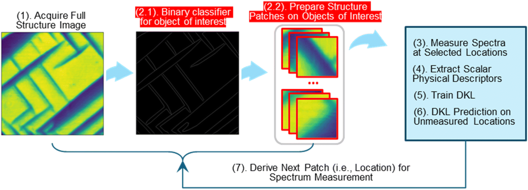Fig. 2 Structure-constrained DKL. Before preparing the structure patches, the structure of interest (e.g., ferroelastic domain walls) can be identified from the full structure image using a neural network or other methods (i.e. 2.1), and then the structure patches are only prepared on these identified locations to form a structure library (i.e. 2.2) only containing structures of interest for DKL exploration. As such, DKL-driven discovery will specifically focus on these structures of interest. In the workflow, the neural network (2.1) either serves as a binary classifier that defines objects as interesting/not interesting or ascribes an “interest score” to each patch that can be used to sample from when choosing the next object. This neural network can be trained, or the method can be defined prior to the experiment based on human interest and knowledge.

We first showcase the application of the structure-constrained DKL in a model dataset. This model dataset includes vertical band excitation piezoresponse spectroscopy (BEPS) data of a PbTiO₃ (PTO) thin film. This PTO material has been explored via various machine learning empowered automated and autonomous microscopy previously,^22,46,50,74 suggesting that it is a good model system for developing ML in materials science. Fig. 3a shows a PFM amplitude image from the BEPS hyperspectral dataset, displaying both in-plane a-domains (dark color) and out-of-plane c-domains (green color). This amplitude image consists of detailed nanoscale domain structures which will be the full structure image for DKL exploration. Fig. 3b shows a few representative piezoresponse vs. voltage hysteresis loops from marked locations in Fig. 3a of the structure image.

Fig. 3 Structure-constrained DKL. (a) The full structural image shows the PFM amplitude showing a- and c-domains, and the scale bar is 300 nm. (b) A few representative piezoresponse vs. voltage hysteresis loops from the locations marked in (a). (c) Before preparing structure patches, a threshold filter is used to extract the c-domain locations that are shown as yellow, c-domains are expected to result in more meaningful hysteresis loops that reveal in-depth ferroelectric characteristics. (d) The DKL acquisition map after 100 exploration steps, which only contains effective samplings at c-domains. (e) In contrast, the traditional DKL acquisition map indicates higher acquisition values at a-domains that are insensitive to the vertical BEPS measurement, leading to ineffective exploration steps.

The polarization vector in a-domains is parallel to the sample surface, making it insensitive to vertical BEPS measurements that characterize out-of-plane polarization dynamics, resulting in closed hysteresis loops. In contrast, c-domains have a polarization vector perpendicular to the sample surface, resulting in open hysteresis loops that reveal in-depth ferroelectric characteristics (e.g., polarization magnitude, coercive field, nucleation bias, etc.). Therefore, when exploring the relationship between ferroelectric domain structures and hysteresis loops using vertical BEPS, it is more effective to sample hysteresis loop measurement locations at c-domains with open hysteresis loops for detailed ferroelectric characteristics. To achieve this, a mask (e.g., threshold filter) can be applied to the full structure image to identify c-domains. For example, Fig. 3c shows c-domains identified by a binary threshold filter, where the yellow regions represent c-domains. When a structure library is created from locations corresponding to c-domains, DKL-driven discovery will focus on exploring these c-domains. This is demonstrated by the acquisition map shown in Fig. 3d, which only samples effective acquisition values at c-domains. As a comparison, the acquisition map of a traditional DKL is also plotted in Fig. 3e, which samples acquisition at all unmeasured locations. Notably, traditional DKL results in higher acquisition values at a-domains, leading to more spectroscopy measurements at a-domains that are insensitive to vertical BEPS measurements, leading to inefficient exploration. The detailed comparison in the performance of gated-DKL with a structure constraint and traditional DKL will be discussed later.

Note that the binary classifier can be replaced with a weighting mechanism to control the degree of exploration over the entire areas, e.g. via simple softmax based weighting. By assigning weights, we allow DKL to prioritize high-relevant regions while still dedicating a smaller portion of exploration to other regions. As a result, the gated-DKL with a structure constraint can maintain its efficiency by focusing on regions with known relevance, but still allocates a fraction of resources to explore less likely areas. The weighting system effectively adjusts the exploration intensity, providing a flexible balance between targeted investigation and broader coverage, and this can help mitigate the risk of overlooking critical insights or novel properties outside the primary regions.

Gated-DKL with a spectrum constraint

In some cases, prior knowledge is tied to spectroscopic rather than structural behavior, and this information is often not available before an experiment. Here, we also proposed an approach to apply prior knowledge to real-time spectroscopic data to guide DKL-driven discovery through a two-step decision-making approach.

Typically, a scalarizer function is used to convert spectral data into physical descriptors and is applied consistently to each spectrum throughout the experiment. However, some real-time unusual spectra may not be accurately processed by this predefined scalarizer function. This issue can arise not only from noise in the raw spectra but also from shifts in underlying physics. For example, if the scalarizer function is designed to identify a peak position under the assumption of a single peak, complications may occur if spectra either lack a peak due to noise or display unexpected features such as multiple peaks or inverted peaks. The latter scenario is generally unforeseen and could indicate new physics. Such unusual spectra can contaminate the DKL training dataset by injecting inaccurate and/or meaningless physical descriptors.

To address these challenges, we propose a two-stage decision-making process as detailed in Fig. 4 and pseudocode 3. Alongside the primary DKL, we introduce a gated-DKL model with a spectrum constraint that evaluates the quality of real-time spectra and detects unusual spectra. In this approach, the gated-DKL evaluates each spectrum by comparing it with a reference spectrum, filtering out low-quality or anomalous data based on a quality score. Additionally, the gated-DKL provides predictions of the structural regions likely to exhibit unusual spectral characteristics, and this information is used to adjust the acquisition score in the primary DKL. This allows the primary DKL to focus its learning on spectrally relevant regions and refine the exploration to within the structural space where the predefined scalarizer function has high accuracy. The structure space with unusual spectra, highlighted by gated-DKL, also presents a high probability of revealing new physics. This structure space needs a deeper analysis to obtain novel discoveries and insights into the material's behavior.

Fig. 4 Spectrum-constrained DKL, in addition to the primary DKL for driving discovery, a gated-DKL is used to predict spectral quality of unmeasured locations, and such predictions can reflect the occurrence of unusual raw spectra that cannot be properly processed by the pre-defined scalarizer function. Then this gated-DKL prediction can be used to adjust the acquisition map of the primary DKL accordingly, ensuring that the primary DKL sampling focuses on the structure space possibly resulting in spectra that can be properly processed by the predefined scalarizer function. Note that here the spectral quality is a metric representing whether the spectra can be properly processed by the predefined scalarizer function; in some cases, a low-quality score is possible because of the appearance of new physics that are not captured in the scalarizer function, which is defined based on prior human knowledge.

Pseudocode 3: Gated-DKL with a spectrum-constraint
Input:	Structural patch size ω; iterations N;
Acquire a full structure image: I
Extract structural patches: X ← I, ω
	Structural patches are extracted from I on grid locations; ω as the patch size
Measure spectra Ss at seed patches Xs
	Seed patches can be selected randomly or by an expert
Extract physical descriptors: ys ← Ss
Prepare the DKL training dataset: {X^exptrain} ← Xs; {y^exptrain} ← ys
Define a reference spectrum: Sr
	Reference spectrum can be selected from seed spectra or a simulated spectrum
Evaluate quality of raw spectra: Qs ← Ss, Sr
	Raw spectra quality can be checked by comparing raw spectra with the reference spectrum, assuming that a high-quality spectrum was defined as the reference
Prepare a Gated-DKL training dataset: {X^gatetrain} ← Xs; {y^gatetrain} ← Qs
Update the Exp-DKL training dataset: X^exptrain, y^exptrain
	Sort out low-quality spectra according to the quality score
For n = 1, 2,…, N, do:
	Train Exp-DKL on {{X^exptrain}, {y^exptrain}} and make prediction on the properties of unmeasured patches
	Calculate the acquisition score: Acqn
	Train Gated-DKL on {{X^gatetrain}, {y^gatetrain}} and make prediction on the spectral quality of unmeasured patches
	Adjust the acquisition score with Gated-DKL prediction: Acq^adjustedn
	Measure spectra Sn at patch Xn ← argmax Acq^adjustedn
	Extract physical descriptor: yn ← Sn, and update the Exp-DKL training dataset: X^exptrain ← Xn∪{X^exptrain}; y^exptrain ← yn∪{y^exptrain}
	Evaluate quality of raw spectra: Qn ← Sn, Sr, and update the Gated-DKL training dataset: X^gatetrain ← Xn∪{X^gatetrain}; y^gatetrain ← Qn∪{y^gatetrain}
Output:	• Measured structure patches and corresponding spectra, which demonstrate the properties of interest or structure–property relationship
	• Estimation of properties for unmeasured structure patches
	• Trajectory of the learning process
	• Quality score of acquired spectra
	• Estimation of the quality score for unmeasured structure patches

The gated-DKL with a spectrum constraint is implemented on the pre-acquired PTO BEPS dataset to test its performance. Fig. 5a shows the full structural image used for the spectrum-constrained DKL exploration. In this approach, the gated-DKL evaluates the quality of the acquired raw spectra and predicts the spectral quality at all unmeasured locations. To evaluate the quality of the acquired spectra, we employed the structural similarity index as a quality metric, calculating the structural similarity index between the acquired spectra and a reference spectrum. The reference spectrum is a representative of high-quality spectrum data, which can be selected from the seed spectral measurements or defined by researchers. In this study, we used a spectrum from the seed measurement as the reference spectrum (black spectrum in Fig. 5b). Fig. 5b shows the quality scores of a few representative spectra calculated using this approach.

Fig. 5 Spectrum-constrained DKL. (a) The full structure image shows the PFM amplitude, and the scale bar is 300 nm. (b) Several representative spectra with their respective quality score; here the quality score is obtained by calculating the structure similarity index between the respective spectrum and a reference spectrum. We selected a hysteresis loop (black one) with a large loop opening as the reference spectrum, as the opening loop can offer more ferroelectric characteristics than a closed loop. (c) The acquisition map of spectrum constrained DKL showing larger acquisition value of the c-domains that are responsive to vertical BEPS measurement. (d) The acquisition map of a traditional DKL showing larger acquisition values of a-domains that are insensitive to vertical BEPS measurement.

The gated-DKL is trained on the quality of the acquired raw spectra and predicts the quality scores at unmeasured locations. These predicted quality scores are then used to adjust the acquisition map of the primary DKL, ensuring that the primary DKL-driven discovery focuses on areas likely to yield high-quality raw spectral data. Fig. 5c shows the acquisition map of the spectrum-constrained DKL, indicating high acquisition in c-domains. This is because c-domains are more responsive to vertical BEPS measurements, resulting in opening hysteresis loops similar to the reference spectrum. In contrast, traditional DKL acquisition (Fig. 5d) results in more sampling in a-domains, which are insensitive to vertical BEPS measurements.

Comparing explorations of traditional DKL and constrained DKLs

Next, we compare the explorations of traditional DKL, and gated-DKL with a structure and/or spectrum constraint, as shown in Fig. 6. In these DKL explorations, the hysteresis loop area is used as the reward target, which indicates hysteresis loop opening. The sampling locations are shown in Fig. 6a–d. Traditional DKL focused on a-domains (Fig. 6a), which are insensitive to vertical BEPS measurements, leading to ineffective measurements. However, gated-DKLs (Fig. 6b–d) targeted c-domains that are more responsive to the vertical BEPS measurement. Fig. 6e plots the hysteresis loop area as a function of exploration steps. It is evident that the traditional DKL sampled many closed hysteresis loops (loop areas close to zero). In contrast, gated-DKL sampled more opening hysteresis loops (loop areas deviating from zero). The loop area distributions of the four DKL approaches are shown as histograms in Fig. 6f–i. The gated-DKL methods (Fig. 6g–i) sampled more opening loops with meaningful ferroelectric characteristics than the traditional DKL (Fig. 6f). Opening hysteresis loops provide more detailed information regarding ferroelectric characteristics, such as remnant polarization, coercive field, and nucleation bias. Therefore, explorations that acquire more opening hysteresis loops can potentially be more effective.

Fig. 6 Comparison of traditional DKL and gated-DKL with a structure and/or spectrum constraint. (a–d) Sampled measurement locations of traditional DKL, gated-DKL with a structure constraint, gated-DKL with a spectrum constraint, and gated-DKL with both structure and spectrum constraints, respectively. (e) Hysteresis loop area as a function of DKL exploration steps. (f–i) Histogram of loop areas of traditional DKL, gated-DKL with a structure constraint, gated-DKL with a spectrum constraint, and gated-DKL with both structure and spectrum constraints, respectively.

Implementation in operating autonomous microscopy

After analyzing the performance of constrained DKL using pre-acquired data with known ground truth, we implemented these approaches in operating microscopy for autonomous experiments. Specifically, we applied these methods in band excitation piezoresponse force microscopy (BEPFM) and spectroscopy (BEPS) using our AEcroscopy platform¹⁸ to investigate the ferroelectric PTO thin film. AEcroscopy is a platform for automated experiments in scanning probe and electron microscopy, allowing seamless implementation of machine learning approaches in operating microscopy for accelerating discoveries; details about AEcroscopy can be found in our previous report.¹⁸

Compared to the pre-acquired hyperspectral BEPS data, operating PFM can provide high spatial resolution BEPFM images that clearly illustrated domain walls. This allowed us to apply a structural constraint of domain walls in addition to the previously mentioned structural constraint of c-domains. To implement the structural constraint of domain walls, we utilized a previously developed ensemble neural network for real-time identification of ferroelastic domain walls. This method identifies domain wall locations from on-the-fly PFM images. Using these identified locations, we prepared structural image patches focused specifically on the extracted domain walls, enabling the exploration of gated-DKL with a domain wall constraint.

Fig. 7 presents the results of DKL explorations in operating autonomous PFM, comparing traditional DKL, gated-DKL with a spectrum constraint, gated-DKL with a domain wall constraint, and gated-DKL with a domain constraint. Fig. 7a–d show the DKL sampling locations on the full structural image of the PFM amplitude. It is seen that traditional DKL predominantly samples measurement locations in a-domains, which are insensitive to vertical BEPS measurements, leading to ineffective measurements. In contrast, when constraints based on prior knowledge are applied (Fig. 7b–d), with either a spectrum-constraint or structure-constraint, the gated-DKL directs measurements to potentially intriguing locations. For example, gated-DKL with a spectrum constraint (Fig. 7b) primarily samples BEPS measurements near a–c domain walls. Similarly, gated-DKL with a domain constraint samples measurements at either a–c domain walls or c–c domain walls, which are known to encode intriguing properties in ferroelectrics.

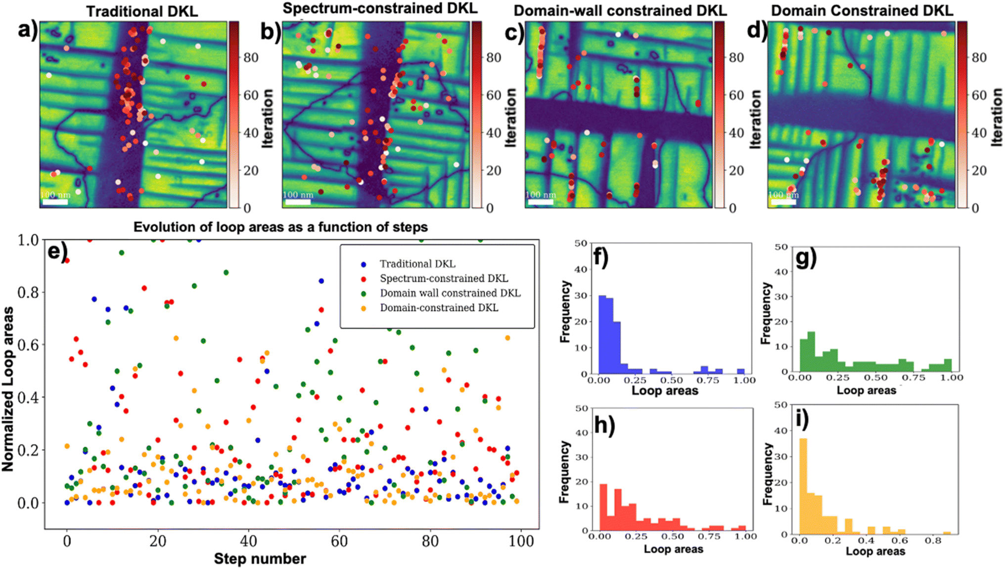Fig. 7 Constrained DKL in operating autonomous microscopy. (a)–(d) Sampled BEPS measurement locations of traditional DKL, spectrum constrained DKL, domain wall constrained DKL, and domain constrained DKL, respectively. (e) Hysteresis loop area as a function of DKL exploration steps. (f–i) Histograms of loop area distribution 1 of traditional DKL, spectrum constrained DKL, domain wall constrained DKL, and domain constrained DKL, respectively.

Fig. 7e plots the hysteresis loop areas as a function of exploration steps, with corresponding histograms showing loop area distributions in Fig. 7f–i. These loop area distributions indicate that traditional DKL tends to acquire closed hysteresis loops with loop areas close to zero, providing limited information regarding ferroelectric properties. However, gated-DKL samples more opening loops, resulting in deviated loop area distributions, indicating a more informative exploration process. Specifically, the live autonomous microscopy data show that the percentage of sampled opening loops with meaningful ferroelectric characteristics (open loop with a loop area >0.2) is 17% for the traditional DKL method, 48% for the gated-DKL with a spectrum constraint, 57% for gated-DKL with a domain wall constraint, and 22% for gated-DKL with a domain constraint. Additionally, it is worth mentioning that the reason the DKL samples a-domains is likely due to high uncertainty in those areas. Predicting spectra from certain locations can be challenging, leading to situations where model uncertainty does not significantly decrease with additional samples because the correlation between the structure and property is too low. The constrained methods help bypass these low-correlation areas, which are already known to be problematic, thus enhancing the efficiency of the sampling process.

Conclusions

In summary, we developed constrained active learning approaches that incorporate prior knowledge and specific interests for knowledge-informed active learning-driven autonomous experiments. In DKL-driven microscopy, prior knowledge can be applied to either the structural space or the spectral data. These workflows are fully operationalized on autonomous SPM systems and performance of traditional DKL and gated-DKL is compared. We demonstrated that constrained DKL can lead to more effective exploration in autonomous PFM experiments, via both pre-acquired datasets with known ground truth and operating autonomous PFM.

We note that the developed workflows can be represented as an example from single-step to multiple-step decision making. We expect that this approach can further be extended to build expert mixture gated workflows, where the role of the gate agent is to select the problem-appropriate DKL model, and the latter controls the exploration of image space. These multiple DKL models share the common training data but differ in possible reward functions and make different exploration decisions. This approach can be seamlessly extended to other microscopy and imaging techniques, accelerating scientific discovery. Furthermore, the constraint concept can be adapted for general Bayesian optimization in material discovery across a broad range of autonomous experimental fields.

Data availability

The constrained DKL approach developed in this work is publicly available at Github https://github.com/yongtaoliu/constrained_DKL.

Author contributions

Y. L. conceived the project, developed the constrained DKL approach, and wrote the manuscript. H. F. prepared the PTO sample. U. P. and Y. L. performed the analysis and measurement. All authors edited the manuscript.

Conflicts of interest

The authors declare no conflict of interest.

Acknowledgements

This work (gated-DKL development and PFM measurements) was supported by the Center for Nanophase Materials Sciences (CNMS), which is a US Department of Energy, Office of Science User Facility at Oak Ridge National Laboratory. U. P. and S. V. K. acknowledge support from the Center for Nanophase Materials Sciences (CNMS) user facility which is a U.S. Department of Energy Office of Science User Facility, project no. CNMS2023-B-02196. U. P. and S. V. K. acknowledge support from the high performance computing facility, ISAAC and Center for Advanced Materials and Manufacturing, the NSF MRSEC Center. H. F. acknowledges the support by the MEXT Program: Data Creation and Utilization Type Material Research and Development (JPMXP1122683430).

References

1. G. Binnig, C. F. Quate and Ch Gerber, Atomic Force Microscope, Phys. Rev. Lett., 1986, 56(9), 930–933.
2. G. Stan and S. W. King, Atomic force microscopy for nanoscale mechanical property characterization, J. Vac. Sci. Technol., B:Nanotechnol. Microelectron.:Mater., Process., Meas., Phenom., 2020, 38(6), 060801.
3. A. D. L. Humphris, M. J. Miles and J. K. Hobbs, A mechanical microscope: High-speed atomic force microscopy, Appl. Phys. Lett., 2005, 86(3), 034106.
4. M. Lanza, Conductive Atomic Force Microscopy, ed. Lanza M., Wiley, 2017.
5. W. Melitz, J. Shen, A. C. Kummel and S. Lee, Kelvin probe force microscopy and its application, Surf. Sci. Rep., 2011, 66(1), 1–27.
6. D. Kohl, P. Mesquida and G. Schitter, Quantitative AC - Kelvin Probe Force Microscopy, Microelectron. Eng., 2017, 176, 28–32.
7. A. Dazzi and C. B. Prater, AFM-IR: Technology and Applications in Nanoscale Infrared Spectroscopy and Chemical Imaging, Chem. Rev., 2017, 117(7), 5146–5173.
8. A. Dazzi, C. B. Prater, Q. Hu, D. B. Chase, J. F. Rabolt and C. Marcott, AFM–IR: Combining Atomic Force Microscopy and Infrared Spectroscopy for Nanoscale Chemical Characterization, Appl. Spectrosc., 2012, 66(12), 1365–1384.
9. Y. Seo and W. Jhe, Atomic force microscopy and spectroscopy, Rep. Prog. Phys., 2008, 71(1), 016101.
10. H. Watabe, K. Nakajima, Y. Sakai and T. Nishi, Dynamic Force Spectroscopy on a Single Polymer Chain, Macromolecules, 2006, 39(17), 5921–5925.
11. S. Jesse, A. P. Baddorf and S. V. Kalinin, Switching spectroscopy piezoresponse force microscopy of ferroelectric materials, Appl. Phys. Lett., 2006, 88(6), 062908.
12. Y. Liu, J. Yang, B. J. Lawrie, K. P. Kelley, M. Ziatdinov and S. V. Kalinin, et al., Disentangling Electronic Transport and Hysteresis at Individual Grain Boundaries in Hybrid Perovskites via Automated Scanning Probe Microscopy, ACS Nano, 2023, 17(10), 9647–9657.
13. R. K. Vasudevan, S. Jesse, Y. Kim, A. Kumar and S. V. Kalinin, Spectroscopic imaging in piezoresponse force microscopy: New opportunities for studying polarization dynamics in ferroelectrics and multiferroics, MRS Commun., 2012, 2(3), 61–73.
14. A. Ranjan, N. Raghavan, S. J. O'Shea, S. Mei, M. Bosman and K. Shubhakar, et al., Conductive Atomic Force Microscope Study of Bipolar and Threshold Resistive Switching in 2D Hexagonal Boron Nitride Films, Sci. Rep., 2018, 8(1), 2854.
15. Y. Liu, J. Yang, R. K. Vasudevan, K. P. Kelley, M. Ziatdinov and S. V. Kalinin, et al., Exploring the Relationship of Microstructure and Conductivity in Metal Halide Perovskites via Active Learning-Driven Automated Scanning Probe Microscopy, J. Phys. Chem. Lett., 2023, 14(13), 3352–3359.
16. S. V. Kalinin, M. Ziatdinov, J. Hinkle, S. Jesse, A. Ghosh and K. P. Kelley, et al., Automated and Autonomous Experiments in Electron and Scanning Probe Microscopy, ACS Nano, 2021, 15(8), 12604–12627.
17. M. Olszta, D. Hopkins, K. R. Fiedler, M. Oostrom, S. Akers and S. R. Spurgeon, An Automated Scanning Transmission Electron Microscope Guided by Sparse Data Analytics, Microsc. Microanal., 2022, 28(5), 1611–1621.
18. Y. Liu, K. Roccapriore, M. Checa, S. M. Valleti, J. Yang and S. Jesse, AEcroscopy: A Software–Hardware Framework Empowering Microscopy Toward Automated and Autonomous Experimentation, Small Methods, 2024, 8(10), 2301740.
19. Y. Liu, M. Checa and R. K. Vasudevan, Synergizing Human Expertise and AI Efficiency with Language Model for Microscopy Operation and Automated Experiment Design, 2024, available from: https://arxiv.org/abs/2401.13803.
20. Z. Diao, L. Hou and M. Abe, Probe conditioning via convolution neural network for scanning probe microscopy automation, Appl. Phys. Express, 2023, 16(8), 085002.
21. A. Krull, P. Hirsch, C. Rother, A. Schiffrin and C. Krull, Artificial-intelligence-driven scanning probe microscopy, Commun. Phys., 2020, 3(1), 54.
22. Y. Liu, K. P. Kelley, R. K. Vasudevan, W. Zhu, J. Hayden and J. Maria, et al., Automated Experiments of Local Non-Linear Behavior in Ferroelectric Materials, Small, 2022, 18(48), 2204130.
23. M. Ziatdinov, Y. Liu, K. Kelley, R. Vasudevan and S. V. Kalinin, Bayesian Active Learning for Scanning Probe Microscopy: From Gaussian Processes to Hypothesis Learning, ACS Nano, 2022, 16(9), 13492–13512.
24. O. Ovchinnikov, S. Jesse, S. Kalinin, H. Chang, S. Pennycook and A. Borisevich, Towards the Thinking Microscope, Microsc. Microanal., 2010, 16(S2), 160–161.
25. S. R. Spurgeon, C. Ophus, L. Jones, A. Petford-Long, S. V. Kalinin and M. J. Olszta, et al., Towards data-driven next-generation transmission electron microscopy, Nat. Mater., 2021, 20(3), 274–279.
26. J. Yang, A. V. Ievlev, A. N. Morozovska, E. Eliseev, J. D. Poplawsky, D. Goodling, et al., Coexistence and interplay of two ferroelectric mechanisms in Zn1-xMgxO, 2024, available from: https://arxiv.org/abs/2402.08852.
27. A. Raghavan, R. Pant, I. Takeuchi, E. A. Eliseev, M. Checa, A. N. Morozovska, et al., Evolution of ferroelectric properties in SmxBi1-xFeO3 via automated Piezoresponse Force Microscopy across combinatorial spread libraries, 2024, available from: https://arxiv.org/abs/2405.08773.
28. Y. Liu, S. S. Fields, T. Mimura, K. P. Kelley, S. Trolier-McKinstry and J. F. Ihlefeld, et al., Exploring leakage in dielectric films via automated experiments in scanning probe microscopy, Appl. Phys. Lett., 2022, 120(18), 182903.
29. S. V. Kalinin, C. Ophus, P. M. Voyles, R. Erni, D. Kepaptsoglou and V. Grillo, et al., Machine learning in scanning transmission electron microscopy, Nat. Rev. Methods Primers, 2022, 2(1), 11.
30. M. A. Rahman Laskar and U. Celano, Scanning probe microscopy in the age of machine learning, APL Mach. Learn., 2023, 1(4), 041501.
31. G. Volpe, C. Wählby, L. Tian, M. Hecht, A. Yakimovich, K. Monakhova, et al., Roadmap on Deep Learning for Microscopy, 2023, available from: https://arxiv.org/abs/2303.03793.
32. U. Pratiush, A. Houston, S. V. Kalinin and G. Duscher, Realizing Smart Scanning Transmission Electron Microscopy Using High Performance Computing, Rev. Sci. Instrum., 2024, 95(10), 103701.
33. U. Pratiush, K. M. Roccapriore, Y. Liu, G. Duscher, M. Ziatdinov and S. V. Kalinin, Building Workflows for Interactive Human in the Loop Automated Experiment (hAE) in STEM-EELS, arXiv, 2024, preprint, arXiv:2404.07381,  DOI:10.48550/arXiv.2404.07381.
34. S. V. Kalinin, Y. Liu, A. Biswas, G. Duscher, U. Pratiush and K. Roccapriore, et al., Human-in-the-Loop: The Future of Machine Learning in Automated Electron Microscopy, Microsc. Today, 2024, 32(1), 35–41.
35. Y. Liu, U. Pratiush, J. Bemis, R. Proksch, R. Emery, P. D. Rack, L. Yu-Chen, Y. Jan-Chi, S. Udovenko, S. Trolier-McKinstry, & S. V. Kalinin, Integration of Scanning Probe Microscope with High-Performance Computing: fixed-policy and reward-driven workflows implementation, arXiv, 2024, preprint, arXiv:2405.12300,  DOI:10.48550/arXiv.2405.12300.
36. B. N. Slautin, U. Pratiush, I. N. Ivanov, Y. Liu, R. Pant and X. Zhang, et al., Co-orchestration of multiple instruments to uncover structure–property relationships in combinatorial libraries, Digital Discovery, 2024, 3, 1602–1611.
37. B. Alldritt, F. Urtev, N. Oinonen, M. Aapro, J. Kannala and P. Liljeroth, et al., Automated tip functionalization via machine learning in scanning probe microscopy, Comput. Phys. Commun., 2022, 273, 108258.
38. M. Rashidi and R. A. Wolkow, Autonomous Scanning Probe Microscopy in Situ Tip Conditioning through Machine Learning, ACS Nano, 2018, 12(6), 5185–5189.
39. M. Ziatdinov, A. Ghosh, C. Y. Wong and S. V. Kalinin, AtomAI framework for deep learning analysis of image and spectroscopy data in electron and scanning probe microscopy, Nat. Mach. Intell., 2022, 4(12), 1101–1112.
40. M. Ge, F. Su, Z. Zhao and D. Su, Deep learning analysis on microscopic imaging in materials science, Mater Today Nano, 2020, 11, 100087.
41. F. Joucken, J. L. Davenport, Z. Ge, E. A. Quezada-Lopez, T. Taniguchi and K. Watanabe, et al., Denoising scanning tunneling microscopy images of graphene with supervised machine learning, Phys. Rev. Mater., 2022, 6(12), 123802.
42. K. Kimoto, J. Kikkawa, K. Harano, O. Cretu, Y. Shibazaki and F. Uesugi, Unsupervised machine learning combined with 4D scanning transmission electron microscopy for bimodal nanostructural analysis, Sci. Rep., 2024, 14(1), 2901.
43. Y. Liu, M. Ziatdinov and S. V. Kalinin, Exploring Causal Physical Mechanisms via Non-Gaussian Linear Models and Deep Kernel Learning: Applications for Ferroelectric Domain Structures, ACS Nano, 2022, 16(1), 1250–1259.
44. K. M. Roccapriore, Q. Zou, L. Zhang, R. Xue, J. Yan and M. Ziatdinov, et al., Revealing the Chemical Bonding in Adatom Arrays via Machine Learning of Hyperspectral Scanning Tunneling Spectroscopy Data, ACS Nano, 2021, 15(7), 11806–11816.
45. I. Sokolov, On machine learning analysis of atomic force microscopy images for image classification, sample surface recognition, Phys. Chem. Chem. Phys., 2024, 26(15), 11263–11270.
46. Y. Liu, K. P. Kelley, H. Funakubo, S. V. Kalinin and M. Ziatdinov, Exploring Physics of Ferroelectric Domain Walls in Real Time: Deep Learning Enabled Scanning Probe Microscopy, Adv. Sci., 2022, 9(31), 2203957.
47. K. M. Roccapriore, S. V. Kalinin and M. Ziatdinov, Physics Discovery in Nanoplasmonic Systems via Autonomous Experiments in Scanning Transmission Electron Microscopy, Adv. Sci., 2022, 9(36), e2203422.
48. Y. Liu, A. N. Morozovska, E. A. Eliseev, K. P. Kelley, R. Vasudevan and M. Ziatdinov, et al., Autonomous scanning probe microscopy with hypothesis learning: Exploring the physics of domain switching in ferroelectric materials, Patterns, 2023, 4(3), 100704.
49. Y. Meirovitch, C. F. Park, L. Mi, P. Potocek, S. Sawmya, Y. Li, et al., SmartEM: machine-learning guided electron microscopy, bioRxiv, 2023, available from: https://www.biorxiv.org/content/early/2023/10/08/2023.10.05.561103.
50. Y. Liu, K. P. Kelley, R. K. Vasudevan, H. Funakubo, M. A. Ziatdinov and S. V. Kalinin, Experimental discovery of structure–property relationships in ferroelectric materials via active learning, Nat. Mach. Intell., 2022, 4(4), 341–350.
51. S. Lu, B. Montz, T. Emrick and A. Jayaraman, Semi-supervised machine learning workflow for analysis of nanowire morphologies from transmission electron microscopy images, Digital Discovery, 2022, 1(6), 816–833.
52. C. K. Groschner, C. Choi and M. C. Scott, Machine Learning Pipeline for Segmentation and Defect Identification from High-Resolution Transmission Electron Microscopy Data, Microsc. Microanal., 2021, 27(3), 549–556.
53. X. Wang, J. Li, H. D. Ha, J. C. Dahl, J. C. Ondry and I. Moreno-Hernandez, et al., AutoDetect-mNP: An Unsupervised Machine Learning Algorithm for Automated Analysis of Transmission Electron Microscope Images of Metal Nanoparticles, JACS Au, 2021, 1(3), 316–327.
54. L. Yao and Q. Chen, Machine learning in nanomaterial electron microscopy data analysis, in Intelligent Nanotechnology, Elsevier, 2023, pp. 279–305.
55. Y. Liu, R. K. Vasudevan, K. K. Kelley, D. Kim, Y. Sharma and M. Ahmadi, et al., Decoding the shift-invariant data: applications for band-excitation scanning probe microscopy, Mach. Learn. Sci. Technol., 2021, 2(4), 045028.
56. Y. Liu, R. Proksch, C. Y. Wong, M. Ziatdinov and S. V. Kalinin, Disentangling Ferroelectric Wall Dynamics and Identification of Pinning Mechanisms via Deep Learning, Adv. Mater., 2021, 33(43), 2103680.
57. B. Alldritt, P. Hapala, N. Oinonen, F. Urtev, O. Krejci and F. Federici Canova, et al., Automated structure discovery in atomic force microscopy, Sci. Adv., 2020, 6(9), eaay6913.
58. S. Kang, J. Park and M. Lee, Machine learning-enabled autonomous operation for atomic force microscopes, Rev. Sci. Instrum., 2023, 94(12), 123704.
59. J. Sotres, H. Boyd and J. F. Gonzalez-Martinez, Enabling autonomous scanning probe microscopy imaging of single molecules with deep learning, Nanoscale, 2021, 13(20), 9193–9203.
60. S. Kandel, T. Zhou, A. V. Babu, Z. Di, X. Li and X. Ma, et al., Demonstration of an AI-driven workflow for autonomous high-resolution scanning microscopy, Nat. Commun., 2023, 14(1), 5501.
61. Y. Liu, M. A. Ziatdinov, R. K. Vasudevan and S. V. Kalinin, Explainability and human intervention in autonomous scanning probe microscopy, Patterns, 2023, 4(11), 100858.
62. M. Møller, S. P. Jarvis, L. Guérinet, P. Sharp, R. Woolley and P. Rahe, et al., Automated extraction of single H atoms with STM: Tip state dependency, Nanotechnology, 2017, 28(7), 075302.
63. O. M. Gordon, J. E. A. Hodgkinson, S. M. Farley, E. L. Hunsicker and P. J. Moriarty, Automated Searching and Identification of Self-Organized Nanostructures, Nano Lett., 2020, 20(10), 7688–7693.
64. R. A. J. Woolley, J. Stirling, A. Radocea, N. Krasnogor and P. Moriarty, Automated probe microscopy via evolutionary optimization at the atomic scale, Appl. Phys. Lett., 2011, 98(25), 253104.
65. O. M. Gordon and P. J. Moriarty, Machine learning at the (sub)atomic scale: next generation scanning probe microscopy, Mach. Learn. Sci. Technol., 2020, 1(2), 023001.
66. Robert Wolkow. 2 Rashidi et al. (43) Pub. Date : Publication Classification ( 54 ) System And Method For Autonomous Scanning Probe Microscopy With In-Situ Tip Conditioning, 2022.
67. A. Ghosh, B. G. Sumpter, O. Dyck, S. V. Kalinin and M. Ziatdinov, Ensemble learning-iterative training machine learning for uncertainty quantification and automated experiment in atom-resolved microscopy, npj Comput. Mater., 2021, 7(1), 100.
68. S. V. Kalinin, D. Mukherjee, K. Roccapriore, B. J. Blaiszik, A. Ghosh and M. A. Ziatdinov, et al., Machine learning for automated experimentation in scanning transmission electron microscopy, npj Comput. Mater., 2023, 9(1), 227.
69. S. V. Kalinin, M. Ziatdinov, S. R. Spurgeon, C. Ophus, E. A. Stach and T. Susi, et al., Deep learning for electron and scanning probe microscopy: From materials design to atomic fabrication, MRS Bull., 2022, 47(9), 931–939.
70. M. Ziatdinov, Y. Liu, and S. V. Kalinin, Active Learning in Open Experimental Environments: Selecting the Right Information Channel(s) Based on Predictability in Deep Kernel Learning, arXiv, 2022, preprint, arXiv:2203.10181,  DOI:10.48550/arXiv.2203.10181.
71. M. Valleti, R. K. Vasudevan, M. A. Ziatdinov and S. V. Kalinin, Deep kernel methods learn better: from cards to process optimization, Mach. Learn. Sci. Technol., 2024, 5(1), 015012.
72. Y. Liu, M. A. Ziatdinov, R. K. Vasudevan and S. V. Kalinin, Explainability and human intervention in autonomous scanning probe microscopy, Patterns, 2023, 4(11), 100858.
73. G. Narasimha, D. Kong, P. Regmi, R. Jin, Z. Gai, R. Vasudevan, et al., Multiscale structure-property discovery via active learning in scanning tunneling microscopy, 2024, available from: https://arxiv.org/abs/2404.07074.
74. B. N. Slautin, Y. Liu, H. Funakubo and S. V. Kalinin, Unraveling the Impact of Initial Choices and In-Loop Interventions on Learning Dynamics in Autonomous Scanning Probe Microscopy, J. Appl. Phys., 2024, 135(15), 154901.

---

Footnote

† This manuscript has been co-authored by UT-Battelle, LLC, under contract DE-AC0500OR22725 with the US Department of Energy (DOE). The US government retains and the publisher, by accepting the article for publication, acknowledges that the US government retains a nonexclusive, paid-up, irrevocable, worldwide license to publish or reproduce the published form of this manuscript, or allow others to do so, for US government purposes. DOE will provide public access to these results of federally sponsored research in accordance with the DOE Public Access Plan (http://energy.gov/downloads/doe-public-access-plan).

---