
 Open Access Article
 This Open Access Article is licensed under a Creative Commons Attribution-Non Commercial 3.0 Unported Licence
Balancing exploration and exploitation in de novo drug design
Maxime
Langevin
ab,
Marc
Bianciotto
 *b and
Rodolphe
Vuilleumier
*a
*b and
Rodolphe
Vuilleumier
*a
aPASTEUR, Département de Chimie, École Normale Supérieure, PSL University, Sorbonne Université, CNRS, 75005 Paris, France. E-mail: rodolphe.vuilleumier@ens.psl.eu
bMolecular Design Sciences – Integrated Drug Discovery, Sanofi R&D, 94400 Vitry-sur-Seine, France. E-mail: marc.bianciotto@sanofi.com
First published on 10th October 2024
Abstract
Goal-directed molecular generation is the computational design of novel molecular structures optimised with respect to a given scoring function. While it holds great promise for the acceleration of drug design, there remain limitations that hamper its adoption in an industrial context. In particular, the lack of diversity of molecules generated currently limits their relevance for drug design. Yet, most algorithms proposed focus solely on optimizing the scoring function, and do not address the question of diversity of the solutions they propose. Here, we propose a conceptual framework for analyzing the need for diverse solutions in goal-directed generation. Using a mean-variance framework, we present a simple model to bridge the optimization objective of goal-directed generation with the need for diverse solutions. We also show how to integrate it within different goal-directed learning algorithms.
Introduction
Goal-directed generation
De novo molecular design refers to the computational design of novel chemical structures. Recently, there has been renewed interest in de novo design, fueled in part by the popularity of AI generative models, which have been adapted to generate de novo molecular structures. De novo design tasks can be classified as either distribution learning tasks or goal-directed generation tasks.1 Distribution learning aims at generating large libraries of novel chemical structures, for instance in the aim of performing virtual screening. On the other hand, goal-directed learning aims at designing novel chemical structures that satisfy a desired molecular profile. This is done by generating structures that maximize a user-defined scoring function.1 In the context of industrial drug discovery, the scoring function S is designed to quantify whether a molecule fits to the drug discovery project's objectives. For instance, for a project in the lead optimization stage, the scoring function could combine predicted values for properties such as activity and selectivity on the target, as well as ADME-Tox properties. Existing goal-directed methods can be classified according to the molecular representation on which they operate2 – atom based, fragment based or reaction based, as well as the kind of optimization approach they use. The optimization approaches can be gradient-free, for instance population-based optimization algorithms such as genetic algorithms,3 swarm optimization4 or Bayesian optimization.5 They can also be gradient-based, where the generative model itself is updated through gradient descent. Gradient-based approaches rely heavily on reinforcement learning.6Diversity objective in goal-directed generation
Goal-directed learning is by essence framed as an optimization problem.1 This was stated in the work of Brown et al., who coined the term “goal-directed learning”, by using the following definition: “The goal is to find molecules that maximize the scoring function”. This objective translates in the algorithms used for goal-directed generation. In gradient-free approaches, the explicit objective is to maximize scores and to identify the highest scoring molecule. For gradient based approaches that resort to reinforcement learning, the reward is defined by the value of the scoring function at the end of an episode, during which a molecule was designed. As both the reward and the transition function are deterministic, the optimal policy is the one that puts the whole probability mass on the highest scoring molecule. This contrasts with the fact that an important objective in the different stages of drug discovery is often to provide diverse solutions. There is therefore an inherent conflict between the objectives of drug discovery (i.e., design high-scoring yet diverse molecules) and the formalism used by goal-directed generation (i.e., design the highest scoring molecules irrespective of their diversity). This was for instance noted in one of the early studies on goal-directed learning,7 which used a Long-Short Term Memory network (LSTM) on SMILES strings. The authors acknowledged that converging to a state where all the probability mass is placed on the top-scoring SMILES sequence is not desirable, even though it is the underlying objective of their reinforcement learning framework. To overcome this issue, they recommend that training should be stopped early in order to balance the design of high-scoring molecules with the design of structurally diverse ones. While it is possible, as proposed in the aforementioned work, to provide ad-hoc modifications of goal-directed learning in order to increase the diversity of generated molecules, a framework to reconcile goal-directed learning with the diversity objective still lacks. The main goal of this work is to propose such a framework and to reconcile the formalism used in goal-directed generation with the diversity objective. Furthermore, we also translate this framework in different goal-directed algorithms.Prior work on diversity in goal-directed learning
Diversity as an objective for generative models has been widely discussed for distribution learning,1,8 but less for goal-directed learning. In the field of optimization theory, a novel paradigm called quality-diversity9,10 has emerged in the last decade. This new paradigm states that optimizing ambitious objectives might not be achieved through direct optimization, which often leads to being stuck in local optima. Instead, quality-diversity proposes inclusion of novelty and diversity as inherent objectives. Counter-intuitively, this might lead to the discovery of solutions that perform better on the initial objective than directly optimizing the primary objective. This was applied to molecular design in a recent study,11 relying on the MAP-Elites algorithm.12 The search space is divided into different regions (called niches), and the optimization algorithm aims at finding optimal solutions for each niche, therefore enforcing diversity. Noteworthily, in this case diversity is only a means to an end and the final goal is still to find the highest scoring solutions. Other approaches have also been proposed: for instance, Liu et al.13 use a dual RNN framework to enforce exploration. One RNN is used to optimize the scoring function, while the other simply encodes a fixed probability distribution. During reinforcement learning, with some user defined probability, the second network can be used to sample some tokens. This prevents the optimization scheme from collapsing on the highest scoring sequences. Several other methods were proposed, some using a similar approach, as in Pereira et al.,14 or through a strategy which uses multiple agents concurrently.15 Finally, Blaschke et al.16 proposed the Memory-RL framework. Building on the REINVENT algorithm,7 they modified the scores in a similar way to MAP-Elites. The molecules generated are sorted in memory units. Closely related (e.g., based on Tanimoto similarity) molecules populate the same units, and when the number of molecules in a unit exceeds a predefined threshold, new molecules falling in that unit have their scores set to 0. This prevents the algorithm from exploring indefinitely the same region of chemical space.In this work, we present a novel theoretical framework that bridges the current formulation of goal-directed generation with a diversity objective. We first present this framework, and show how to apply it for different goal-directed generation algorithms in order to augment them with a diversity objective. We then present empirical results on different tasks for two datasets.
Theory
Probabilistic framework
The scoring function used in goal-directed learning is often designed to model the adequacy of a molecule to a drug discovery project. Nonetheless, many properties relevant to a drug discovery project are difficult to model accurately. Fig. 1 illustrates the life of a putative compound after de novo design. In order to reach the clinical stage of development, a molecule must face several challenges. First, it should be reasonably drug-like.17,18 It must also be synthesizable, in a reasonable number of steps and with limited cost. Then, the value predicted for the properties of interest have to be verified when tested in vitro in biochemical and cellular assays. Finally, even if it shows a good profile on the properties of interest, those only serve for proxies of the in vivo behavior of the molecule. Those uncertainties lead scoring functions to be imperfect predictors of a compound's future success in a drug discovery project. | ||
| Fig. 1 Challenges encountered after the design of a molecule. | ||
To account for this, we use a probabilistic framework. For a molecule, we define “success” as satisfying the pre-defined desired molecular profile. While scoring functions are imperfect, we assume that the probability of success for a given molecule m is an increasing function of its score:
| Psuccess(m) = f(S(m)) | (1) |
Generating batches of molecules
Another key point is that the output of generative design is generally not restricted to a single molecule. Rather, goal-directed algorithms are often used to generate a batch of molecules. Indeed, the Design–Make–Test–Analysis (DMTA) cycle19 in drug discovery rarely operates on a compound-by-compound basis, but rather by a batch of compounds. Given a budget n (i.e., a number of molecules to synthesize and test in one iteration of the DMTA cycle), the goal is to provide a batch M = (m1, m2, …, mn) of molecules. Switching to the generation of a batch of molecules is often done implicitly, by selecting the top n scorers from the pool of potential candidates identified by the goal-directed generation algorithm. This is for instance reflected in the goal-directed benchmarks of Guacamol,1 where the highest-scoring molecule is evaluated, as well as the top 10 and top 100 molecules. For a batch of n molecules, the outcome observed is a random vector (success (m1), success (m2), …, success (mn)) ∈ {0, 1}n. As the order of the molecules is interchangeable, we are actually only interested in the success rate:
In our probabilistic framework, the expected success rate is simply:
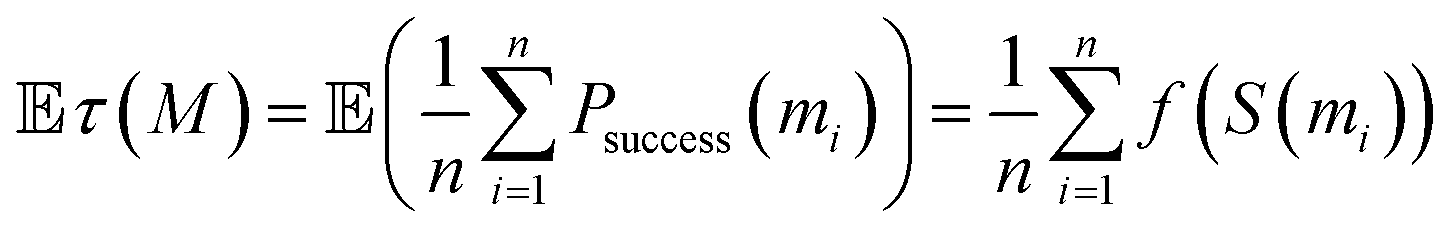
As f is an increasing function of the scoring function, maximizing this expectation is achieved by picking the top n scored molecules. Once again, at this stage, the best strategy remains to select a batch of the highest scoring molecules. This is due to the fact that the expectation is linear. Below, we will explore the fact that when we optimize a statistic that is not linear, but also depends on the correlation of molecules' outcomes, the optimal batch is one where molecules are not only high-scoring but also diverse.
Intuitively, selecting only the highest scoring molecules can be a risky strategy. Conceptually, the success of a molecule conditioned on its score depends on failure risks (e.g., failure of a predictive model, unmodeled properties, synthesizability issue). Assuming that these failure risks are shared by highly similar compounds (an assumption detailed in the following section), a de novo design approach that would generate closely related compounds is subject to a high risk of simultaneous failure of the generated molecules. This intuition is illustrated on the left of Fig. 2. Several scenarios are displayed, to illustrate our absence of knowledge of the landscape of the failure risks. On the other hand, a method that balances high scores with an inherent diversity objective (represented on the right of the figure) would mitigate those risks. This intuition will be formalized in the next section.
 | ||
| Fig. 2 De novo design of molecules subjected to an unknown failure risk, without diversity as an objective (left) and with diversity as an objective (right). Dots denote generated molecules. Red (respectively green) dots are subject (respectively not subject) to the failure risk of the corresponding scenario. Multiple scenarios are presented to illustrate that we ignore which failure risks molecules will face. | ||
Maximization of the expected success rate is a valid strategy, but not the only one available. Besides the rate of success, we might be interested in optimizing other statistics of the success rate. Indeed, statistics linked to the spread (e.g., the variance) of the distribution control the risk of the distribution. For instance, we can be interested in maximizing the probability P(τM > 0) of having at least one successful molecule, with the desired molecular profile. This is a more conservative strategy, which can correspond to a risk-adverse behavior.
Fig. 3 represents two hypothetical distributions describing the rate of success of a batch of molecules. The distribution on the left has a higher mean than the one on the right; on the other hand, its probability of having zero successes is far higher. In this situation, we might prefer sampling from the distribution on the right than from the distribution on the left, even though the latter has a higher expected success rate.
 | ||
| Fig. 3 Both panels represent hypothetical probability distributions on the rate of success of a batch of molecules. The expected rate of success is higher for the distribution in the left panel. On the other hand, the probability of having at least one success P(X ≥ 1) is higher for the distribution on the right panel. According to our overall goal, and our sensitivity to risk, we might privilege sampling from one distribution or the other. | ||
Mean–variance analysis
Here, we present several risk measures for probability distributions that can be of interest. It is to be noted that many risk measures were first described and implemented within the financial sector,20 to assess risks associated with financial portfolios. There is indeed a parallel between a financial portfolio and a batch of molecules selected to identify a drug candidate. In both cases, we observe a return which depends on the constituents of the portfolio or of the batch of molecules, and in both cases we are interested in avoiding realizations of the tail of the distribution. As we want to avoid the risk of a financial loss of high magnitude, we also want to avoid finding no successful molecules within our batch. One straightforward measure of risk is the variance var(X) =![[Doublestruck E]](https://www.rsc.org/images/entities/char_e168.gif) (X2) − (
(X2) − (![[Doublestruck X]](https://www.rsc.org/images/entities/char_e17b.gif) )2 of the underlying distribution. The variance is often tractable, and amenable to optimization.
)2 of the underlying distribution. The variance is often tractable, and amenable to optimization.
Intuitively, a higher variance stems from a more spread-out distribution, and thus a higher risk. This can be understood through the Chebyshev inequality:21 for a random variable X with mean (X) and finite variance σ, we have for any positive number α
 | (2) |
Applying it to the random variable τ(M), the probability of having no successful molecule P(τ(M) = 0) satisfies
 | (3) |
(τ(M)), as expected, or similarly lower the variance σ2.
Other risk measures include the value at risk,22 the conditional tail expectation23 and the expected shortfall.24 These risk measures give specific information on the tail of the distribution for which they are computed. On the other hand, specific optimization of these risk measures is often intractable.
Mean–variance analysis, also known as the modern portfolio theory, was introduced25 as a framework to mitigate risk in financial portfolios. Here, we transpose this analysis from selecting assets in a portfolio to selecting molecules to be tested in a DMTA cycle. The main idea of the mean–variance analysis is that we are not only interested in maximizing our mean return (in our case the success rate of our selected molecules), we are also interested in minimizing the variance of our return, as a proxy for risk.
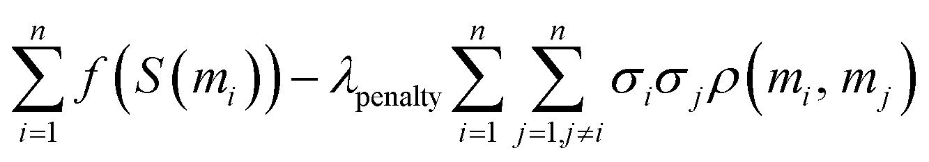
We propose an optimization objective allowing a trade-off between the variance and expectation value, optimizing both quantities in a single-objective framework through a weighted sum of both objectives, with a negative weight for the variance:
| (τ(M)) − λpenaltyσ2(τ(M)) | (4) |
As the variance of a sum of random variables {Xi}i=1n is the sum of covariances across all pairs, i.e., 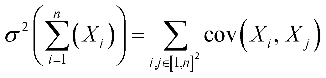 , we have:

We do not have direct access to the correlation coefficient ρ. While the score S(m) is assumed to model the single molecule probability of success, this probability is not independent between two molecules. To model correlation coefficients, we will rely on the well-known similarity principle in drug discovery.27
We thus choose to define a simplified correlation model based on Tanimoto similarity, as a step function given a threshold t:

The proposed objective eqn (4) can be rewritten:
 | (5) |
For the first part of the variance  , each individual term is increasing when f(S(mi)) goes from 0 to 1/2, and decreasing when f(S(mi)) goes from 1/2 to 1. Considering that we also (as it's our primary objective) want to maximize f(S(mi)), we can consider the latter case. Formally, one has f(S(mi))(1 − f(S(mi))) ≤ 1 − f(S(mi)) such that
 | (6) |
This allows us to simplify the overall objective by removing constant terms and redefining the free parameter λpenalty to yield the following objective:
In practice, we do not know f but expect practitioners to calibrate the scoring function such that its value reflects as accurately as possible the expected probability of success for a molecule. Using the correlation model introduced before, we can thus simplify this objective to derive our final optimization objective:
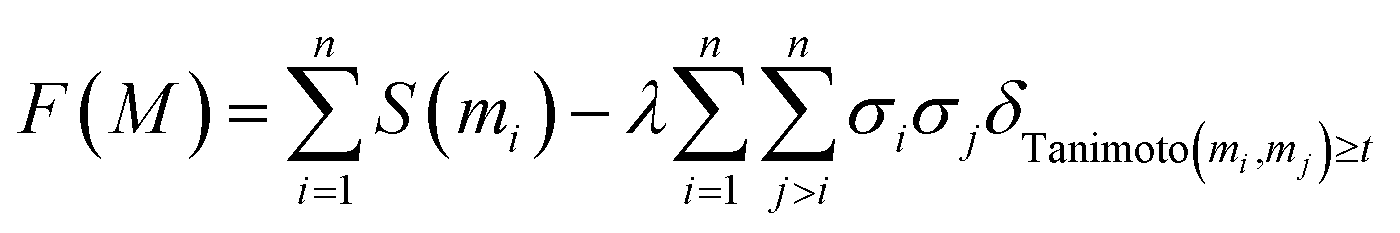 | (7) |
Materials and methods
Goal-directed generation of algorithms
In this section, we show how to modify goal-directed learning algorithms to include the optimization objective derived in eqn (7).Submodularity of the optimization objective. A submodular function f(M) over subsets M of a pool V is characterized26 by the property that for two sets M ⊂ V and N ⊂ V, with M ⊆ N, and an element m ∈ V\N (not in N) the function f satisfies the inequality:
| f(N ∪ {m}) − f(N) ≤ f(M ∪ {m}) − f(M). | (8) |
This property can be easily verified for the objective function F(M), eqn (7). Indeed, for a set M of molecules and a molecule m not in M, the discrete derivative F(M ∪ {m}) − F(M) is
 | (9) |
Thus, given another set N of molecules satisfying M ⊆ N, and for m not in N, we have
 | (10) |
Maximizing submodular functions with the constraint of a given budget of n molecules is a problem NP hard, but it has been shown that greedy approaches provide good approximations efficiently.26
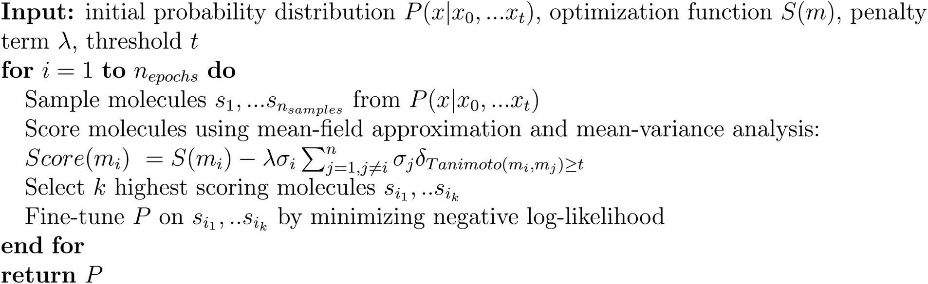
Greedy approach. The greedy approach for submodular functions adapted to our problem is described in Algorithm 1. In this greedy algorithm, we iterate on the number of molecules to select, re-scoring molecules using the penalty term computed over previously selected molecules at each iteration.

|
 | (11) |
Mean-field approximation. In these approaches, the probability of generating a molecule mi is independent with respect to the generation of a molecule mj so that the joint probability P(M) of generating an n-uplet of molecules M = (m1, …, mn) of molecules is simply
 | (12) |
The expectation of the objective function then reduces to
 | (13) |
Up to factors n and  this corresponds to a mean-field approximation in the expression of the objective function eqn (7), where the variance penalty term is replaced using this mean-field approximation:
 | (14) |
This formulation can be optimized with Monte-Carlo sampling and stochastic gradient descent. The mean-field approximation and the Monte-Carlo sampling allow computation of the cross-molecule penalty on molecules sampled from the current probability distribution Pθ, using other molecules from the same batch. The variance term acts as an entropy term favoring wide distribution with respect to peak distributions on a few best molecules. This promotes diversity among the generated molecules, which was our initial goal. It might seem that minimizing variance is in contradiction with maximizing diversity. In fact, variance minimization is done with respect to the score distribution, while diversity is promoted in molecular space. This is similar to taking the average of a set of random variables. If these random variables are highly correlated, the variance of the average is large for different trials, while the variance is lower if the random variables are uncorrelated.
The REINFORCE algorithm can be modified in a similar fashion, replacing the score by the objective (14), with the expectation taken over all other molecules from the batch.
Experimental setup
The main purpose of this work is to provide a theoretical framework for understanding the exploration–exploitation trade-off in goal-directed generation. Nonetheless, we also show experimental results for the HillClimb-MLE algorithm described above. We focus on this mean-field approach as it corresponds to a simple modification of existing REINFORCE algorithms and can thus be easily implemented in current packages.
|
Results
Diversity and scores of generated molecules
A first qualitative analysis is performed by visualisation of the results in low dimension. Fig. 4 shows the evolution over epochs of generated molecules on the DRD2 dataset without any similarity penalty. The generated molecules quickly collapse into a few narrow regions of the chemical space.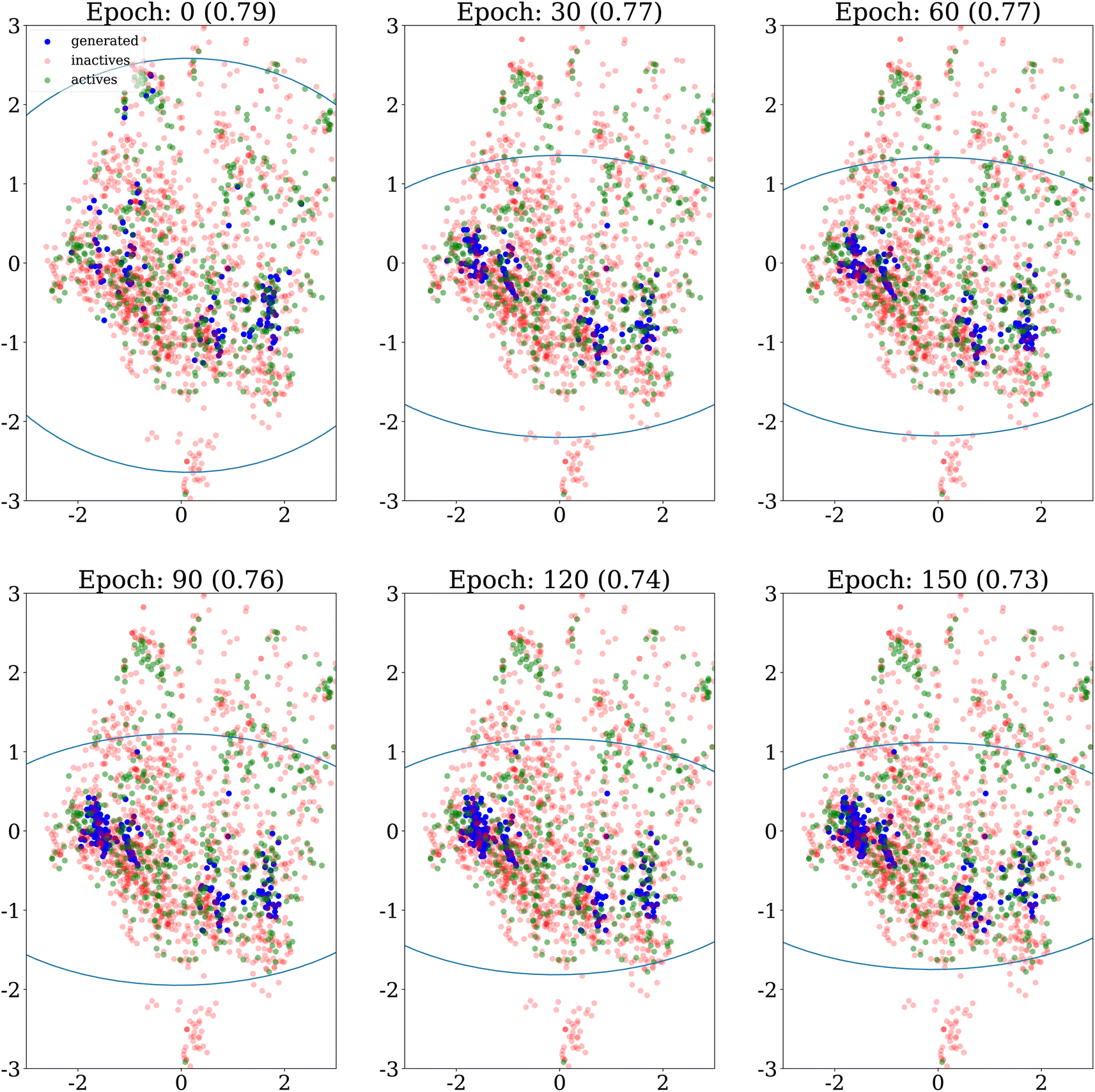 | ||
| Fig. 4 PCA projection of generated molecules with no similarity penalty (λ = 0), on the DRD2 dataset for different epochs, showing their evolution over time. The ellipses recover regions that span the 10th to 90th percentiles of the principal component values for the molecules generated up to the epoch considered. The internal diversity, indicated between parentheses, is computed as 1 minus the average Tanimoto similarity between ECFP4 fingerprints of generated molecules. | ||
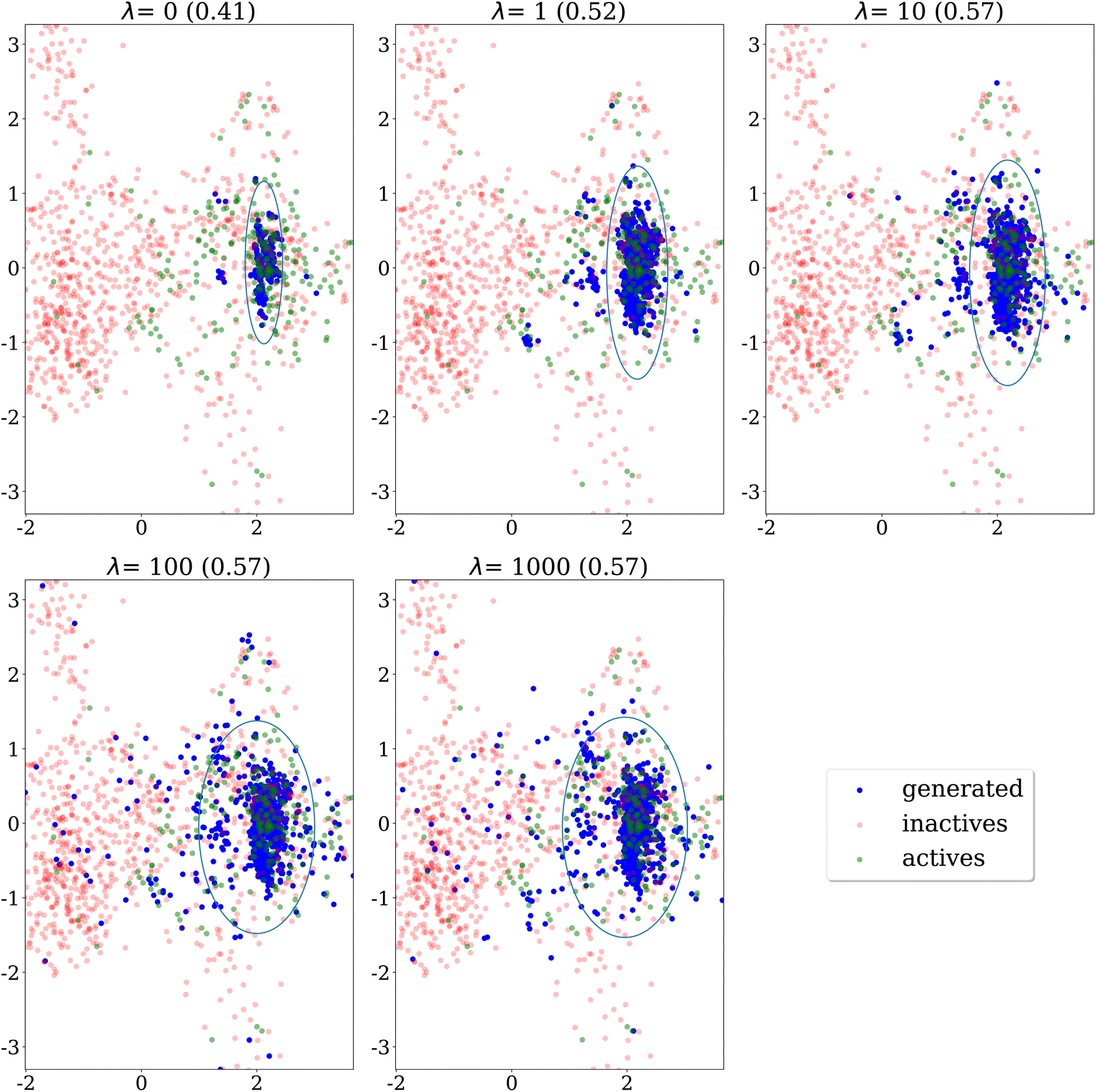
Fig. 5 shows PCA projection on the DRD2 dataset of molecules generated using Algorithm 2 with a similarity threshold of 0.7. We observe that as the λ penalty's value increases, the generative algorithm doesn't explore only the main cluster of actives, but also other regions of the chemical space covered by the dataset.
 | ||
| Fig. 5 PCA projection of molecules generated after 150 epochs using different values for the penalty λ, at a fixed similarity threshold 0.7, on the DRD2 dataset. The ellipses recover regions that span the 10th to 90th percentiles of the principal component values for the molecules generated up to the epoch considered. The internal diversity, indicated between parentheses, is computed as 1 minus the average Tanimoto similarity between ECFP4 fingerprints of generated molecules. | ||
Qualitative analysis of Fig. 6, which presents the same results on the EGFR dataset, yields a similar conclusion. The generated molecules cover a larger portion of the main cluster of actives as λ increases.
 | ||
| Fig. 6 PCA projection of molecules generated after 150 epochs using different values for the penalty λ, at a fixed similarity threshold 0.7, on the EGFR dataset. The ellipses recover regions that span the 10th to 90th percentiles of the principal component values for all generated molecules. The internal diversity, indicated between parentheses, is computed as 1 minus the average Tanimoto similarity between ECFP4 fingerprints of generated molecules. | ||
Finally, Fig. 7a and b show a heatmap of average similarities between generated sets on the DRD2 and EGFR dataset. As expected, internal similarity (represented by the diagonal) decreases as the variance penalty increases. An interesting observation is that the decrease is not constant, being stronger when λ is small. Even if λ evolves on a log-scale, the decrease in internal diversity becomes less pronounced for higher values of λ. This illustrates the tension between the two optimization objectives of eqn (7): at one point, decreasing the variance is too costly, and lowers too much the optimization scores, forcing the algorithm to find a good trade-off between the two.
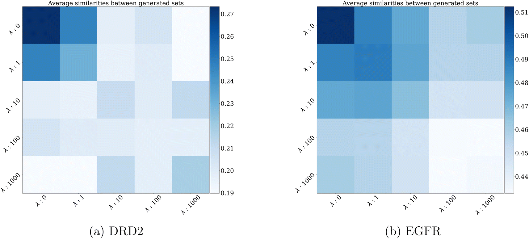 | ||
| Fig. 7 Internal Tanimoto similarities' heatmaps of generated molecule sets for different values of λ on the (a) DRD2 and (b) EGFR datasets. The sets of generated molecules are comprised of 128 molecules each. For comparison, average internal Tanimoto similarity is 0.16 for DRD2 and 0.15 for EGFR datasets. | ||
Trajectories of generated molecules
We also explore how the population of generated molecules evolve over the epochs. Coming back to Fig. 4, we show the PCA projection of generated molecules at different epochs when no similarity penalty is applied (λ = 0). As already noted, at the beginning (top left panel), the molecules cover the whole chemical space of the dataset, after the initial pretraining of the generative model. Quickly, the chemical space covered shrinks as the generative model focuses on the highest scoring regions.Fig. 8 shows the same evolution when the similarity penalty λ is set to 100. The generative model also converges to the highest scoring region but this is balanced by the similarity penalty. Eventually, the diversity objective prevents the generative model from collapsing to a few narrow regions of the chemical space.
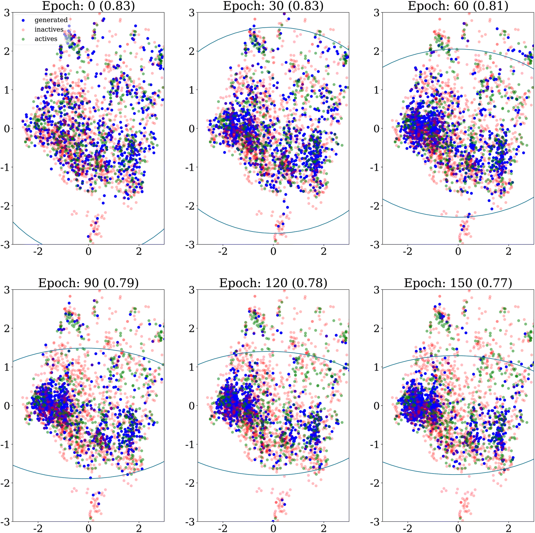 | ||
| Fig. 8 PCA projection of generated molecules with similarity penalty λ = 100, on the DRD2 dataset for different epochs, showing their evolution over time. The ellipses recover regions that span the 10th to 90th percentiles of the principal component values for all molecules generated up to the epoch considered. The internal diversity, indicated between parentheses, is computed as 1 minus the average Tanimoto similarity between ECFP4 fingerprints of generated molecules. | ||
Retrieval of active molecules
A good proxy for goal-directed algorithms is their ability to retrieve previously unseen actives. Fig. 9 shows the proportion of unseen actives (and analogs with a Tanimoto similarity ≥0.9) recovered for different values of λ on the DRD2 and EGFR datasets. This is shown both for each run individually (on the x-axis) and over the 10 runs (on the y-axis). Over 10 runs, as expected, the proportion of unseen actives recovered quickly increases with λ. Interestingly, it decreases for the highest value λ = 1000 for the EGFR dataset. Once again, this illustrates the exploration–exploitation trade-off: at one point, the increase in diversity is done at the expense of the optimization of predicted activities. On the DRD2 dataset, we see that less diversity (λ = 0 and λ = 1) leads to some retrieved actives on individual runs, but that number keeps being low when results are pooled over the 10 runs. This means that on this dataset, individual runs with higher diversity penalty might also generate a low number of actives, but as those actives are not the same between runs, taken together they represent a larger number of actives than for the runs with lower diversity penalty. This is particularly clear on the EGFR dataset where runs with less diversity find no actives, probably because the highest scoring region only contains very few actives. | ||
| Fig. 9 Proportion of actives and close analogs (with Tanimoto distance <0.9) recovered per run, and total for the set of 10 runs, for the DRD2 dataset (a) and the EGFR dataset (b), as a function of the λ penalty. | ||
Robustness to risk
The rationale on which we built our model and derived algorithms such as Algorithm 2 was that we assumed the presence of downstream risks that we could not model which could prevent our molecules from becoming drug candidates. To assess whether or not our diversity-oriented generation does give an edge in the case of unknown downstream risks, we designed a set of experiments, each testing the robustness of the generated molecules to a specific simulated downstream risk. After the generation, we selected at random a set of N molecules among the top 128 generated. To simulate what could happen in a realistic setting, molecules are judged successful if they meet the following conditions:• Sampling from a Bernoulli distribution parameterized with S(m) returns 1.
• m is not subject to a pre-specified risk.
We assess three different simulated downstream risks: one based on clustering, one based on the calculated coefficient partition clog![[thin space (1/6-em)]](https://www.rsc.org/images/entities/char_2009.gif) P and one based on the calculated total polar surface area (TPSA). These risks were selected to mimic risks where correlation is driven by structural similarity (clustering) and by property value (clogP and TPSA).
P and one based on the calculated total polar surface area (TPSA). These risks were selected to mimic risks where correlation is driven by structural similarity (clustering) and by property value (clogP and TPSA).
For the clustering simulated downstream risk, we perform a k means clustering on the initial dataset into 5 different clusters and select one of them at random. Molecules that do not belong to this specific cluster are considered as not successful. For the clogP simulated downstream risk, we select the clogP value of a training set's molecule at random. Then, we define an interval centered around this value, whose length is sampled uniformly in [1, 2] (Fig. 10).
 | ||
| Fig. 10 Illustration of how the clogP risk is computed: a molecule is selected at random in the dataset. An interval length is sampled uniformly in [1, 2]. The interval with this length, centered on the molecule's clogP value, defines the valid range of clogP values. When we sample a new molecule and a new interval length, the clogP risk changes, a process highlighted by the difference between the top and the bottom of the figure. The same principle is used for TPSA. | ||
A molecule whose clogP falls outside of this interval is not successful. We also perform a set of experiments using TPSA and the same procedure as with clogP, except that in this case the length of the interval is selected uniformly in [5, 10]. The metric we track is the probability of having at least one of the N molecules that is successful, i.e., its TPSA lies in the desired range. We choose this risk measure over variance, even though we explicitly optimize it over the latter. Indeed, our goal is to show that even with the simplification made in our model (e.g., choosing the variance as a risk measure as it allows for an analytical solution to be derived), we are still able to optimize with regard to more relevant risk measures.
For each simulated risk, we repeat the experiment 50 times, in order to imitate an unknown risk and to sample over the risk distribution. For the cluster-based simulated risk, the results as a function of λ are shown in Fig. 11a for the DRD2 dataset. We see that the probability of finding at least a molecule satisfying the TPP increases as λ increases from 0 to 100. As it forces the algorithm to generate more diverse compounds, the overall risk integrated over each experiment decreases. Nevertheless, if the variance penalty λ is set too high (here, λ = 1000), the probability of finding at least one molecule satisfying the TPP actually decreases, as we have already seen in Fig. 9. This illustrates once again the tension between diversity and optimization of the primary objective.
 | ||
| Fig. 11 Evolution of the probability of risk mitigation with λ as a function of N, the number of molecules selected among the generated ones. Heatmaps of the probability of finding at least one molecule satisfying the TPP (being active and in a predefined cluster: top left (a), activity and good value of clogP: top right (b), being in a predefined range of TPSA: bottom right (c)) as a function of λ for the DRD2 dataset and for the EGFR dataset (being in a predefined range of TPSA: bottom left (d)). | ||
For the clogP simulated risk, results integrated over 50 independent experiments are shown in Fig. 11b for the DRD2 dataset. Results are qualitatively similar to the experiment with the clustering risk; although the dependency of the outcome on λ is of a lower magnitude. Finally, results for the TPSA simulated risk are also displayed in Fig. 11c and d for both the EGFR and DRD2 datasets. We observe as well that the maximum probability of having at least one successful molecule increases with λ, before reaching a maximum for λ = 100.
Overall, results using those simulated downstream risks confirm that even with our model's limitations, the algorithm that derives from it still allows for a better minimization of a relevant risk measure for drug design. It also allows derivation of empirical values for the penalty λ. It is to be noted that all experiments were performed using Tanimoto similarity on ECFP4 fingerprints, with a threshold of 0.7. With other correlation models, it is possible that different results could be obtained.
Discussion
Analysis of the optimization objective
The final eqn (7) yields a simple optimization objective that gives a trade-off between exploitation of the highest scoring solutions (with the first term ) and exploration of diverse solutions (with the second term
  ). Noteworthily, λ is in fact the product between the initial penalty put on the variance in eqn (7), and of the correlation value ρ chosen in our simplified correlation model.
This model is interesting as it departs from the current paradigm described for goal-directed learning.1 It was indeed originally stated that “The goal-directed optimization of molecules relies on a formalism in which molecules can be scored individually”. While this is true when our primary objective is a linear combination of the outcomes of the selected molecules (such as the expected rate of success), this is not the case for other objectives (e.g., risk measures like variance of the distribution of the number of successes). For those objectives, if we assume correlation between the outcomes of molecules, they should not be scored individually but as a batch of molecules.
This model is appealing for its simplicity and the fact that it illustrates our intuitions regarding diversity. Nevertheless, it suffers from several limitations that are worth discussing. First, we assume that the variance is a good measure of risk. This choice is mainly made out of convenience, as it allows derivation of an analytical model. Ideally, a risk measure that specifically addresses the tail of the distribution could be of more interest. Indeed, the situation we really want to avoid is the one where none of the selected molecules meet the required endpoints. In this regard, minimizing a risk measure such as τ(M) = 0 would be more relevant to the problem at hand. Besides, we posit a simplified correlation model. To illustrate this point, we represent in Fig. 12 the relationship between the Tanimoto similarity of two molecules from the Sanofi database with known CYP3A4 inhibitory activity and the correlation coefficient between the random variables that indicate whether they are CYP3A4 inhibitors (activity ≤1 μM) or not. The dataset is comprised of all Sanofi internal data on small molecules profiled for CYP3A4 inhibition. We choose this property as it is often a liability that leads to discarding molecules in a drug discovery project. As we can see, the step function that we choose as a correlation model is a simplification of reality. On the other hand, we can see that it roughly models, in this case, the evolution of the correlation coefficient. As a general matter of fact, our correlation model assumes that the structure–activity relationship of properties impacting the downstream success of molecules is somewhat smooth on average. While activity cliffs30 (i.e., two very similar structures having drastically different properties) are a known reality for many properties of interest in drug design, this assumption is reasonable as we are interested in the average case. On the other hand, we cannot mitigate risks for which no well-defined structure–activity relationships exist.
 | ||
| Fig. 12 Correlation coefficient for being a cytochrome P450 3A4 inhibitor as a function of Tanimoto similarity on ECFP4 fingerprints. On the y-axis is the probability that a pair of molecules in the dataset with this level of similarity are both CYP3A4 inhibitors. | ||
Furthermore, as S(mi) → 1, the standard deviation σi tends to 0, limiting the impact of the penalty term. In the model, as S(mi) → 1, we become almost certain that the mi ∈ success. In practice, limitations of predictive models contradict this, and therefore setting a minimal value for the penalty term might be desired in numerical applications.
Comparison with existing methods
The goal of the experimental section is not to prove the experimental superiority of our algorithms, and a full comparison with existing methods is beyond the scope of our work. Furthermore, there are no clear benchmarks to compare algorithms that balance exploration and exploitation for molecular generation. That being said, we provide a quick qualitative comparison of Algorithm 2 with the MemoryRL algorithm.16 To decouple the impact of the generative algorithm from the diversity component, we re-implement MemoryRL's memory bucket within the same codebase as Algorithm 2 (Guacamol baselines). This could induce some changes as the authors originally implement it with the REINVENT algorithm,7 which is slightly different. , where n is the number of molecules sampled per epoch. This is assuming that we use Monte-Carlo sampling to compute the similarity penalty. Conversely, the algorithmic complexity of the similarity computation at epoch M for MemoryRL is
  . Indeed, the number of buckets (and therefore of similarity computation done for each of the n molecules sampled at a given epoch) grows as M × n. In our implementation (151 epochs, 1028 molecules per epoch, using a Nvidia Tesla K80 GPU), the runtime for MemoryRL on the DRD2 dataset is roughly 16 hours, while it is only 3 hours for Algorithm 2.
 | ||
| Fig. 13 PCA projection of generated molecules using different values for the penalty λ, at a fixed similarity threshold 0.7, on the DRD2 dataset with Algorithm 2, and with the MemoryRL algorithm.16 MemoryRL was run using a similarity threshold of 0.7, and a bucket size of 25 (as recommended by the authors). The ellipses recover regions that span the 10th to 90th percentiles of the principal component values for the generated molecules. The internal diversity, indicated between parentheses, is computed as 1 minus the average Tanimoto similarity between ECFP4 fingerprints of generated molecules. | ||
Fig. 14 shows the evolution of average scores throughout epochs for both methods: no major differences can be seen between both methods.
 | ||
| Fig. 14 DRD2: evolution of the average score throughout epochs for Algorithm 2 using different values for the penalty λ, at a fixed similarity threshold 0.7, and for the MemoryRL algorithm16 (bottom right). The envelope indicates the inter-run variability of the average score. | ||
Overall, no major differences in the results of both methods appear in this quick case study. The good trade-off between exploration and exploitation, and the best way to reach it, is problem dependent. Thus, we encourage the reader to test different algorithms to empirically identify the one most suited for their specific problem.
Conclusion
Throughout this work, we question the general framing of goal-directed learning. First, we highlight that we are generally interested in selecting batches of molecules, for which downstream success is uncertain. Then, we stress that maximizing our expectation is not necessarily what we want to achieve, and that other risk measures are of interest. Finally, assuming that the outcome of molecules is correlated for similar molecules, we show that scoring molecules individually is not correct, but that molecules should be scored by batch, taking into account inter-molecule correlations. This series of questions lead us to develop a model that explains the intuition behind the need for diversity for molecules generated by goal-directed learning algorithms. Within this model, we show how to modify goal-directed algorithms and especially the HillClimb-MLE approach to find a trade-off between exploration and exploitation of the scoring function.The experimental results are encouraging. Indeed, the algorithm is well behaved, and controlling the different parameters and modeling choices allow reasonable control of the outcome. On several simulated scenarios, we confirm our initial intuition: diversity mitigates unknown risk. This work is the opportunity to once again bridge the gap between requirements of a drug discovery project (which includes providing diverse solutions) and the current formulation of de novo molecular design.
Data availability
Code availability: All software to reproduce the results of this paper is available at: https://github.com/maxime-langevin/diverse_molecule_generation.Correlation coefficient for being a cytochrome P450 3A4 inhibitor: Circa 40k compounds with a measured pIC50 on CYP P450 3A4 inhibition were retrieved from Sanofi's internal data warehouse. Values were binarized to 1 if pIC50 > 6 and to 0 otherwise (compounds with an affinity stronger than 1 μM were thus considered as actives). For each pair of compounds, their Tanimoto similarity based on ECFP4 fingerprints was computed with the RDKit (using 2048 bits). For a given similarity value, the correlation coefficient is defined as the correlation coefficient of labels between pairs of compounds whose similarity lies in a small interval centered on the similarity value.
Datasets: The EGFR and DRD2 datasets were extracted from the ExCAPE-DB database33 and curated to discard structures appearing more than once or with extreme rule of five properties. The datasets' cleaning notebooks are included in the code repository.
Conflicts of interest
M. L. and M. B. are or have been employed by Sanofi and may hold shares and/or stock options in the company. The authors declare no other competing financial interest.Acknowledgements
The French National Association of Research and Technology (ANRT) is gratefully acknowledged for supporting M. L. (contract 2019/0821).References
- N. Brown, M. Fiscato, M. H. Segler and A. C. Vaucher, GuacaMol: Benchmarking Models for de Novo Molecular Design, J. Chem. Inf. Model., 2019, 59, 1096–1108 CrossRef CAS
.
- J. Meyers, B. Fabian and N. Brown, De novo molecular design and generative models, Drug Discovery Today, 2021, 26, 2707–2715 CrossRef CAS
- C. Steinmann and J. H. Jensen, Using a genetic algorithm to find molecules with good docking scores, PeerJ Phys. Chem., 2021, 3, e18 CrossRef
- R. Winter, F. Montanari, A. Steffen, H. Briem, F. Noé and D.-A. Clevert, Efficient multi-objective molecular optimization in a continuous latent space, Chem. Sci., 2019, 10, 8016–8024 RSC
- R. Gómez-Bombarelli, J. N. Wei, D. Duvenaud, J. M. Hernández-Lobato, B. Sánchez-Lengeling, D. Sheberla, J. Aguilera-Iparraguirre, T. D. Hirzel, R. P. Adams and A. Aspuru-Guzik, Automatic chemical design using a data-driven continuous representation of molecules, ACS Cent. Sci., 2018, 4, 268–276 CrossRef
-
R. S. Sutton and A. G. Barto, Reinforcement Learning: An Introduction, MIT Press, 2018 Search PubMed
- M. Olivecrona, T. Blaschke, O. Engkvist and H. Chen, Molecular de-novo design through deep reinforcement learning, J. Cheminf., 2017, 9, 1–14 Search PubMed
- W. P. Walters and R. Barzilay, Critical assessment of AI in drug discovery, Expert Opin. Drug Discovery, 2021, 16, 937–947 CrossRef CAS PubMed
- J. K. Pugh, L. B. Soros and K. O. Stanley, Quality diversity: A new frontier for evolutionary computation, Frontiers in Robotics and AI, 2016, 40 Search PubMed
-
J. Lehman and K. O. Stanley, Genetic Programming Theory and Practice IX, Springer, 2011, pp. 37–56 Search PubMed
- J. Verhellen and J. Van den Abeele, Illuminating elite patches of chemical space, Chem. Sci., 2020, 11, 11485–11491 RSC
- J.-B. Mouret and J. Clune, Illuminating search spaces by mapping elites, arXiv, 2015, preprint, arXiv:1504.04909, DOI:10.48550/arXiv.1504.04909.
- X. Liu, K. Ye, H. W. van Vlijmen, A. P. IJzerman and G. J. van Westen, An exploration strategy improves the diversity of de novo ligands using deep reinforcement learning: a case for the adenosine A2A receptor, J. Cheminf., 2019, 11, 1–16 CAS
- T. Pereira, M. Abbasi, B. Ribeiro and J. P. Arrais, Diversity oriented Deep Reinforcement Learning for targeted molecule generation, J. Cheminf., 2021, 13, 21 CAS
-
X. Hu, G. Liu, Y. Zhao and H. Zhang, De novo drug design using reinforcement learning with multiple GPT agents, Proceedings of the 37th International Conference on Neural Information Processing Systems, Red Hook, NY, USA, 2024 Search PubMed
- T. Blaschke, O. Engkvist, J. Bajorath and H. Chen, Memory-assisted reinforcement learning for diverse molecular de novo design, J. Cheminf., 2020, 12, 1–17 Search PubMed
- P. Renz, D. V. Rompaey, J. K. Wegner, S. Hochreiter and G. Klambauer, On failure modes in molecule generation and optimization, Drug Discovery Today: Technol., 2019, 32–33, 55–63 CrossRef
- M. Langevin, C. Grebner, S. Guessregen, S. Sauer, Y. Li, H. Matter and M. Bianciotto, Impact of Applicability Domains to Generative Artificial Intelligence, ACS Omega, 2023, 8, 23148–23167 CrossRef CAS PubMed
- A. T. Plowright, C. Johnstone, J. Kihlberg, J. Pettersson, G. Robb and R. A. Thompson, Hypothesis driven drug design: improving quality and effectiveness of the design-make-test-analyse cycle, Drug Discovery Today, 2012, 17, 56–62 CrossRef CAS
- P. Artzner, F. Delbaen, J.-M. Eber and D. Heath, Coherent measures of risk, Math. Finance, 1999, 9, 203–228 CrossRef
-
W. Feller and others, An Introduction to Probability Theory and its Applications, 1971 Search PubMed
-
N. D. Pearson, Risk Budgeting: Portfolio Problem Solving with Value-at-Risk; John Wiley & Sons, 2011 Search PubMed
-
P. Sweeting, Financial Enterprise Risk Management, Cambridge University Press, 2017 Search PubMed
- R. T. Rockafellar, S. Uryasev and others, Optimization of conditional value-at-risk, J. Risk, 2000, 2, 21–42 CrossRef
- H. Markowitz, Portfolio selection, J. Finance, 1952, 12, 77–91 Search PubMed
-
A. Krause and D. Golovin, in Tractability, ed. Bordeaux L., Hamadi Y. and Kohli P., Cambridge University Press, 1st edn, 2014, pp. 71–104 Search PubMed
-
Concepts and Applications of Molecular Similarity, ed. Johnson M. A. and Maggiora G. M., Wiley, 1991 Search PubMed
- Y. C. Martin, J. L. Kofron and L. M. Traphagen, Do structurally similar molecules have similar biological activity?, J. Med. Chem., 2002, 45, 4350–4358 CrossRef CAS
- H. Matter, Selecting optimally diverse compounds from structure databases: a validation study of two-dimensional and three-dimensional molecular descriptors, J. Med. Chem., 1997, 40, 1219–1229 CrossRef CAS PubMed
- G. M. Maggiora, On outliers and activity cliffs why QSAR often disappoints, J. Chem. Inf. Model., 2006, 46, 1535 CrossRef CAS PubMed
- J. H. Jensen, A graph-based genetic algorithm and generative model/Monte Carlo tree search for the exploration of chemical space, Chem. Sci., 2019, 10, 3567–3572 RSC
- N. Yoshikawa, K. Terayama, M. Sumita, T. Homma, K. Oono and K. Tsuda, Population-based De Novo Molecule Generation, Using Grammatical Evolution, Chem. Lett., 2018, 47, 1431–1434 CrossRef CAS
- J. Sun, N. Jeliazkova, V. Chupakhin, J.-F. Golib-Dzib, O. Engkvist, L. Carlsson, J. Wegner, H. Ceulemans, I. Georgiev, V. Jeliazkov and others, ExCAPE-DB: an integrated large scale dataset facilitating Big Data analysis in chemogenomics, J. Cheminf., 2017, 9, 1–9 Search PubMed
-
D. Neil, M. H. S. Segler, L. Guasch, M. Ahmed, D. Plumbley, M. Sellwood and N. Brown, Exploring Deep Recurrent Models with Reinforcement Learning for Molecule Design, Int. Conf. on Learning Representations, 2018 Search PubMed
| This journal is © The Royal Society of Chemistry 2024 |