
 Open Access Article
 This Open Access Article is licensed under a
 Creative Commons Attribution 3.0 Unported Licence
Operator-free HPLC automated method development guided by Bayesian optimization†
Thomas M.
Dixon
 a,
Jeanine
Williams
b,
Maximilian
Besenhard
c,
Roger M.
Howard
d,
James
MacGregor
e,
Philip
Peach
e,
Adam D.
Clayton
a,
Nicholas J.
Warren
a and
Richard A.
Bourne
*a
a,
Jeanine
Williams
b,
Maximilian
Besenhard
c,
Roger M.
Howard
d,
James
MacGregor
e,
Philip
Peach
e,
Adam D.
Clayton
a,
Nicholas J.
Warren
a and
Richard A.
Bourne
*a
aInstitute of Process Research and Development, School of Chemistry & School of Chemical Process Engineering, University of Leeds, Leeds, LS2 9JT, USA. E-mail: R.A.Bourne@leeds.ac.uk
bSchool of Chemistry, University of Leeds, Leeds, LS2 9JT, USA
cDepartment of Chemical Engineering, University College London, Torrington Place, London WC1E 7JE, UK
dPfizer Worldwide Research and Development, Groton, CT, USA
eDepartment of Analytical Research and Development, Pfizer Limited, Ramsgate Road, Sandwich CT13 9NJ, UK
First published on 14th June 2024
Abstract
The need to efficiently develop high performance liquid chromatography (HPLC) methods, whilst adhering to quality by design principles is of paramount importance when it comes to impurity detection in the synthesis of active pharmaceutical ingredients. This study highlights a novel approach that fully automates HPLC method development using black-box single and multi-objective Bayesian optimization algorithms. Three continuous variables including the initial isocratic hold time, initial organic modifier concentration and the gradient time were adjusted to simultaneously optimize the number of peaks detected, the resolution between peaks and the method length. Two mixtures of analytes, one with seven compounds and one with eleven compounds, were investigated. The system explored the design space to find a global optimum in chromatogram quality without human assistance, and methods that gave baseline resolution were identified. Optimal operating conditions were typically reached within just 13 experiments. The single and multi-objective Bayesian optimization algorithms were compared to show that multi-objective optimization was more suitable for HPLC method development. This allowed for multiple chromatogram acceptance criteria to be selected without having to repeat the entire optimization, making it a useful tool for robustness testing. Work in this paper presents a fully “operator-free” and closed loop HPLC method optimization process that can find optimal methods quickly when compared to other modern HPLC optimization techniques such as design of experiments, linear solvent strength models or quantitative structure retention relationships.
Introduction
Analytical High Performance Liquid Chromatography (HPLC) is used extensively in the pharmaceutical industry for quality control, reaction monitoring and quantitative analysis.1–3 Short method times are essential to increase the sampling rate for reaction monitoring or quality control purposes. Failure to obtain sufficient peak resolution can result in coelution of peaks, which is important to avoid for the accurate characterisation and quantification of impurities in the pharmaceutical industry to ensure regulations are met.2 Quantifying impurities ensures the manufactured Active Pharmaceutical Ingredients (APIs) are safe for human consumption through analysis of their pharmacological and toxicological properties, and will dictate if further purification or reaction condition modifications are required during the manufacture of the API.4 However, the ability to find HPLC methods that optimize for these parameters is costly due to the time and resources required to screen different conditions.HPLC methods separate analytes in a mixture based on their affinity for a stationary and a mobile phase. The technique is believed to separate between 60–80% of all existing compounds,5 making it the most used separation technique for the identification of impurities in the pharmaceutical industry.6 In addition, the method can be easily integrated as an online technique for monitoring reactions in flow.7 There is a demand for robust HPLC methods that give baseline resolution in the shortest amount of time, but the method development process can take several days for even the most experienced analytical chemists.
There have been many advancements in the efficiency of HPLC method optimization. Design of experiments (DOE) and modelling based method development tools are among the most popular.8,9 Software packages such as DryLab,10 ACD/LC Simulator11 and ChromSword12 aim to automate method development by selecting experiments based on different variations of DOE and offer tools such as peak tracking. Given data from a DOE, the retention time of each peak under different method conditions is fitted to a model. Using these models, a range of different method conditions can be simulated and the chromatogram quality assessed.13,14 Those conditions that match the desired qualities computationally are then run on the HPLC to give the optimal method. These models range from simple quadratics to linear solvent strength (LSS) models, which can be evaluated computationally to optimize parameters such as gradient steepness, isocratic hold times, pH or temperature. This methodology has also been used to automate robustness testing, ensuring baseline resolution in the chromatogram is maintained even with slight alterations in method conditions. Many examples have used this approach to optimize HPLC method conditions.15–21
Recent advancements in elution time prediction include in silico quantitative structure retention relationships (QSRR), that use machine learning models to map molecular fingerprints and molecular descriptors to retention times, so that molecules with unknown retention properties can be estimated using only their structures.22,23 This novel data driven optimization allows for information about ideal separation conditions to be obtained without needing to do any prior screening.
The main disadvantages with model-based approaches include the human processing time to label peaks and verify the models. The effectiveness of these models to simulate any secondary separation mechanisms or size exclusion effects can also lead to incorrect predictions.24 QSRR also requires large amounts of balanced datasets which are not always available. Although these methods can provide some automation, their functionality is not fully automated or closed-loop.
Operator-free optimization has shown to be successful in flow chemistry, where systems have been developed to be able to autonomously self-optimize input conditions such as residence time, equivalents and temperature to find optimal conditions for objectives such as yield, space-time yield and purity.25–32 These systems make use of optimization algorithms, which are most commonly used to optimize expensive-to-evaluate functions, where a considerable amount of computer processing or long experiment times are required. This can result in optimizing input conditions in fewer experiments compared to other machine learning techniques.33 As chemical reactions can take a significant amount of time to run, it makes them an ideal candidate for optimization algorithms.34 Provided a system can become “closed-loop”, where input conditions can be freely modified and objectives can be analyzed and interpreted automatically, an optimization algorithm can be integrated to fully automate finding optimal conditions. Therefore, the same approach can be used to optimize HPLC method conditions.
Berridge in 1986 stated that the use of optimization algorithms in HPLC method development is limited as they were previously only local and single-objective, one example being the Simplex algorithm.35,36 However recent advancements in optimization algorithms have increased their functionally to optimize globally and handle multiple objectives at once, making the concept of fully autonomous HPLC method optimization possible.34,37 Simplex was used to optimize for chromatogram quality.38,39 An iterative stochastic search, based on a pure random search where the design space is shrunk with each iteration, was also developed.40 However, both of these optimization approaches are unlikely to reliably find the global optimum in a HPLC method optimization.
Recent research has shown Bayesian optimization algorithms to be particularly efficient at solving complex optimization problems.41 They are described as being black box, meaning no previous intuitive knowledge about the optimization problem is required for them work.34 Therefore, other than developing a way to measure the chromatogram quality, no fundamental HPLC theory would need to be programmed to use these algorithms. This may offer an advantage when developing analytical methods on novel systems as no previous knowledge about the system would be assumed.
The use of Bayesian statistical modelling has been investigated by Lebrun et al. where multivariate models were used on experimental data to make predictions about retention time.42 A Bayesian design space has also been used for robustness testing for pharmaceutical assays.43 This work aims to incorporate Bayesian optimization algorithms as a means to find the global optima of chromatogram quality by changing method variables. One drawback of Bayesian modelling is that it does not scale well with problems containing 10–20 variables.44 However, HPLC method optimization should fit comfortably within the required dimensionality for this.
Boelrijk et al. demonstrated the use of Bayesian optimization algorithms to optimize HPLC methods for two complex dye mixtures in as few as 35 experiments.45 Both single and multi-objective optimization algorithms were used using input conditions that defined a multi-linear gradient program to separate the analytes, and custom objective functions such as ‘separation quality’ which combined the number of peaks detected with the method time. Building on this approach, we report herein the development of an autonomous impurity scouting method which focuses on achieving baseline resolution in the shortest time possible for full quantitative analysis.
Guidelines known as the Quality by Design (QbD) principles for liquid chromatography were written to ensure HPLC method conditions are explored effectively, ensuring impurities are identified and methods are robust.46 Coupling single and multi-objective Bayesian optimization algorithms with automated data analysis integrated into a closed loop optimization platform, offers a novel approach to HPLC method optimization. A schematic of this approach is described in Fig. 1. Work detailed in this paper aims to highlight the advancements of an industry 4.0 approach on HPLC method optimization, aiming provide a methodology that can be used automate and accelerate the identification of impurities in chemical reactions for the pharmaceutical industry.
 | ||
| Fig. 1 A schematic of the closed loop HPLC method optimization system. | ||
HPLC automation platform
An automated ‘closed-loop’ HPLC method optimization system was developed by writing some custom MATLAB code which could interface with macros in ChemStation. All HPLC methods, data analysis and generation of new conditions were performed autonomously, governed by an optimization algorithm. All the code has been made available on GitHub.47Input conditions
The design space of the optimization is defined by the lower and upper bounds of the three variables stated in Table 1, along with a description for each variable.| Variable | Description | Lower bound | Upper bound |
|---|---|---|---|
| Initial organic modifier concentration (%) | The organic modifier concentration when time is zero | 5 | 60 |
| Initial isocratic hold time/minutes | The length of time the initial organic modifier concentration is held for before a gradient method begins | 0 | 10 |
| Gradient time/minutes | The length of time from the initial organic modifier concentration to an organic modifier concentration of 95% after the initial isocratic hold | 1 | 10 |
Optimization algorithms and objective functions
The optimization algorithms used were: a single-objective Bayesian optimization algorithm with an adaptive expected improvement acquisition function (BOAEI), with the Gaussian process model using a ARD Matern kernel with V = 5/2;26,48 and a Thompson sampling efficient multi objective (TS-EMO) optimization algorithm.49,50 These algorithms are categorised as black box.For initialisation, the algorithms require an initial data set which is generated using Latin hypercube sampling (LHS).51 Seven initial conditions were generated using LHS for the three input variables defined in Table 1. A different set of seven initial LHS conditions were generated for each optimization experiment.
For the optimization algorithm to find conditions that maximize chromatogram quality, an objective function(s) must be defined. This can be done using a range of different chromatogram factors. One such factor is the separation between two peaks, known as resolution (Rs) which is defined in eqn (1). This factor denotes the separation between two Gaussian peaks, where tRx is the retention time of peak x and whx is the width of peak x at half height.
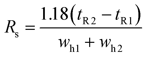 | (1) |
The larger the resolution between two peaks, the greater the separation. Perfect separation between two Gaussian peaks is achieved when Rs = 1.5. Separating all the peaks in a chromatogram with an Rs greater than 1.5 is optimal in most situations. The smallest overall Rs between any two consecutive pairs of peaks in a chromatogram is defined as the critical resolution (RsCrit) shown in eqn (2), where n is the number of consecutive peak pairs.
 | (2) |
An optimal HPLC method resolve all the analytes in a mixture with a RsCrit greater than 1.5 in the shortest possible time. Shorter method times are desirable to increase analysis throughput. Therefore, it was decided that the overall quality of the chromatogram would be governed by three factors: The number of peaks, the time the last peak elutes and RsCrit.
BOAEI was initially used to optimize HPLC method conditions. A weighted objective function (R) was created to represent the overall chromatogram quality based on these three HPLC factors. R is summarized in eqn (3), where N is the number of peaks detected and tRL is the retention time of the last peak in the chromatogram.
 | (3) |
As R tends towards zero, the chromatogram quality is increased. R = 0 denotes a chromatogram with seven peaks, RsCrit ≥ 2 and the time the last peak elutes at zero minutes. R = 1 denotes a chromatogram with zero peaks, RsCrit = 0 and the time the last peak elutes at 22 minutes. R will always be between zero and one. BOAEI will aim to minimize R by varying the three input variables defined in Table 1.
N, RsCrit and tRL are calculated from chromatogram data, normalized between 0 and 1 using pre-defined limits and then multiplied by a pre-defined weighting factor based on its importance. Each factor with its normalisation and weighting is described in Table 2. A special case for eqn (3) was also defined so when RsCrit > 2, the 0.3 ((2-RsCrit)/2) term is removed, preventing the term from becoming negative and from giving optimal values to chromatograms with large RsCrit values over N and tRL.
| Factor | Desired result | Normalisation | Weighting |
|---|---|---|---|
| Number of peaks (N) | Maximize | 0–7 | 0.6 |
| Critical resolution (RsCrit) | Greater than or equal to two | 0–2 | 0.3 |
| Time last peak elutes (tRL) | Minimize | 0–22 | 0.1 |
N was deemed the most important HPLC factor and so was given the largest weighting, followed by RsCrit and then tRL. Therefore, a 6![[thin space (1/6-em)]](https://www.rsc.org/images/entities/char_2009.gif) :3:1 ratio respectively of the weightings was selected to focus on this order of importance in the objective function. Normalisations were defined based on the maximum and minimum possible values that could be obtained for each objective in an experiment, based on the input variables defined in Table 1 and a mixture containing up to seven analytes. The selection of weightings is difficult without prior information about the system and can have a significant impact on the trajectory of the optimization.52 This is overcome with the multi-objective optimization approach, where the need to define weightings and normalisation parameters is removed.
:3:1 ratio respectively of the weightings was selected to focus on this order of importance in the objective function. Normalisations were defined based on the maximum and minimum possible values that could be obtained for each objective in an experiment, based on the input variables defined in Table 1 and a mixture containing up to seven analytes. The selection of weightings is difficult without prior information about the system and can have a significant impact on the trajectory of the optimization.52 This is overcome with the multi-objective optimization approach, where the need to define weightings and normalisation parameters is removed.
TS-EMO, a multi-objective Bayesian optimization algorithm, was next used with three objective functions. This time the HPLC factors defined in Table 2, N, RsCrit and tRL, were used individually as the different objective functions. The natural log of each objective was taken before it was fed into the optimization algorithm, as surrogate models tend to fit better to log transformed data.53 As TS-EMO aims to minimize its objective functions, the result of the log transformed N and RsCrit objectives were multiplied by −1, as these objectives are to be maximized. The TS-EMO optimization with three objectives is summarized in eqn (4).
| Minimize[−lnN, −lnRsCrit, lntRL] | (4) |
TS-EMO prioritizes solutions that maximize the hypervolume improvement of the design space. This makes use of Thompson sampling, an acquisition function that balances exploration of the design space versus exploitation of points that are believed to be optimal from the Gaussian process model, and NSGA-II, a genetic algorithm that uses Pareto ranking and crowding distance computations to find points that maximize the hypervolume improvement. The result is an algorithm that aims to find the trade-off between different objective functions. The points that lie on the boundary of the trade-off are described to be Pareto dominant and can be used to plot a Pareto front. This represents points in the design space for a given objective that cannot be improved without having a detrimental effect on another objective.34,50 Therefore, TS-EMO will aim to find the trade-off between N, RsCrit and tRL.
The optimization loop
The results from the initial conditions are processed and fed into the objective function(s) to calculate the objective(s). All the input conditions and the associated objective(s) is fed into the optimization algorithm selected to generate a new HPLC method, which is written to an excel file. A ChemStation macro reads the data written to excel and alters the HPLC method within ChemStation. After three minutes of equilibration at the newly defined conditions the HPLC method is started. Once the method has finished, the chromatogram data is read, and its quality is assessed by the selected objective function(s). The newly generated method condition along with the objective function(s) is concatenated with the other conditions and fed back into the optimization algorithm, where a new data point is generated. The cycle continues, each time with new data being acquired to aid in the search for the global optimum of the objective function(s). Fig. 1 shows a schematic of this process.Automated data analysis
The chromatogram datafiles were read and normalized between 0 and 200 before being processed by a Gaussian peak picking algorithm to automatically find the width and retention time for each peak detected.54Experimental section
Materials
Acetonitrile and toluene were analytical grade and purchased from Sigma-Aldrich. Ultrapure Water (18.2 MΩ) was obtained using a Millipore Gradient water purification system. Ammonium formate was purchased from Fluorochem. Thiourea, benzyl alcohol, toluene, benzophenone, naphthalene, biphenyl, anisole, benzaldehyde, phenol, benzyl benzoate and 4-nitrophenol were reagent grade and purchased from Sigma-Aldrich. All reagents were used without further purification.Sample preparation
The structures of these molecules are shown in Fig. 2.
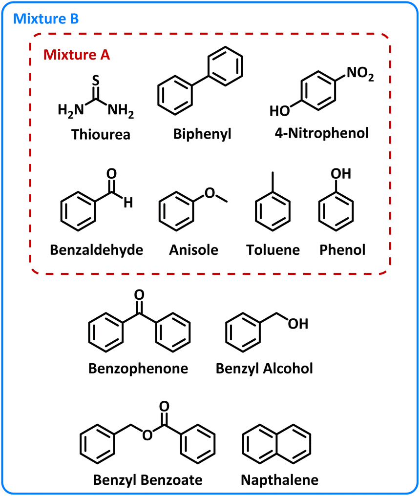 | ||
| Fig. 2 Molecular structures of the components within Mixture A (7 components) and Mixture B (11 components). | ||
Instrumentation
The liquid chromatography instrumentation used was an Agilent Infinity II HPLC that included a vial sampler, quaternary pump VL, diode array detector wide range and multicolumn thermostat. The instrumentation was controlled using ChemStation (version C.01.09 [144]). The chromatographic column used was an Agilent Poroshell 120 EC-C18 (50 mm × 4.6 mm, 2.7 μm) thermostated at 30 °C and buffered using the following solvent system: A = 10 mM ammonium formate in water, B = 10 mM ammonium formate in 9:1 acetronitrile:water. The flowrate was 1.5 mL min−1 and the injection volume was 2 μL. All methods finished at 95% B for two minutes and newly submitted methods were equilibrated for three minutes prior to starting. Detection was at 210 nm with a bandwidth of 2 nm.
MATLAB (version R2021b), Excel (office 365) and ChemStation (version C.01.09 [144]) were used to automate the HPLC method development process and were run on a HP Prodesk computer with an Intel® Core™ i5-8500 processor @ 3.00 GHz, 6 cores, and 8 Gb RAM.
HPLC optimizations
Nine optimizations were run in total. All the experimental data is available in the SI in Tables S1 to S9.† Traces for each optimization are also available in Fig. S6 to S8.† The design space for each optimization was defined according to Table 1.Results and discussion
A range of molecules containing chromophore groups and varying polarities were selected to test the effectiveness of the automated HPLC method optimization system, shown in Fig. 2. For Mixture A, seven molecules were selected including thiourea which is unretained on the C18 column used. Biphenyl is commonly used as an internal standard for quantitative analysis. Structurally similar compounds with different functional groups were selected to mimic the formation of a range of products in a standard reaction.BOAEI: single weighted objective optimization
Optimizations 1–3 used BOAEI and a weighted objective function R defined in eqn (3) to optimize for chromatogram quality on Mixture A. For a HPLC method to be labelled as ‘optimal’ for Mixture A, criteria were defined as N = 7, RsCrit ≥ 2, and tRL ≤ 6 minutes. These criteria were selected to allow for one minute of separation between each analyte peak and to ensure adequate baseline resolution. As R tends towards one, it represents a poorer quality HPLC method with a chromatogram that has a smaller N due to coelution, a smaller RsCrit from peak overlap and/or a longer tRL. As R tends towards zero, the opposite is true and will represent a chromatogram that is more likely to be deemed optimal. BOAEI will aim to minimize R by varying the input variables defined in Table 1. Optimizations 1–3 ran for 40 experiments overnight without interruption, facilitating usage during a time that would normally be instrument downtime. Fig. 3 shows the first chromatograms that satisfied the optimal criteria for each repeated optimization.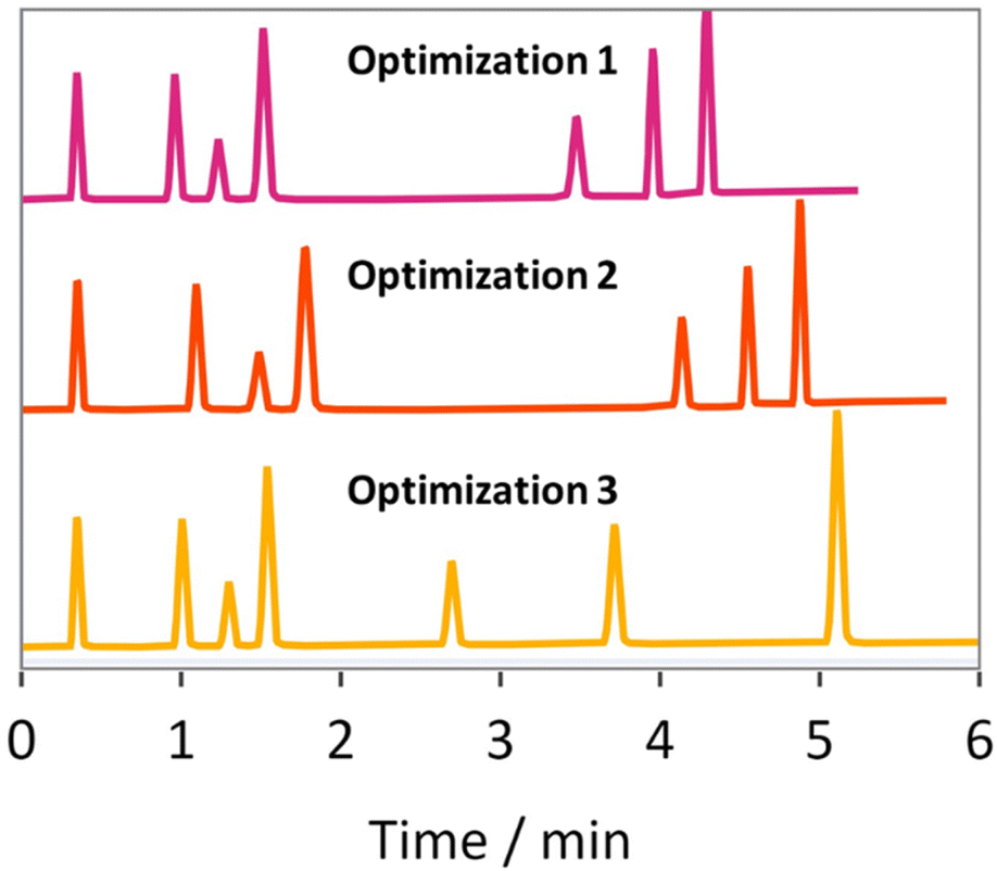 | ||
| Fig. 3 The first chromatograms from optimizations 1 (top), 2 (middle) and 3 (bottom) that satisfied the design space criteria (N = 7, RsCrit ≥ 2 and tRL ≤ 6 minutes), representing experiments 12, 19 and 9 respectively. | ||
BOAEI was able to find method conditions for optimizations 1–3 that satisfied the defined criteria in an average of 13 experiments. Experiments 12, 19 and 9 for optimizations 1–3 respectively were the first experiments to reach optimal conditions, achieving R values of 0.0195, 0.0222 and 0.0238 respectively.
Further experimentation resulted in even more optimal HPLC method conditions being discovered, where tRL was reduced to 3.9 minutes after 33 experiments (R = 0.0178), 3.3 minutes after 24 experiments (R = 0.0150) and 5.1 minutes after 28 experiments (R = 0.0230) for optimizations 1–3 respectively, which also satisfied the N = 7 and RsCrit ≥ 2 criteria. The design spaces for optimizations 1–3 are shown in Fig. 4 and have been plotted in a four-dimensional design space with R represented by a blue to green color scale (for 2D matrix plots see Fig. S9†). The crosses represent the first experiments to satisfy the design space criteria and correspond to the method conditions used to acquire the chromatograms in Fig. 3. The green stars represent the experiments with the smallest value of R achieved by each optimization. Despite more optimal conditions being found in later experiments, the algorithm was highly effective at finding the optimal regions of the design space in early experiments, demonstrated by the near overlap of the crosses and stars for each optimization in Fig. 4.
 | ||
| Fig. 4 The design spaces for optimizations 1–3 and the trade-off between RsCrit and tRL where N = 7. The color scale represents the value of the weighted objective function R. | ||
Fig. 4 shows that there are two optimal regions in the design space that lead to small values of R. The most optimal region lies with an initial organic modifier between 30 and 40%, a gradient time of one minute and the initial isocratic hold time between one and three minutes. The BOAEI algorithm in optimizations 1 and 2 found R to be minimized in this region of the design space. However, a second optimal region is observed when longer gradient times between six and ten minutes are selected, the initial isocratic hold time is close to zero minutes and the same initial organic modifier concentration is used. This is where the BOAEI identified R to be minimized in optimization 3.
The results from optimization 3 demonstrated that methods with long, shallow gradients, that allow the first four peaks to elute with a RsCrit ≥ 2, were just as optimal as methods with fast and steep gradients but with a longer initial isocratic hold time to enable efficient separation of the last three peaks, shown in optimizations 1 and 2.
Despite the success of BOAEI using R to find optimal chromatograms in as few as nine experiments, one drawback is demonstrated by the differences in the optimal chromatogram tRL after 40 experiments. The most optimal method condition found in optimization 2 had a tRL of 3.3 minutes, which is clearly more desirable than the most optimal methods in optimizations 1 and 3 which were only able to achieve 3.9 and 5.1 minutes respectively. Consequently, the R values are too similar for each optimal condition, with a difference of only 0.0043 between them. The weighting for the tRL term in R had a smaller influence on the overall value of R compared to the N and RsCrit terms, making the two regions in design space similarly optimal for the BOAEI algorithm.
Re-defining the individual weightings and normalisation factors for R may help to prevent this, however further experimentation and knowledge about the system being optimized would be required, which contradicts the aims of this research. Simply increasing tRL weighting could have other detrimental effects, such as favouring small tRL times over maximising N. Therefore, more complicated mixtures with unknown numbers of analytes may not be suitable for this type of optimization as an outside knowledge is required to compose an ideally suitable weighted objective function.
The trade-off between the RsCrit and tRL for optimizations 1–3 where N = 7 is also shown in Fig. 4. The red dashed box denotes the experiments that satisfied the design space criteria. A total of 13 experiments from optimizations 1–3 were found to satisfy these criteria. Most of the data points in the trade-off plot lie to the right-hand side where RsCrit is maximized. This is due to the RsCrit term in R having a larger weighting associated with it compared with the tRL term, so the BOAEI algorithm will focus on these methods more as the value of R is smaller.
The trade-off graph in Fig. 4 shows that if the critical resolution criteria were to be lowered to 1.5, a tRL of 2.05 minutes for the separation of Mixture A could be achieved, which was experiment 25 in optimization 2. R for this point is only 0.0694 as the R favours methods with RsCrit ≥ 2. For the algorithm to effectively explore methods with RsCrit ≥1.5 instead, the normalisation factors in R would have to be rewritten and the optimization repeated. A more suitable approach to optimising HPLC methods would involve an algorithm that removes the need for normalisation and weighting factors, and instead explores this trade-off. Therefore, it was decided that a multi-objective optimization algorithm such as TS-EMO, which is designed to effectively explore the trade-off between objectives such as N, RsCrit and tRL, would be more suitable. This Pareto front can then be used to select optimal conditions based on the user's requirements. It would also ensure that if the requirements ever changed, the optimization would not need to be repeated. Removing the weightings and normalisation factors would also mean less information about the mixture being optimized would be needed.
TS-EMO: multi-objective optimization
For optimizations 4–6 TS-EMO was used to optimize Mixture A. Three objective functions were constructed that dictated the overall quality of the chromatograms, defined in eqn (4). All three of these objectives were optimized for simultaneously, removing the need to define a custom weighted objective function. This makes using this HPLC method optimization system more applicable when working with mixtures with an unknown number of analytes.Optimizations 4–6 ran for 50 experiments each overnight without interruption. Fig. 5 shows the design space for all three of these optimizations overlayed (for 2D matrix plots see Fig. S10†), along with the trade-off between the RsCrit and tRL when N = 7, with the blue to orange color scale representing the distance to the Pareto front when RsCrit ≥ 1.5. This metric represents the smallest normalized distance of each point to the pareto front. Points that have RsCrit < 1.5 were deemed sub-optimal and so have been set to the maximum distance of 1. This metric aims to show the optimal conditions that are close in proximity to the pareto front so that they can be visualised in the design space clearly.
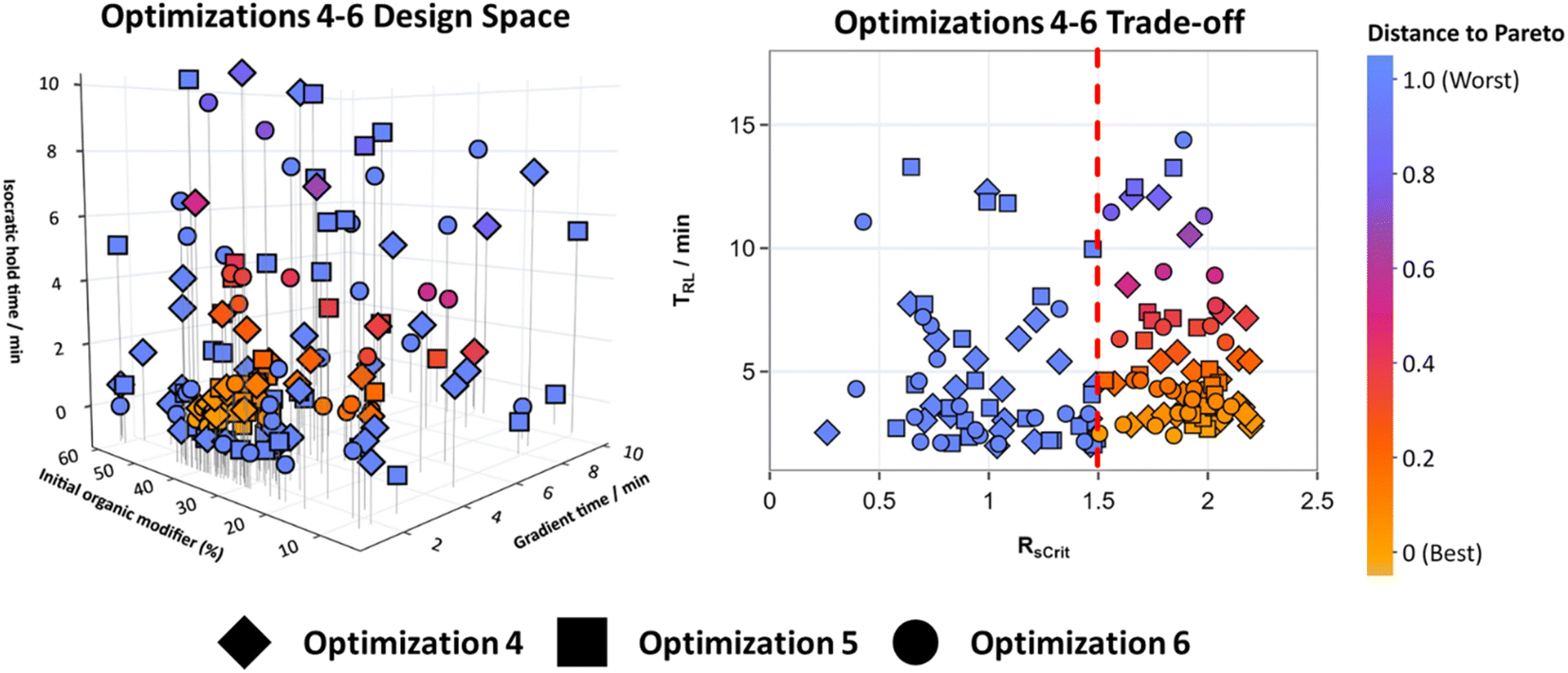 | ||
| Fig. 5 The design spaces for optimizations 4–6 and the trade-off between RsCrit and tRL where N = 7. The color scale represents the distance to Pareto front when RsCrit ≥ 1.5, represented by points to the right-hand side of the dotted line in the trade-off plot. | ||
Fig. 5 shows that the optimal HPLC method conditions for optimizations 4–6, that lie close to these best conditions, are in a very similar location of the design space compared to the method conditions where R is minimized for optimizations 1–3 in Fig. 4, showing that both algorithms were successful at effectively exploring the design space and identifying optimal conditions. As TS-EMO is a multi-objective optimization algorithm, it was efficient at finding points that lie close to the Pareto front between RsCrit and tRL when N = 7 in the trade-off graph in Fig. 5, unlike BOAEI in Fig. 4 where most of the data points in the trade-off graph were focused to the right-hand side with large RsCrit values.
The number of experiments required to reach an optimal method condition where N = 7, RsCrit ≥ 2, and tRL ≤ 6 minutes for optimizations 4–6, excluding the initial LHC, was 17, 40 and 22 respectively, making the average number of experiments required to reach the design space criteria, 26.3, over double the average of 13 experiments when compared to optimizations 1–3.
The overall best methods out of the 50 experiments for optimizations 4–6 were able to reduce tRL to 2.8 minutes after 17 experiments, 3.5 minutes after 44 experiments and 3.2 minutes after 22 experiments respectively, as well as satisfying N and RsCrit criteria. Although TS-EMO required more experiments, it outperformed BOAEI as it was able to consistently find more optimal HPLC method conditions with a smaller average tRL. It was additionally able to efficiently explore the Pareto front between RsCrit and tRL, which can be used to select chromatograms with other characteristics, such as methods with RsCrit ≥ 1.5, without the need to repeat the optimization. Therefore, if new design space criteria were to be defined as: RsCrit ≥ 1.5, N = 7 and tRL ≤ 6, the algorithm (excluding LHC experiments) was able to optimize the method conditions in as few as 11, 12 and 10 experiments for optimizations 4–6 respectively. The fastest overall experiment that satisfies these new criteria was experiment 32 in optimization 6 with tRL = 2.4 minutes. Given that in the pharmaceutical industry, methods need to undergo robustness testing, which is part of the QbD process for HPLC method development, the flexibility to change criteria without needing to repeat experimentation could be a useful time saving tool.
Some datapoints unfortunately in Fig. 5 were just below an Rscrit of 1.5 and therefore deemed sub-optimal. For example, experiment 31 in Optimization 4 had a tRL of 2.04 and an Rscrit of 1.46, which is very similar to experiment 25 in optimization 2 shown in Fig. 4, which had a tRL of 2.05 and Rscrit of 1.60. As TS-EMO aims to find the trade-off between objectives, conditions where RsCrit ≤ 1.5 were also explored, which may be undesirable. A constraint on the objective function could be added here to help reduce the number of experiments in this region and focus on more useful HPLC conditions.
To further test the effectiveness of using TS-EMO for HPLC method optimization, Mixture B which was a more complex mixture with 11 analytes was created. This mixture contained the same analytes as Mixture A but added four new molecules that were again varied in polarity and represented typical molecules found in reactions. The same design space that was used for optimizations 1–6 defined in Table 1 was selected to make the optimization process challenging, even though more molecules were present in Mixture B. Optimizations 7–9 ran for 50 experiments each, without interruption overnight. Fig. 6 shows the design space for all three of these optimizations overlayed (for 2D matrix plots see Fig. S10†), along with the trade-off between the RsCrit and tRL when N = 11, with the blue to orange color scale representing the distance to the Pareto front when RsCrit ≥ 1.5.
 | ||
| Fig. 6 The design spaces for optimizations 7–9 and the trade-off between RsCrit and tRL where N = 11. The color scale represents the distance to Pareto front when RsCrit ≥ 1.5, represented by points to the right-hand side of the dotted line in the trade-off plot. | ||
All three optimizations were unable to find HPLC method conditions that gave RsCrit ≥ 2, given the defined design space. Only a total of 12 experiments across optimizations 7–9 were found where RsCrit was greater than 1.5. Subsequently the design space criteria were redefined so RsCrit ≥ 1.5, N = 11 and tRL ≤ 10. This was first observed first for experiment 8 for Optimization 7 and experiment 10 for optimization 9. However, optimization 8 failed to find any optimal method conditions within 50 experiments. Points that were optimal appear to have their initial organic modifier concentrations between 5 and 35%, with short isocratic hold times and long gradient times, therefore most of the optimal conditions lie in the corner of this design space.
The randomness incorporated into selecting initial conditions using LHS may have been the reason why optimization 8 was unable to find any chromatograms that satisfied the design space criteria, when compared to optimizations 7 and 9. In this instance, using a 2k factorial DOE instead of LHS for initial conditions, where the corners of the design space are explored first, may have been more suitable as an initial starting point for TS-EMO to explore a wider range of conditions more quickly.
Extra experiments were run on optimization 8 and an optimal point was eventually found on experiment 68, which was significantly slower compared to optimizations 7 and 9, resulting in an average of 29 experiments across all three optimizations to satisfy the design space criteria. One experiment for optimization 8 was however able to reach an RsCrit of 1.48 by experiment 44, and located in a similar region of the design space to the optimal points in optimizations 7 and 9.
Despite few optimal chromatograms being discovered, the region of the design space that contains the optimal solutions is small. These experiments show that for more optimal solutions to be found, expansion of the design space, specifically changing the gradient time parameter to an upper bound of 15–20 minutes, may have enabled expansion of the Pareto front towards methods that give RsCrit ≥ 2. Selecting a suitable parameter space for the optimization will vary depending on the mixture being optimized. Generally, some prior knowledge about the mixture being optimized will be known. However, starting with a design space with a large range between variables and running an optimization will allow the user to see where the optimal points lie. This may be more beneficial to do before then reducing the range of the variables in the design space and repeating to fine tune more optimal conditions along the Pareto front.
Optimization 7 found the fastest tRL that satisfied the design space criteria, with separation in 5.2 minutes with an RsCrit of 1.58 by experiment 30. Optimal chromatograms for both Mixture A and Mixture B are shown in Fig. 7.
 | ||
| Fig. 7 Optimal chromatograms for Mixture A (top) and Mixture B (bottom) using TS-EMO, representing optimization 4 experiment 17 and optimization 7 experiment 30 respectively. | ||
Conclusion
This research has demonstrated the use of both BOAEI, a single objective optimization algorithm, and TS-EMO, a multi-objective optimization algorithm, to autonomously find HPLC method conditions that result in optimal chromatograms in as few as nine experiments for two different mixtures of analytes. Optimizations were run overnight with minimal interruption, making use of potential instrument downtime and alleviating method development during the working day so that increased focus on characterisation of peaks and robustness testing can be achieved, aiming to help accelerate impurity scouting during the manufacture of APIs.Further modifications to this software could include the implementation of discrete and continuous variable optimization algorithms to allow for different columns, pH's and solvents to be investigated, such as MVMOO.55 Defining desired input conditions and implementing custom written objective functions could enable the software to be used to optimize for methods across a range of different applications, including in the separation of polymers in GPC, proteins in size exclusion chromatography and for finding preparative HPLC conditions.
Data availability
All data from the optimisations is available in the electronic (ESI†). Code used for data analysis, graphics and the HPLC automation application is available via GitHub, details of which are also available in the ESI.†Author contributions
T. M. D. developed the automation platform, collected the experimental data, and wrote the manuscript. J. W. and J. M. for HPLC guidance and consulting. M. B., A. D. C, N. J. W. and R. A. B. for guidance in automation and Bayesian optimisation. R. M. H., J. M. and P. P. for industry input and advice. R. A. B. for securing EPSRC funding. P. P. and R. M. H. for securing industrial funding. P. P., R. M. H., A. D. C., N. J. W. and R. A. B. for conceptualisation. All authors were involved in reviewing and editing the manuscript and all approved the final version for submission.Conflicts of interest
There are no conflicts to declare.Acknowledgements
T. M. D. was supported by an EPSRC CASE award (EP/T517860/1) and Pfizer (2446912). R. A. B. was supported by the Royal Academy of Engineering under the Research Chairs and Senior Research Fellowships scheme. EPSRC also funded in part by EPSRC projects: EP/R032807/1, EP/V050990/1, EP/X024237/1. We thank Harriet A. M. Fenton for their contribution to artwork and Mary Bayana for research support.References
- M. R. Siddiqui, Z. A. Alothman and N. Rahman, Arabian J. Chem., 2017, 10, S1409–S1421 CrossRef CAS.
- D. Jain and P. K. Basniwal, J. Pharm. Biomed. Anal., 2013, 86, 11–35 CrossRef CAS PubMed.
- R. Nageswara Rao and V. Nagaraju, J. Pharm. Biomed. Anal., 2003, 33, 335–377 CrossRef CAS PubMed.
- F. Qiu and D. L. Norwood, J. Liq. Chromatogr. Relat. Technol., 2007, 30, 877–935 CrossRef CAS.
- M. W. Dong, HPLC and UHPLC for Practicing Scientists, John Wiley & Sons, 2nd edn, 2019 Search PubMed.
- M. Rodriguez-Zubiri and F.-X. Felpin, Org. Process Res. Dev., 2022, 26, 1766–1793 CrossRef CAS.
- C. J. Taylor, A. Baker, M. R. Chapman, W. R. Reynolds, K. E. Jolley, G. Clemens, G. E. Smith, A. J. Blacker, T. W. Chamberlain, S. D. R. Christie, B. A. Taylor and R. A. Bourne, J. Flow Chem., 2021, 11, 75–86 CrossRef CAS.
- L. Vera Candioti, M. M. De Zan, M. S. Cámara and H. C. Goicoechea, Talanta, 2014, 124, 123–138 CrossRef CAS PubMed.
- P. K. Sahu, N. R. Ramisetti, T. Cecchi, S. Swain, C. S. Patro and J. Panda, J. Pharm. Biomed. Anal., 2018, 147, 590–611 CrossRef CAS PubMed.
- Anon, Molnar Institute Dry Lab, 2021, http://molnar-institute.com/drylab/, accessed August 19th.
- Anon, ACD/Method selection suite, 2023, https://www.acdlabs.com/products/spectrus-platform/method-selection-suite/, accessed October 3rd.
- S. Galushko, I. Shishkina, E. Urtans and O. Rotkaja, 2018, pp. 53–94.
- H. J. G. Debets, J. Liq. Chromatogr., 1985, 8, 2725–2780 CrossRef CAS.
- E. J. Klein and S. L. Rivera, J. Liq. Chromatogr. Relat. Technol., 2000, 23, 2097–2121 CrossRef CAS.
- K. Monks, I. Molnár, H.-J. Rieger, B. Bogáti and E. Szabó, J. Chromatogr. A, 2012, 1232, 218–230 CrossRef CAS PubMed.
- A. H. Schmidt and I. Molnár, J. Pharm. Biomed. Anal., 2013, 78–79, 65–74 CrossRef CAS PubMed.
- B. Debrus, D. Guillarme and S. Rudaz, J. Pharm. Biomed. Anal., 2013, 84, 215–223 CrossRef CAS PubMed.
- I. Nistor, P. Lebrun, A. Ceccato, F. Lecomte, I. Slama, R. Oprean, E. Badarau, F. Dufour, K. S. S. Dossou, M. Fillet, J.-F. Liégeois, P. Hubert and E. Rozet, J. Pharm. Biomed. Anal., 2013, 74, 273–283 CrossRef CAS PubMed.
- L. Ferey, A. Raimbault, I. Rivals and K. Gaudin, J. Pharm. Biomed. Anal., 2018, 148, 361–368 CrossRef CAS PubMed.
- S. Karmarkar, X. Yang, R. Garber, A. Szajkovics and M. Koberda, J. Pharm. Biomed. Anal., 2014, 100, 167–174 CrossRef CAS PubMed.
- S. Fekete, V. Sadat-Noorbakhsh, C. Schelling, I. Molnár, D. Guillarme, S. Rudaz and J.-L. Veuthey, J. Pharm. Biomed. Anal., 2018, 155, 116–124 CrossRef CAS PubMed.
- X. Domingo-Almenara, C. Guijas, E. Billings, J. R. Montenegro-Burke, W. Uritboonthai, A. E. Aisporna, E. Chen, H. P. Benton and G. Siuzdak, Nat. Commun., 2019, 10, 5811 CrossRef CAS PubMed.
- R. Szucs, R. Brown, C. Brunelli, J. C. Heaton and J. Hradski, Int. J. Mol. Sci., 2021, 22, 3848 CrossRef CAS PubMed.
- M. J. Den Uijl, P. J. Schoenmakers, B. W. J. Pirok and M. R. Bommel, J. Sep. Sci., 2021, 44, 88–114 CrossRef CAS PubMed.
- A. D. Clayton, A. M. Schweidtmann, G. Clemens, J. A. Manson, C. J. Taylor, C. G. Niño, T. W. Chamberlain, N. Kapur, A. J. Blacker, A. A. Lapkin and R. A. Bourne, Chem. Eng. J., 2020, 384, 123340 CrossRef CAS.
- A. D. Clayton, E. O. Pyzer-Knapp, M. Purdie, M. F. Jones, A. Barthelme, J. Pavey, N. Kapur, T. W. Chamberlain, A. J. Blacker and R. A. Bourne, Angew. Chem., Int. Ed., 2023, 62, e202214511 CrossRef CAS PubMed.
- B. L. Hall, C. J. Taylor, R. Labes, A. F. Massey, R. Menzel, R. A. Bourne and T. W. Chamberlain, Chem. Commun., 2021, 57, 4926–4929 RSC.
- P. Mueller, A. Vriza, A. D. Clayton, O. S. May, N. Govan, S. Notman, S. V. Ley, T. W. Chamberlain and R. A. Bourne, React. Chem. Eng., 2023, 8, 538–542 RSC.
- C. P. Breen, A. M. K. Nambiar, T. F. Jamison and K. F. Jensen, Trends Chem., 2021, 3, 373–386 CrossRef.
- A. M. K. Nambiar, C. P. Breen, T. Hart, T. Kulesza, T. F. Jamison and K. F. Jensen, ACS Cent. Sci., 2022, 8, 825–836 CrossRef CAS PubMed.
- P. Jorayev, D. Russo, J. D. Tibbetts, A. M. Schweidtmann, P. Deutsch, S. D. Bull and A. A. Lapkin, Chem. Eng. Sci., 2022, 247, 116938 CrossRef CAS.
- C. J. Taylor, A. Pomberger, K. C. Felton, R. Grainger, M. Barecka, T. W. Chamberlain, R. A. Bourne, C. N. Johnson and A. A. Lapkin, Chem. Rev., 2023, 123, 3089–3126 CrossRef CAS PubMed.
- E. Brochu, V. M. Cora and N. d. Freitas, arXiv, 2010, preprint, arXiv:1012.2599, DOI:10.48550/arXiv.1012.2599.
- A. D. Clayton, J. A. Manson, C. J. Taylor, T. W. Chamberlain, B. A. Taylor, G. Clemens and R. A. Bourne, React. Chem. Eng., 2019, 4, 1545–1554 RSC.
- J. C. Berridge, Anal. Chim. Acta, 1986, 191, 243–259 CrossRef CAS.
- J. A. Nelder and R. Mead, Comput. J., 1965, 7, 308–313 CrossRef.
- J. L. J. Pereira, G. A. Oliver, M. B. Francisco, S. S. Cunha and G. F. Gomes, Arch. Comput. Methods Eng., 2022, 29, 2285–2308 CrossRef.
- N. Kuppithayanant, M. Rayanakorn, S. Wongpornchai, T. Prapamontol and R. L. Deming, Talanta, 2003, 61, 879–888 CrossRef CAS PubMed.
- S. Srijaranai, R. Burakham, R. L. Deming and T. Khammeng, Talanta, 2002, 56, 655–661 CrossRef CAS PubMed.
- Y. Dharmadi and R. Gonzalez, J. Chromatogr. A, 2005, 1070, 89–101 CrossRef CAS PubMed.
- E. G. Ryan, C. C. Drovandi, J. M. Mcgree and A. N. Pettitt, Int. Stat. Rev., 2016, 84, 128–154 CrossRef.
- P. Lebrun, B. Boulanger, B. Debrus, P. Lambert and P. Hubert, J. Biopharm. Stat., 2013, 23, 1330–1351 CrossRef PubMed.
- J. J. Peterson and M. Yahyah, Stat. Biopharm. Res., 2009, 1, 441–449 CrossRef.
- R. Moriconi, M. P. Deisenroth and K. S. Sesh Kumar, Mach. Learn., 2020, 109, 1925–1943 CrossRef.
- J. Boelrijk, B. Ensing, P. Forré and B. W. J. Pirok, Anal. Chim. Acta, 2023, 1242, 340789 CrossRef CAS PubMed.
- Anon, ICH Q8 (R2) Pharmaceutical development, 2021, https://www.ema.europa.eu/en/ich-q8-r2-pharmaceutical-development, accessed 17th Febuary.
- T. Dixon, HPLCMethodOptimisationGUI, 2024, https://github.com/Bourne-Group/HPLCMethodOptimisationGUI, accessed 10th January.
- R. Oldenhuis, FEX-GODLIKE, 2024, https://github.com/rodyo/FEX-GODLIKE/blob/master/GODLIKE.m, accessed 9th May.
- E. Bradford and A. Schweidtmann, Thompson sampling efficient multiobjective optimization, 2021, https://github.com/Eric-Bradford/TS-EMO, accessed 10th August Search PubMed.
- E. Bradford, A. M. Schweidtmann and A. Lapkin, J. Global Optim., 2018, 71, 407–438 CrossRef.
- R. L. Iman, J. M. Davenport and D. K. Zeigler, Latin Hypercube Sampling (Program User's Guide), United States Dep. NTIS, PC A05/MF A01. SNL English; Sandia Labs., Albuquerque, NM (USA), 1980 Search PubMed.
- D. E. Fitzpatrick, C. Battilocchio and S. V. Ley, Org. Process Res. Dev., 2016, 20, 386–394 CrossRef CAS.
- D. R. Jones, M. Schonlau and W. J. Welch, J. Global Optim., 1998, 13, 455–492 CrossRef.
- T. O'Haver, Peak Finding and Measurement, 2021, https://terpconnect.umd.edu/%7Etoh/spectrum/PeakFindingandMeasurement.htm, accessed 10th August.
- J. A. Manson, T. W. Chamberlain and R. A. Bourne, J. Global Optim., 2021, 80, 865–886 CrossRef.
Footnote |
| † Electronic supplementary information (ESI) available. See DOI: https://doi.org/10.1039/d4dd00062e |
| This journal is © The Royal Society of Chemistry 2024 |