Physics-driven discovery and bandgap engineering of hybrid perovskites

Abstract

The unique aspect of hybrid perovskites is their tunability, allowing the engineering of the bandgap via substitution. From the application viewpoint, this allows creation of tandem cells between perovskites and silicon, or two or more perovskites, with associated increase of efficiency beyond the single-junction Shockley–Queisser limit. However, the concentration dependence of the optical bandgap in hybrid perovskite solid solutions can be non-linear and even non-monotonic, as determined by band alignments between endmembers, presence of defect states and Urbach tails, and phase separation. Exploring new compositions brings forth the joint problem of the discovery of the composition with the desired band gap and establishing the physical model of the band gap concentration dependence. Here we report the development of the experimental workflow based on structured Gaussian Process (sGP) models and custom sGP (c-sGP) that allow the joint discovery of the experimental behavior and the underpinning physical model. This approach is verified with simulated datasets with known ground truth and was found to accelerate the discovery of experimental behavior and the underlying physical model. The d/c-sGP approach utilizes a few calculated thin film bandgap data points to guide targeted explorations, minimizing the number of thin film preparation steps. Through iterative exploration, we demonstrate that the c-sGP algorithm that combined 5 bandgap models converges rapidly, revealing a relationship in the bandgap diagram of MA_1−xGA_xPb(I_1−xBr_x)₃. This approach offers a promising method for efficiently understanding the physical model of band gap concentration dependence in binary systems, and this method can also be extended to ternary or higher dimensional systems.

---

Introduction

Organic–inorganic hybrid perovskites have gained significant attention in the field of materials science due to their superior properties and ease of manufacturability. These materials have shown remarkable progress in their power conversion efficiency (PCE), with advancements from 3.8% to 25.7% for single junction solar cells and above 30% for tandem perovskite and silicon solar cells.^1–3 This has generated considerable excitement, as perovskite materials hold the potential to replace traditional materials in various optoelectronic applications. Recent research has shown that compositional engineering by mixing cations and halides can exhibit improved performance compared to other alternatives.^4–7 However, these material advancements can come at the cost of stability issues. For instance, there may be decomposition of original precursor solutions or intrinsic halide segregation, leading to complex phase spaces.^8–11 The interplay of various components can give rise to complex behaviors across multicomponent phase diagrams, necessitating a more nuanced understanding of their properties. Nonetheless, the tuning of the bandgap and stability is of great interest in the field of optoelectronics. For instance, tandem solar cells benefit from bandgap engineering to optimize the absorption of light across different wavelengths, allowing a broader spectrum of light to be captured. Similarly, light emitting diodes (LEDs) rely on different bandgaps to produce a range of colors.^12–16 Understanding these properties is essential in optimizing the performances and stability of perovskite materials across a spectrum of applications.

The interplay of various endmembers can give rise to complex phase diagrams when looking at solid solutions with two and three phase regions. These various phases can lead to changes in bandgap evolution. For the bandgap, substitution on the A site in the perovskite structure with a chemical formula of ABX₃ (A = monovalent cations; B = divalent metal cations such as Pb²⁺ or Sn²⁺; X = halides) can directly lead to changes in the bandgap. For example, incorporating a larger or oversized A cation such as formamidinium (FA; ionic radius (r_A) = 256)^17,18 or dimethylammonium (r_A = 272 picometers (pm))¹⁷ compared to methylammonium (MA; r_A = 217 pm)^17,19 manifests smaller bandgaps of perovskites.^20–22 Substitution of I into Br or Cl can also lead to a bandgap increase.^23–25 However, some reports have shown that the size and geometry of the A cation can affect the bond length and angle between the B cation and X halide species,²⁶ which can also modulate the bandgap. In addition, substitution often also causes phase transitions and the bandgap can change abruptly at the structural phase transition boundaries.^20,27 These effects of the A, and X site substitution can give rise to complex behaviors across multicomponent phase diagrams broadly explored towards tunability and stability optimization. The bandgap-component dependence has been controversially reported,^28–33 which requires a better understanding of this relationship. It is also important to note that the optically determined bandgap can differ from the energy level landscape due to the potential presence of shallow defect levels, Urbach tails, and phenomena such as phase separation or chemical instability can compromise the effective bandgap.^34,35 These effects can be often identified from the photoluminescent and adsorption behaviors such as peak shapes.³⁶

MAPbI₃ has been widely used as a light absorber in perovskite solar cells, but it has shown to be unstable under ambient conditions due to the migration and electrochemical reaction of ions with the interface layer under operation conditions.^37,38 The movement of ions within the perovskite layer, especially lead ions can lead to the formation of defects and traps that can degrade the performance of the solar cell. To address this issue, larger organic cations such as FA or guanidinium (GA) have been added to MAPbI₃ in the MA sites, to mitigate the stability and ion migration.^39–41 This is due to the ability for a bulkier structure to provide steric hindrance making it harder for moisture to enter the crystal lattice, which can help stabilize the crystal structure preventing phase transitions and also hinder the migration of ions within the perovskite lattice. Tolerance factors have been used to forecast the stabilities of these modified perovskite structures. The tolerance factor of the MAPbI₃ perovskite is ∼0.91, which deviates from 1, suggesting that its crystal structure is distorted from the ideal cubic structure.⁴² The r_A of GA (278 pm)¹⁷ is larger than that of MA (217 pm),⁴¹ which reduces crystal distortion and increases the tolerance factor, resulting in improved long-term stability.^40,41,43

Synthesis methods can be broadly categorized into manual and high-throughput approaches. Manual synthesis involves hand-crafted processes, often resulting in the creation of one sample at a time. In contrast, high-throughput synthesis automates the creation of multiple samples, significantly accelerating the study of materials and their properties. Machine Learning (ML) methods offer the advantage of predicting the composition dependence of the bandgap, reducing the number of samples required. With a known physical model that predicts this composition dependence, the desired composition can be easily determined. If the concentration space is explored using high-throughput synthesis, a physical or non-parametric model can be derived from the experimental data.

Though high-throughput synthesis is quicker than manual methods, which can be time-consuming due to its sequential nature, neither model nor data are typically available at the outset of an experiment. The aim then becomes determining both within a minimal experimental budget. This challenge arises in both manual and high-throughput synthesis contexts. While manual approaches can feasibly explore 1- or 2-dimension (D) parameter spaces (such as binary or ternary phase diagrams), automated synthesis can tackle 2–4 D spaces through batch updates. It is important to note, however, that methods like grid search and data-driven Bayesian Optimization (BO) can be limited to higher dimensions.

Recently, we have demonstrated that the introduction of the mean function representing the physical behavior of the system allows for accelerating the BO optimization and joint discovery of the physical model and materials optimization during the active experiment.⁴⁴ In this study, we utilize the structured Gaussian Process (sGP) approach to investigate the bandgap diagram of the MA_1−xGA_xPb(I_1−xBr_x)₃ binary system. The selection of this system as our subject is due to its intriguing material properties and the notable size difference between GA (ionic radius = 278 pm)⁴¹ and MA ions (ionic radius = 217 pm).⁴⁵ This size disparity is believed to influence lattice structures and interactions, potentially affecting the electronic properties, such as the bandgap. The variability in bandgap energies observed when mixing MAPbI₃ and GAPbBr₃ provides a comprehensive test bed for evaluating the adaptability and accuracy of the sGP model. Furthermore, the impact of GA on the stability and photovoltaic performance of the material adds another layer of complexity, making this system a focal point for both theoretical and experimental exploration in the field of perovskite research. By leveraging the sGP model, we aim to not only predict bandgap behaviors but also to establish correlations with performance metrics, thus facilitating a systematic investigation that enhances our understanding and optimization of material properties through compositional engineering. This iterative approach of synthesis and testing based on model predictions is expected to expedite the discovery of optimal compositions and deepen insights into the underlying mechanisms influencing these advanced materials. The general workflow, illustrated in Fig. 1, begins with preparing several thin films for inclusion in the sGP algorithm. From there, the algorithm suggests new points for synthesis and measurement, repeating this cycle until the physical model is elucidated and optimization opportunities are identified.

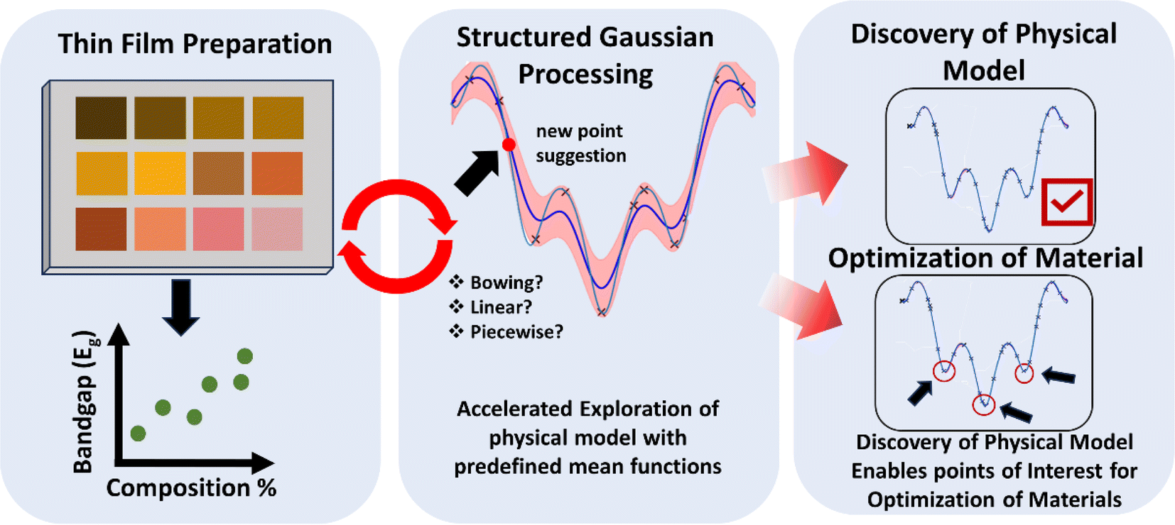Fig. 1 Workflow for discovery of the physical behavior of the bandgap of a mixed perovskite system.

Discussion

The Gaussian Process (GP) represents a general class of non-parametric methods for reconstructing functions from noisy observations.^46–48 In the classical GP setting, it is assumed that the behavior of the system over a certain parameter space x is given by the ground truth function f(x). This function is unavailable for observers. However, available for observers are the measurements, y_i at the chosen points x_i. It is assumed that the relationship between the measurements and the function is given by y_i = f(x_i) + noise, where the noise term is assumed to follow specific (usually Gaussian) distribution. The primary aim of GP is to reconstruct the function f̂(x) from these observations, providing not only the estimate of f(x) but also quantifying the uncertainty σ(x) and characterizing the noise. The reconstructed function f̂(x), hereafter referred to as f̂(x), represents our best estimate of the true function based on available data.

The fundamental assumption in the GP method is that the values of the function f̂(x) across the parameter space are correlated, and the correlations are described by the kernel function. The kernel function is assumed to have a certain functional form, for example squared exponential or Matern. For these functions, the kernel is characterized by a parameter vector corresponding to the characteristic length scale, and these kernel parameters are learned self-consistently from the data jointly with the noise. Over the last few decades, more complex correlation structures represented by kernel functions have been extensively explored. However, the characteristic aspect of classical GP methods is that the mean value of the prior function is zero.⁴⁹ Classically, this assumption is made based on the perceived lack of domain specific prior knowledge of system behavior over the parameter space.

The unique aspect of GP models is that they can be used as a foundational framework for active learning methods, e.g., for the development of optimal measurement strategies. In Bayesian Optimization (BO), the predicted function and its uncertainty are combined in the acquisition function balancing the expected gain and potential to discover useful behaviors in weakly explored parts of the parameter space. To accomplish this goal, the human operator suggests the policy balancing the prediction f̂(x) and uncertainty (σ(x)), of the surrogate function. BO is typically implemented as myopic optimization, meaning that the policy is used to plan only the next experimental step, and is implemented as an acquisition function. For example, in the greedy approach the next measurement point is chosen as argmax (f(x)), i.e., the strategy aims to discover the maximum of the function. Alternatively, in a pure exploration policy, argmax (σ(x)) is chosen as the next measurement point to minimize the uncertainty of the system fastest. Other acquisition functions such as expected improvement (EI) or upper confidence bound (UCB) balance uncertainty and optimization. Note that BO allows for fully probabilistic methods as well, where the search point is drawn from the full posterior distribution (Thompson sampling).

Over the last three years, GP and BO have become the techniques of choice for guiding automated experiments in areas as diverse as materials synthesis,^50–52 automated microscopy,^53–55 and other instrumental methods.^56–58 However, the BO methods based on pure GP are data-driven, meaning that the surrogate model is based purely on data and does not take into account the (partially) known physics of the system. In comparison, the classical physical paradigm will rely on constructing the predictive model based on the expected physics of the system, starting with the linear approximation, and proceeding to more complex descriptions if evidenced by data.

Recently, we proposed that addition of the probabilistic mean function to the GP can significantly accelerate the discovery.^44,59 Here, we construct the mean function that represents the possible physics of the process, including the functional form and the priors on parameter distributions. We note that in physical experiments the operator typically has a good idea on the possible prior distributions, either from the previously published work or domain-specific knowledge. The update of the model then updates both the kernel and noise parameters, and the distribution of the model parameters. This approach can be further extended to the scenarios when several models of system behavior, e.g. several structured models and potentially zero mean model, are available, as exemplified in hypothesis learning.^59,60 The three possible mean functions that are initially defined are linear, quadratic and piecewise, and the use of these models will be denoted as using the default sGP functions (d-sGP). Regardless, the actual physical model d-sGP should be able to discover the ground truth better than the GP algorithm. Furthermore, creating custom mean functions with prior knowledge of physical models can also further accelerate the discovery process. This is where a custom sGP mean function (c-sGP) can be implemented. Note that in sGP, the physical model is learned during the active experiment along with materials optimization.

With sGP, we can further define several tasks for Bayesian optimization, namely minimizing the model parameter uncertainty, discovering the right model, achieving the desired bandgap value, or maximizing/minimizing the bandgap. Here, we first illustrate the discovery of the unknown function using GP-based active learning. The underpinning principle of all Bayesian methods is to start with some initial beliefs on the system (priors), acquire data and update beliefs given from the data to get posteriors. The posteriors can be used to estimate the unknown function and its uncertainty. The active learning in GP is realized by creating the acquisition function that balances the estimated function and uncertainty into a single discovery policy (exploration–exploitation tradeoff).

The important aspect of the GP methods is their sensitivity to the initial priors defined before the experiment. While often irrelevant for long experimental sequences when intrinsic properties of the data generation process are discovered, this consideration becomes preponderantly important for short experimental budgets. For a simple GP, the initial parameters for a defined functional form of the kernel include the kernel length scale or lateral scale of correlations in the system, scale (vertical scale), and noise prior. Here, we illustrate the discovery process of the sufficiently complex 1D function using different combinations of these parameters.

The ground truth function is characterized by multiple local minima, accompanied by a noisy component (0.01) (Fig. 2a and b). The noise prior encompasses the combined effect of our confidence in the precision of our measurements and any uncontrollable factors that might influence the measurements. Similarly, the kernel length scale reflects our belief regarding the potential variation in the properties of the system. If we possess accurate assumptions regarding the noise prior and kernel length, the experimental process can be expedited and simplified. This allows the GP algorithm to rapidly converge towards the ground truth (Fig. 2a).

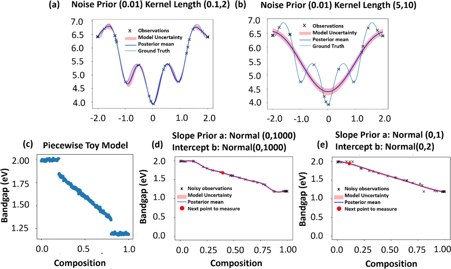Fig. 2 (a and b) GP with different noise priors and kernel lengths: (a) GP discovery with noise prior (0.01) and kernel length (0.1, 2) (b) GP discovery with noise prior (0.01) and kernel length (5, 10). More results about the effect of noise prior and kernel length on GP discovery at various steps can be found in Fig. S3.† (c–e) Effect of priors on sGP discovery: (c) piecewise toy model data for the sGP experiment. (d) sGP discovery with slope prior a = normal (0, 1000), intercept b = normal (0, 1000) (b) sGP discovery with slope prior a = log normal (0, 1), intercept b = normal (0, 2). More results about the effect of priors on sGP discovery at various steps can be found in Fig. S4.†

Conversely, if we establish a prior with incorrect or inflexible assumptions, the convergence of the algorithm with the ground truth becomes unattainable. As the algorithm persists in compensating for its inability to accurately describe the ground truth, it eventually loses faith in the provided measurements (Fig. 2b). While GP has the potential to uncover the ground truth given appropriate priors, sGP incorporates a constructed mean function that represents the plausible physics underlying the ground truth. Consequently, sGP facilitates quicker convergence by leveraging this additional information.

In the GP algorithm, the availability of prior data such as prior noise, kernel length, and kernel scale plays a crucial role in reconstructing the function and estimating its uncertainty. However, this process heavily relies on the experimenter's intuition regarding the experiment and its anticipated outcome. The GP algorithm can only discover the true underlying function if the chosen priors enable it to do so. Furthermore, the selection of priors can also influence the number of exploration steps required to converge to the ground truth. To evaluate the performance of the d-sGP mean functions, we examine piecewise toy model data as shown in Fig. 2c. This model exhibits an evolution in the bandgap, like the conditions observed during alloy formation. Specifically, when the variable “x” is small (x < 20% or x > 80%), no alloy is formed. In this model, there exist two regions where alloy formation does not occur, providing us with test cases to assess the convergence capabilities of d-sGP mean functions in capturing the ground truth. Initially, the model is presented with only two data points to make its determination, followed by a total of 30 exploration steps. We anticipate that a more effective model will exhibit a faster decrease in the overall uncertainty within the system.

d-sGP requires the incorporation of physics or domain knowledge to effectively model a system. However, it is important to exercise caution when employing priors devoid of physical foundations, as blind adherence to such priors can lead to prolonged experimental timelines. In our investigation (Fig. 2d and e), we utilized a linear mean function (y = a × x + b) to explore the toy data.

In the first exploration, the model prior for the slope coefficient (a) was assigned to a large variance (0, 1000) for indicating a normal distribution centered around 0 with a standard deviation of 1000. The prior for the intercept (b) was defined as a normal distribution (0, 1000), favoring larger intercept values. Upon commencing a 30-step exploration, as shown in Fig. 2d, we observed that the algorithm initially relied on the given priors and failed to discover areas where alloy formation did not occur before step 20. However, after surpassing this threshold, the algorithm progressively disregarded the priors and embarked on a more comprehensive exploration of the system. It is worth noting that priors should not be perceived as optimization objectives, but rather as intuitive guesses informed by our understanding of the data.

In another exploration, as shown in Fig. 2e, we employed a log-normal distribution with mean 0 and variance 1 for the slope, allowing for the discovery of positive slopes and capturing the concentration range more effectively. The intercept modeled using a normal distribution (0, 2) exhibited symmetry around its mean. Notably, by step 10, the algorithm began uncovering the change in alloy formation around 80%, while by step 20, it successfully identified the alteration occurring below 20%. This highlights how the choice of priors can significantly impact the duration of an experiment, underscoring their influence on the efficiency of the discovery process.

The incorporation of appropriate mean function priors in d-sGP facilitates the capture of expected and unexpected system behaviors. However, the selection of priors should be guided by our knowledge and intuition rather than viewing them as mere optimization targets. By making informed choices, we can expedite the discovery process and reduce experimental timelines, enhancing our understanding of the system at hand.

Here, we first explore this approach for the simplified model with the known ground truth. The detailed description is provided in the Google Colab tutorial (found in supplementary under Data availability) and can be reproduced in full or adapted to different models. As an illustration, we have created a toy model that is piecewise with a quadratic interval and a linear interval (Fig. S1†). Accessible to the experimentalist is the choice of the mean function of the GP. We consider the case where m = 0, i.e., classical GP, the cases where the mean function is linear, piecewise, and quadratic and a custom mean function (piecewise quadratic) is defined given prior knowledge of our toy model. Of the probabilistic models, the choice of function is complemented by the definition of the prior distribution of the parameters of the function, kernel length and scale, and noise. Based upon experimentation, we observed optimal behavior in the scenarios when the distributions are sufficiently broad to accommodate realistic behaviors but are still sufficiently narrow to avoid the lengthy initial convergence before correcting values are identified. Practically, the noise level prior is our guess of how noisy our data are or how much we trust our measurements. Here, the noise of our toy model is 0.1 and our noise prior is 0.01 meaning that our noise is large, and we trust our data. Shown in Fig. 3 is the evolution of the vanilla GP for our toy model, sGP with a linear mean function and custom mean function for 30 exploration steps.

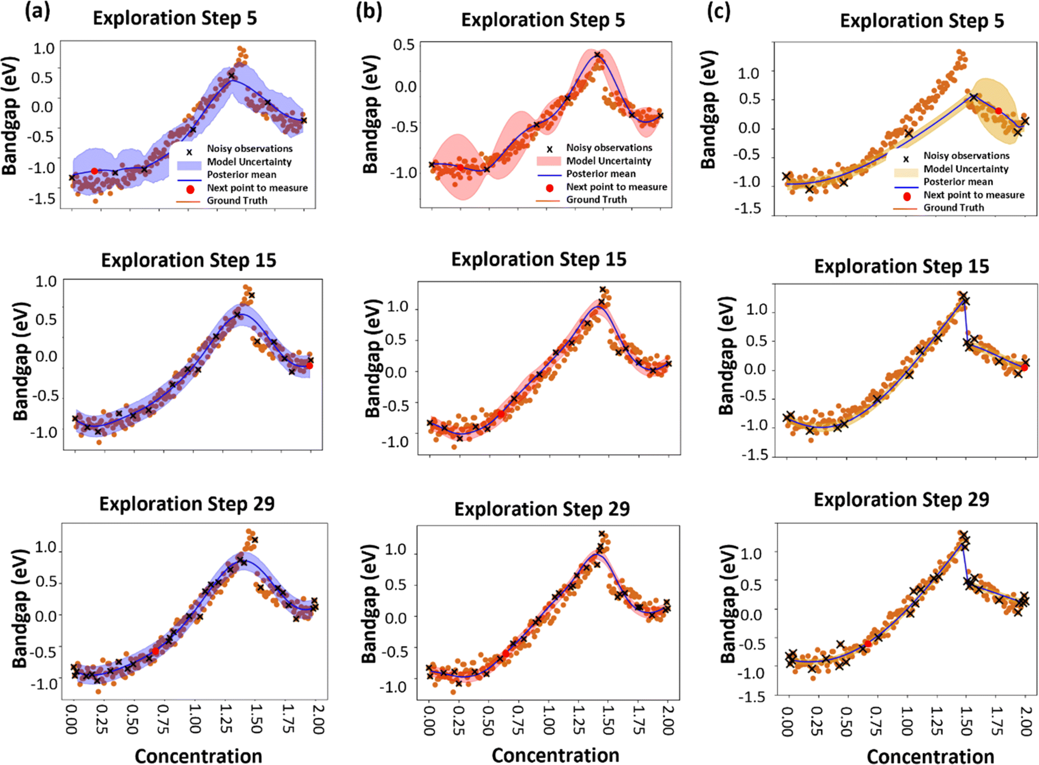Fig. 3 (a) GP model, (b) d-sGP model with a linear mean function, and (c) c-sGP model with a piecewise quadratic mean function for a piecewise quadratic toy model across 30 exploration steps with noise level (0.1) and noise prior (0.01). The figures illustrate the relationship between compositional changes (concentration of GAPbBr₃) and bandgap values. As exploration steps progress, the uncertainty in bandgap predictions decreases significantly, with the c-sGP model showing the most rapid convergence and lowest final uncertainty. Each step demonstrates the model's iterative improvement as more compositional data are incorporated.

The GP model (Fig. 3a) commences with an elevated level of uncertainty, and with each exploration step, the uncertainty gradually decreases, albeit at a slower pace compared to the d-sGP and c-sGP models. Throughout the exploration process, the GP model has a high uncertainty value around 25 between steps 5 and 25 as shown in Fig. 4a. Conversely, the d-sGP model (Fig. 3b) shows a rapid reduction in uncertainty by step 12, compared to the GP model. By the end of the 30 exploration steps, the d-sGP model has not fully converged to the ground truth but provides valuable insights into it. Given our knowledge of the ground truth, the c-sGP model (Fig. 3c) was able to identify the ground truth before exploration step 15 and achieved uncertainty values around 10 by the end of the 30 steps (Fig. 4a).

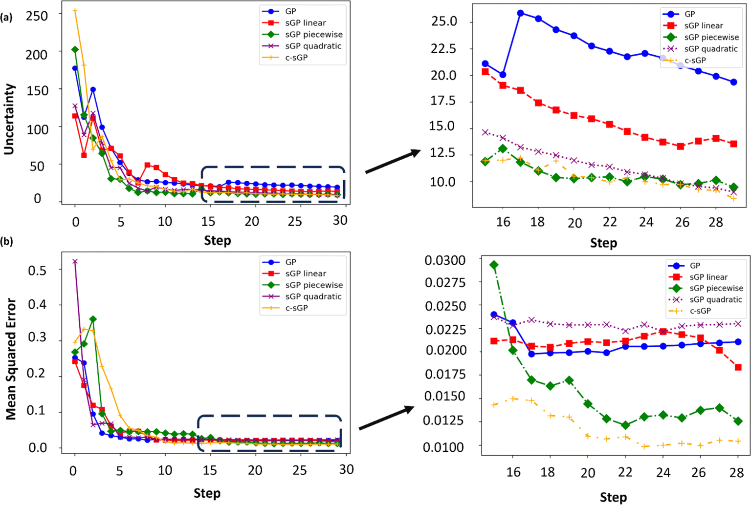Fig. 4 (a) Uncertainty and (b) MSE of piecewise quadratic toy models with comparisons of GP and d-sGP and c-sGP with mean functions linear, quadratic, piecewise and custom piecewise quadratic.

Due to our knowledge of the ground truth, we can also examine the deviation between the predicted posterior mean and the ground truth using the mean squared error (MSE). This allows us to quantify how far off our predictions are from the ground truth. All models in Fig. 4b exhibit low MSE, indicating a close correlation between the predicted posterior mean and the ground truth. Notably, the piecewise mean function shows an increase in correlation between the predicted posterior mean and the ground truth over the exploration steps. The best-performing model is c-sGP, which has the lowest MSE by the end of the 30 exploration steps. This comparison reveals that the c-sGP model demonstrates a more efficient uncertainty reduction process within the given exploration steps. A similar exploration with lower noise (0.01) of the ground truth with a noise prior of (0.1) is shown in Fig. S5.†

Henceforth, we employed the c-sGP methodology to analyze a 1D binary dataset comprising an addition of GAPbBr₃ to MAPbI₃. Our objective was to examine the efficiency of the c-sGP mean function in accurately determining the true nature of this system. Since the ground truth is inaccessible when working with real-world data, we resorted to experimental investigations to elucidate the relationship between the addition of GAPbBr₃ and MAPbI₃. For the custom mean function, bandgap toy models (Fig. S2†) which are based on known bandgap model formations are combined into one custom function. Since the ground truth of our experimental data is unknown and not all defined models may be applicable to the experiment, each bandgap model is given a categorial variable that will represent the ‘weight’ of each model. The weights help decide the influence of each model based on the data. The model with a higher weight will have a higher contribution to the discovery in comparison to the model with a lower weight. The final output will be the average of all the weights. The weights are determined using the Dirichlet distribution which models the probability of k events that are mutually exclusive and collectively exhaustive. This makes it perfect for model mixing occurring in this c-sGP algorithm. To ascertain the mean function exhibiting the least amount of model uncertainty, we conducted a comparative evaluation involving two initial compositions and subsequently expanded the study to encompass a total of thirty compositions (Fig. 5a–c). Similar to GP, d-sGP and c-sGP priors also hold importance in effectively capturing the underlying patterns in the data. To adequately account for the inherent noise in our data, we chose a noise level of 0.01, striking a balance between a low and high noise assumption.

Fig. 5 30-step exploration of bandgap values with varying compositions of GAPbBr₃ added to MAPbI₃. (a) Custom mean function, (b) quadratic mean function, and (c) piecewise mean function. The custom model shows rapid uncertainty reduction within the initial 15 steps, highlighting its adaptability to compositional changes.

In the analysis pertaining to the custom function depicted in Fig. 5a, it is observed that the uncertainty undergoes a rapid reduction within the initial 15 exploratory iterations. During this phase, the uncertainty commences at an amplitude of 270, subsequently declining to approximately 3 by the 15th iteration, as evidenced in Fig. S4.† Contrarily, both the quadratic and piecewise functions, depicted in Fig. 5b and c, continue to manifest pronounced uncertainty magnitudes by the same iteration count. Specifically, the quadratic function initiates with an uncertainty of 5702, reducing to 23 by the aforementioned step, while the piecewise function, beginning at 4720, diminishes to 14. An examination of the scatter plot presented in Fig. S6† indicates superior performance of the c-sGP and Linear d-sGP functions. However, it is imperative to note that the uncertainty inherent to the models should not be the sole criterion for model efficacy; the observations derived from exploratory iterations are equally important. The experimental model exhibits non-linear characteristics, marked by sporadic escalations in bandgaps within specific GAPbBr₃ inclusion ranges, such as sub-20% and interstitially between 50 and 60%. The d-sGP and c-sGP models, interestingly, do not capture all data points pertaining to the measured bandgaps. This deviation may be attributed to the algorithm's tendency to classify certain variations as noise, particularly when data points diverge from the predominant trend exhibited by other points within the dataset.

During the experiment, sGP actively selects the concentration for tests to optimize the mean functions regarding the bandgap model. A set of PL spectra is collected in this process to calculate the bandgap. Notably, spectrum data encompass a variety of physical properties, e.g., various physical properties other than bandgaps are encompassed in the PL spectrum. The influence exerted by the addition of GAPbBr₃ can be readily seen through the discernible augmentation of raw spectral data. Our previous work also demonstrated that additional insights can be gained through counterfactual analysis of the dataset acquired via GP active learning driven experiments.⁶⁰ Therefore, here we performed additional analyses of raw PL spectra and absorbance to get a deeper understanding of the material system. Notably, there is an increase in intensity with low addition of GAPbBr₃ (2 to 6%) as shown in Fig. S7b† where the PL peak doesn't have an obvious shift. This may be attributed to the passivation action of GAPbBr₃ towards the defect at the MAPbI₃ surface; here the ions are not permeated towards the bulk perovskite lattice.⁶¹ However, a change in this observed trend becomes apparent upon further increments in the concentration of GAPbBr₃, wherein the PL experiences a blue-shift and a concurrent decrease in intensity up to 80% (Fig. 6a and S7a†). The origin of this peak shift may be due to bandgap variation due to halide substitution. MAPbI₃ has a lower bandgap, which has a PL peak around the 750 nm region. On the other hand, GAPbBr₃, being bromide-based, has a higher bandgap which translates to a PL peak in the blue-region. This leads to a gradual blue shift of the PL peak.^43,62 This decrease in intensity can possibly be attributed to various reasons such as the crystal structure evolution where the mixed-halide system can have halide rich regions that can create non-radiative recombination pathways.^63,64 Also as the bromide content increases, the bandgap widens which can impact the PL intensity.^24,62 Moreover, a distinct alteration in the absorption spectrum is observed with the introduction of GAPbBr₃. Specifically, the characteristic absorbance peak, localized around 800 nm, vanishes as the concentration of GAPbBr₃ increases, being replaced by new peaks that manifest in the range of 640 nm to 550 nm when approximately 50% of GAPbBr₃ is introduced (Fig. 6b).

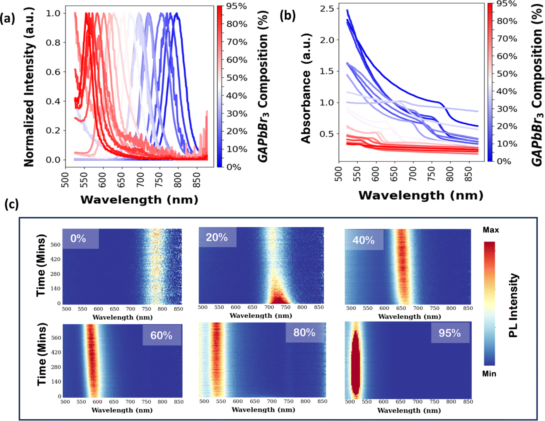Fig. 6 The experimental data for 20 mixed MAPbI₃ and GAPbBr₃ with various concentrations. (a) Normalized PL spectra, (b) absorbance spectra and (c) time dependent photoluminescence spectra heatmaps with various additions of GAPbBr₃ to MAPbI₃.

c-sGP's performance, as seen in Fig. 5a, shows that the c-sGP model captures the non-linear characteristics of the bandgap changes, including the jumps corresponding to possible differing phases. These jumps are consistent with the PL data and absorbance data shown in Fig. 6.

To provide further structural analysis, X-ray Diffraction (XRD) was performed on four samples of the GAPbBr₃–MAPbI₃ mixture (Fig. 7). With increasing GA content, we made 0%, 20%, 65%, and 95% thin films. The XRD analysis revealed key structural transformations within the perovskite material as the concentration of GAPbBr₃ increased. Notably, there is evidence of phase segregation and the formation of secondary phases at higher concentrations, manifesting as shifts in the diffraction peaks and the emergence of new peaks. In our XRD pattern for pure MAPbI₃, we see characteristic peaks of the tetragonal phase at 2θ = 14.5° and 28.7° corresponding to the (1 1 0) and (2 2 0) planes.⁶⁵ As the amount of GAPbBr₃ is added into MAPbI₃ there is an observed shift in the diffraction peaks towards lower angles. This is due to the influence of the GA cation. There is an indication of an expansion of the unit cell due to the large GA cation (ionic radius = 278 pm)⁴¹ substituting the MA cation (ionic radius = 217 pm).⁴⁵ This is in correlation with Fig. 6(a) where we see a blue shift of the PL as the concentration of GAPbBr₃ increases which is indicative of an increasing bandgap.

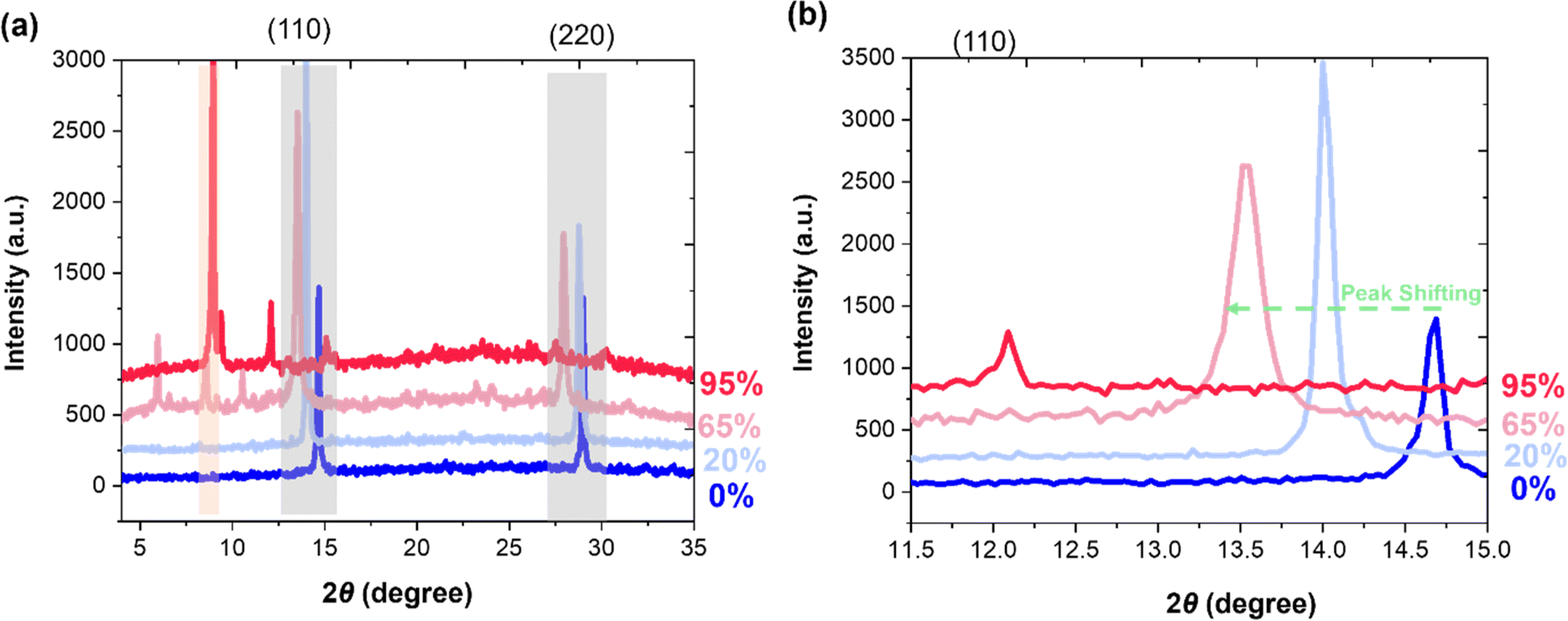Fig. 7 (a) XRD spectra of MAGAPb (BrI)₃ with increasing GA content, and (b) zoom-in spectra of the (110) plane.

A tolerance factor in the range 0.8–1.0 results in the formation of a three-dimensional (3D) cubic perovskite structure.⁶⁶ MAPbI₃ has a tolerance factor of ∼0.8, while that of GAPbBr₃ is calculated to be ∼1.4.⁶⁷ This suggests that pure GA lead bromide crystallizes in a lower-dimensional perovskite structure. In addition to the tolerance factor, the octahedral factor (μ) is also relevant for the formation of the perovskite structure. The octahedral factor (μ) is the ratio between the ionic radii of B and X ions. In our case, when the I⁻ (r_avg ∼ 198 pm) is replaced by the Br⁻ ion (r_avg ∼ 185 pm), which is smaller than I⁻, it results in an increase of the octahedral factor.⁶⁷ However, this also implies that the decrease in the halogen ion size reduces the BX₆ octahedral size accommodating the larger GA cation in the MAPbI₃ lattice.

When the GABr concentration is increased from 1 to 20%, the larger GA cation can substitute for MA only within a limit governed by the tolerance and octahedral factors. This is evident from the low angle shift of the XRD peaks suggesting an expansion of the unit cell due to the larger GA cation (Fig. 7b). We observe that once the GABr concentration crosses a certain limit ∼65%, there is emergence of additional peaks in the diffraction pattern indicating other phases in the film as the MAPbI₃ lattice can no longer accommodate the GA cations at such high concentrations. This is also supported by the diminishing of the peaks in the 20–30° 2θ range. Further increasing the concentration increases the formation of GA lead halide phases. The XRD pattern of the 95% GAMA matches with GAPbBr₃ confirming the formation of a complete GA cation based two-dimensional (2D) perovskite.

Yet, phase segregation is not observed in the time-dependent PL, which was measured over a continuous duration of 12 hours under ambient conditions as depicted in Fig. 6c. The PL over time was shown for 0, 20, 40, 60, 80, and 95%. We can see that over time the intensity of pure MAPbI₃ remains the same without any PL peak shifts. As we add a higher amount of GAPbBr₃, there is evidence of blue shifting over time for 20% addition, and at 40% over the 12 hours, there are no apparent PL peak shifts, and the intensity remains high for the total time. We see a systematic shift in the PL peak as we continue to add GAPbBr₃ with an increase in PL intensity. Given that we have observed PL peaks above 550 nm in our GA-rich cases (Br-rich system) and that there is no nominal absorption band-edge with no appreciable excitonic peak, the 2D phase of GABr has not been formed. The use of GA ions has been reported to passivate defects in the perovskite systems, which can reduce non-radiative recombinations.^41,43,68 The steric suppression of phase segregation can stabilize the bandgap under illumination,⁶⁹ which is an indicator that the phase separation observed in the XRD results does not impact the bandgap model in a mixed GA and MA system. GA can serve as a modifying agent within the perovskite structure by influencing phase stability and ion migration by various mechanisms. First, GA ions due to their larger cation size can distort the perovskite lattice, reducing the tendency for phase segregation. Regions where the GA ion is too large to fit neatly within the lattice can also create voids or gaps. These gaps can act as barriers to ion migration, effectively pinning the ions in place and stabilizing the material. Moreover, the c-sGP model shows intervals of bandgap fluctuations interstitially between 50 and 60% addition of GAPbBr₃. This suggests that the mean function in sGP can provide insights into structural changes. The machine learning model aims to account for the ‘apparent’ bandgap based on the designed composition ratio. Even if there may be some secondary phases in the film, the machine learning model accounts for noise in the system, meaning it can still uncover the underlying bandgap model.

The ensuing thin film observations, as depicted in Fig. S5c,† show that pure MAPbI₃ films have a medium brown color. When a low amount of GAPbBr₃ (below 12%) is added the color of the films turns deep brown, then a lighter brown color at higher quantities of GAPbBr₃. Addition of GAPbBr₃ has also been shown to increase the intensity of the PL in tandem with a small addition of GAPbBr₃ (as observed in Fig. S7b†). It is evident that concentrations below the 20% threshold exhibit minimal alterations in the quantified bandgap, no halide segregation or phase transition and seemly increase the PL intensity. At 20% the bandgap has increased from 1.604 eV to 1.703 eV (Fig. S8†) and remains around 1.7 eV up to 40%. After this addition percentage the bandgap jumps up to 2.0 eV and remains around there with increasing addition of GAPbBr₃.

In comparison, phase segregation in mixed halide perovskites, such as in MAPbI₃ and MAPbBr₃, becomes particularly pronounced when exposed to ambient conditions.^63,70,71 Under environmental influences such as light^9,64,70 and moisture,^71,72 the mixed halide perovskite tends to separate into its individual components. Phase segregation can induce localized regions of iodide-rich or bromide-rich domains. This process will reduce the overall homogeneity of the mixed material and can compromise its optoelectronic properties. Incorporating GA into the A-site cation in MA-based hybrid perovskite has led to enhanced stability and even better air stability than MAPbI₃.⁷³

The blending of mixed halide perovskite materials tends to result in bandgap behavior that is characterized by different models based on the specific components being mixed. For example, mixing halides such as iodide, bromide and chloride tend to result in a linear model,^24,74 whereas, mixing divalent cations such as lead and tin exhibits a bowing model.^75–77 In this case, we see some apparent jumps or anomalies in the bandgap, especially above 40% addition of GAPbBr₃ which can possibly be influenced by certain factors, such as, GA being large enough that it can't exactly occupy the A-site cation between the [PbI₆]⁴⁻ arrays, causing induced local lattice distortions.^41,78 Also, pure GAPbBr₃ doesn't exist in a 3D phase, and the introduction of GAPbBr₃ into MAPbI₃ may induce some structural changes or phase transitions leading to this variation in the bandgap.⁷⁹ Overall, utilizing sGP allows us to not only identify some underlying physical models, but also pinpoint areas for optimization. The ability to discern intricate relationships and its capability to parse complex material datasets shows its power in material discovery and optimization.

In this study, we have successfully applied the workflow to the sequential process of thin film preparation. This methodology can easily be extended to accommodate automated synthesis workflows such as microfluidics, pipetting robots,^80–86 and fully autonomous labs. Incorporation of higher dimensional spaces and implementing batch updates allows this workflow to be adaptable to a broader range of experimental scenarios. To expedite BO and facilitate the simultaneous discovery of the physical model, we have developed a novel algorithm. This algorithm offers a significant acceleration in the optimization process, allowing for more efficient exploration and exploitation of the parameter space. The mean function, which is a principal component of our algorithm, embodies the physical behaviors and characteristics of the system by capturing the essential features and potential mechanisms that drive discovery and material optimization during the active experiment. This joint exploration of the parameter space and active discovery of the physical model contributes to the advancement of scientific understanding and optimization of material properties. Overall, our approach demonstrates the effectiveness of incorporating the mean function, which encapsulates the physical behaviors of the system. This integration enhances the efficiency of the optimization process, facilitating more effective and targeted experiments for the discovery and optimization of materials.

Data availability

The code for structured gaussian processing (sGP) can be found at https://github.com/SLKS99/-Physics-driven-discovery-and-optimization-of-hybrid-perovskite-films. The data and machine learning method are both available in the github link.

Conflicts of interest

There are no conflicts to declare.

Acknowledgements

S. S., E. F., J. Y. and M. A. acknowledge support from the National Science Foundation (NSF), award number 2043205. The authors acknowledge support from the Center for Nanophase Materials Sciences (CNMS) user facility, project CNMS2023-A-01927, which is a US Department of Energy, Office of Science User Facility at Oak Ridge National Laboratory. S. S. acknowledges the support from the Center of Materials Processing (CMP), a Tennessee Higher Education Commission (THEC) supported Accomplished Center of Excellence.

References

1. A. Kojima, K. Teshima, Y. Shirai and T. Miyasaka, Organometal Halide Perovskites as Visible-Light Sensitizers for Photovoltaic Cells, J. Am. Chem. Soc., 2009, 131(17), 6050–6051,  DOI:10.1021/ja809598r.
2. J. Park, J. Kim, H.-S. Yun, M. J. Paik, E. Noh, H. J. Mun, M. G. Kim, T. J. Shin and S. I. Seok, Controlled growth of perovskite layers with volatile alkylammonium chlorides, Nature, 2023, 616(7958), 724–730,  DOI:10.1038/s41586-023-05825-y.
3. S. Mariotti, E. Köhnen, F. Scheler, K. Sveinbjörnsson, L. Zimmermann, M. Piot, F. Yang, B. Li, J. Warby and A. Musiienko, et al., Interface engineering for high-performance, triple-halide perovskite–silicon tandem solar cells, Science, 2023, 381(6653), 63–69,  DOI:10.1126/science.adf5872.
4. P. K. Kung, M. H. Li, P. Y. Lin, Y. H. Chiang, C. R. Chan, T. F. Guo and P. Chen, A review of inorganic hole transport materials for perovskite solar cells, Adv. Mater. Interfaces, 2018, 5(22), 1800882.
5. D. J. Kubicki, D. Prochowicz, A. Hofstetter, M. Saski, P. Yadav, D. Bi, N. Pellet, J. Lewinski, S. M. Zakeeruddin, M. Gratzel and L. Emsley, Formation of Stable Mixed Guanidinium-Methylammonium Phases with Exceptionally Long Carrier Lifetimes for High-Efficiency Lead Iodide-Based Perovskite Photovoltaics, J. Am. Chem. Soc., 2018, 140(9), 3345–3351,  DOI:10.1021/jacs.7b12860.
6. J. He, W.-H. Fang, R. Long and O. V. Prezhdo, Increased Lattice Stiffness Suppresses Nonradiative Charge Recombination in MAPbI₃ Doped with Larger Cations: Time-Domain Ab Initio Analysis, ACS Energy Lett., 2018, 3(9), 2070–2076,  DOI:10.1021/acsenergylett.8b01191.
7. N. D. Pham, C. Zhang, V. T. Tiong, S. Zhang, G. Will, A. Bou, J. Bisquert, P. E. Shaw, A. Du, G. J. Wilson and H. Wang, Tailoring Crystal Structure of FA0.83Cs0.17PbI₃ Perovskite Through Guanidinium Doping for Enhanced Performance and Tunable Hysteresis of Planar Perovskite Solar Cells, Adv. Funct. Mater., 2019, 29(1), 1806479,  DOI:10.1002/adfm.201806479.
8. W. Yang, H. Long, X. Sha, J. Sun, Y. Zhao, C. Guo, X. Peng, C. Shou, X. Yang and J. Sheng, et al., Unlocking Voltage Potentials of Mixed-Halide Perovskite Solar Cells via Phase Segregation Suppression, Adv. Funct. Mater., 2022, 32(12), 2110698,  DOI:10.1002/adfm.202110698.
9. K. Datta, B. T. van Gorkom, Z. Chen, M. J. Dyson, T. P. A. van der Pol, S. C. J. Meskers, S. Tao, P. A. Bobbert, M. M. Wienk and R. A. J. Janssen, Effect of Light-Induced Halide Segregation on the Performance of Mixed-Halide Perovskite Solar Cells, ACS Appl. Energy Mater., 2021, 4(7), 6650–6658,  DOI:10.1021/acsaem.1c00707.
10. E. T. Hoke, D. J. Slotcavage, E. R. Dohner, A. R. Bowring, H. I. Karunadasa and M. D. McGehee, Reversible photo-induced trap formation in mixed-halide hybrid perovskites for photovoltaics, Chem. Sci., 2015, 6(1), 613–617,  10.1039/C4SC03141E.
11. Y. Liu, M. Wang, A. V. Ievlev, A. Ahmadi, J. K. Keum, M. Ahmadi, B. Hu and O. S. Ovchinnikova, Photoinduced iodide repulsion and halides-demixing in layered perovskites, Mater. Today Nano, 2022, 18, 100197,  DOI:10.1016/j.mtnano.2022.100197.
12. S. Adjokatse, H.-H. Fang and M. A. Loi, Broadly tunable metal halide perovskites for solid-state light-emission applications, Mater. Today, 2017, 20(8), 413–424,  DOI:10.1016/j.mattod.2017.03.021.
13. D. B. Straus and R. J. Cava, Tuning the Band Gap in the Halide Perovskite CsPbBr₃ through Sr Substitution, ACS Appl. Mater. Interfaces, 2022, 14(30), 34884–34890,  DOI:10.1021/acsami.2c09275.
14. Y. Hassan, J. H. Park, M. L. Crawford, A. Sadhanala, J. Lee, J. C. Sadighian, E. Mosconi, R. Shivanna, E. Radicchi and M. Jeong, et al., Ligand-engineered bandgap stability in mixed-halide perovskite LEDs, Nature, 2021, 591(7848), 72–77,  DOI:10.1038/s41586-021-03217-8.
15. C. W. Ahn, J. H. Jo, J. S. Choi, Y. H. Hwang, I. W. Kim and T. H. Kim, Heteroanionic Lead-Free Double-Perovskite Halides for Bandgap Engineering, Adv. Eng. Mater., 2023, 25(1), 2201119,  DOI:10.1002/adem.202201119.
16. J. Wen, Y. Zhao, Z. Liu, H. Gao, R. Lin, S. Wan, C. Ji, K. Xiao, Y. Gao and Y. Tian, et al., Steric Engineering Enables Efficient and Photostable Wide-Bandgap Perovskites for All-Perovskite Tandem Solar Cells, Adv. Mater., 2022, 34(26), 2110356,  DOI:10.1002/adma.202110356.
17. M. M. Byranvand, C. Otero-Martínez, J. Ye, W. Zuo, L. Manna, M. Saliba, R. L. Z. Hoye and L. Polavarapu, Recent Progress in Mixed A-Site Cation Halide Perovskite Thin-Films and Nanocrystals for Solar Cells and Light-Emitting Diodes, Adv. Opt. Mater., 2022, 10(14), 2200423,  DOI:10.1002/adom.202200423.
18. G. Kim, H. Min, K. S. Lee, D. Y. Lee, S. M. Yoon and S. I. Seok, Impact of strain relaxation on performance of α-formamidinium lead iodide perovskite solar cells, Science, 2020, 370(6512), 108–112,  DOI:10.1126/science.abc4417.
19. T. Duong, T. Nguyen, K. Huang, H. Pham, S. G. Adhikari, M. R. Khan, L. Duan, W. Liang, K. C. Fong and H. Shen, et al., Bulk Incorporation with 4-Methylphenethylammonium Chloride for Efficient and Stable Methylammonium-Free Perovskite and Perovskite-Silicon Tandem Solar Cells, Adv. Energy Mater., 2023, 13(9), 2203607,  DOI:10.1002/aenm.202203607.
20. H. Wang, H. Liu, Z. Dong, W. Li, L. Zhu and H. Chen, Composition manipulation boosts the efficiency of carbon-based CsPbI3 perovskite solar cells to beyond 14%, Nano Energy, 2021, 84, 105881,  DOI:10.1016/j.nanoen.2021.105881.
21. J.-W. Lee, S. Tan, S. I. Seok, Y. Yang and N.-G. Park, Rethinking the A cation in halide perovskites, Science, 2022, 375(6583), eabj1186,  DOI:10.1126/science.abj1186.
22. A. Amat, E. Mosconi, E. Ronca, C. Quarti, P. Umari, M. K. Nazeeruddin, M. Grätzel and F. De Angelis, Cation-Induced Band-Gap Tuning in Organohalide Perovskites: Interplay of Spin–Orbit Coupling and Octahedra Tilting, Nano Lett., 2014, 14(6), 3608–3616,  DOI:10.1021/nl5012992.
23. K. Higgins, S. M. Valleti, M. Ziatdinov, S. V. Kalinin and M. Ahmadi, Chemical Robotics Enabled Exploration of Stability in Multicomponent Lead Halide Perovskites via Machine Learning, ACS Energy Lett., 2020, 5(11), 3426–3436,  DOI:10.1021/acsenergylett.0c01749.
24. J. H. Noh, S. H. Im, J. H. Heo, T. N. Mandal and S. I. Seok, Chemical Management for Colorful, Efficient, and Stable Inorganic–Organic Hybrid Nanostructured Solar Cells, Nano Lett., 2013, 13(4), 1764–1769,  DOI:10.1021/nl400349b.
25. C. M. Sutter-Fella, Y. Li, M. Amani, J. W. Ager III, F. M. Toma, E. Yablonovitch, I. D. Sharp and A. Javey, High Photoluminescence Quantum Yield in Band Gap Tunable Bromide Containing Mixed Halide Perovskites, Nano Lett., 2016, 16(1), 800–806,  DOI:10.1021/acs.nanolett.5b04884.
26. M. Green, E. Dunlop, J. Hohl-Ebinger, M. Yoshita, N. Kopidakis and X. Hao, Solar cell efficiency tables (version 57), Prog. Photovoltaics, 2020, 29(1), 3–15,  DOI:10.1002/pip.3371.
27. K. Suchan, J. Just, P. Beblo, C. Rehermann, A. Merdasa, R. Mainz, I. G. Scheblykin and E. Unger, Multi-Stage Phase-Segregation of Mixed Halide Perovskites under Illumination: A Quantitative Comparison of Experimental Observations and Thermodynamic Models, Adv. Funct. Mater., 2023, 33(3), 2206047,  DOI:10.1002/adfm.202206047.
28. S. Kahmann, Z. Chen, O. Hordiichuk, O. Nazarenko, S. Shao, M. V. Kovalenko, G. R. Blake, S. Tao and M. A. Loi, Compositional Variation in FAPb_(1−x)Sn_(x)I₍₃₎ and Its Impact on the Electronic Structure: A Combined Density Functional Theory and Experimental Study, ACS Appl. Mater. Interfaces, 2022, 14(30), 34253–34261,  DOI:10.1021/acsami.2c00889.
29. A. Goyal, S. McKechnie, D. Pashov, W. Tumas, M. van Schilfgaarde and V. Stevanović, Origin of Pronounced Nonlinear Band Gap Behavior in Lead–Tin Hybrid Perovskite Alloys, Chem. Mater., 2018, 30(11), 3920–3928,  DOI:10.1021/acs.chemmater.8b01695.
30. P. F. Ndione, Z. Li and K. Zhu, Effects of alloying on the optical properties of organic–inorganic lead halide perovskite thin films, J. Mater. Chem. C, 2016, 4(33), 7775–7782,  10.1039/C6TC02135B.
31. S. Tao, I. Schmidt, G. Brocks, J. Jiang, I. Tranca, K. Meerholz and S. Olthof, Absolute energy level positions in tin- and lead-based halide perovskites, Nat. Commun., 2019, 10(1), 2560,  DOI:10.1038/s41467-019-10468-7.
32. S. Olthof, Research Update: The electronic structure of hybrid perovskite layers and their energetic alignment in devices, APL Mater., 2016, 4(9) DOI:10.1063/1.4960112.
33. J. Emara, T. Schnier, N. Pourdavoud, T. Riedl, K. Meerholz and S. Olthof, Impact of Film Stoichiometry on the Ionization Energy and Electronic Structure of CH₃NH₃PbI₃ Perovskites, Adv. Mater., 2016, 28(3), 553–559,  DOI:10.1002/adma.201503406.
34. Y. Yin, Y. Wang, Q. Sun, Y. Yang, Y. Wang, Z. Yang and W. J. Yin, Unique Photoelectric Properties and Defect Tolerance of Lead-Free Perovskite Cs₍₃₎Cu₍₂₎I₍₅₎ with Highly Efficient Blue Emission, J. Phys. Chem. Lett., 2022, 13(18), 4177–4183,  DOI:10.1021/acs.jpclett.2c00888.
35. B. Subedi, C. Li, C. Chen, D. Liu, M. M. Junda, Z. Song, Y. Yan and N. J. Podraza, Urbach Energy and Open-Circuit Voltage Deficit for Mixed Anion–Cation Perovskite Solar Cells, ACS Appl. Mater. Interfaces, 2022, 14(6), 7796–7804,  DOI:10.1021/acsami.1c19122.
36. P. Basumatary, J. Kumari and P. Agarwal, Probing the defects states in MAPbI3 perovskite thin films through photoluminescence and photoluminescence excitation spectroscopy studies, Optik, 2022, 266 DOI:10.1016/j.ijleo.2022.169586.
37. Y. Liu, A. V. Ievlev, N. Borodinov, M. Lorenz, K. Xiao, M. Ahmadi, B. Hu, S. V. Kalinin and O. S. Ovchinnikova, Direct Observation of Photoinduced Ion Migration in Lead Halide Perovskites, Adv. Funct. Mater., 2020, 31(8) DOI:10.1002/adfm.202008777.
38. Y. Liu, N. Borodinov, M. Lorenz, M. Ahmadi, S. V. Kalinin, A. V. Ievlev and O. S. Ovchinnikova, Hysteretic Ion Migration and Remanent Field in Metal Halide Perovskites, Adv. Sci., 2020, 7(19), 2001176,  DOI:10.1002/advs.202001176.
39. A. Mahapatra, R. Runjhun, J. Nawrocki, J. Lewiński, A. Kalam, P. Kumar, S. Trivedi, M. M. Tavakoli, D. Prochowicz and P. Yadav, Elucidation of the role of guanidinium incorporation in single-crystalline MAPbI₃ perovskite on ion migration and activation energy, Phys. Chem. Chem. Phys., 2020, 22(20), 11467–11473,  10.1039/D0CP01119C.
40. D. J. Kubicki, D. Prochowicz, A. Hofstetter, M. Saski, P. Yadav, D. Bi, N. Pellet, J. Lewiński, S. M. Zakeeruddin, M. Grätzel and L. Emsley, Formation of Stable Mixed Guanidinium–Methylammonium Phases with Exceptionally Long Carrier Lifetimes for High-Efficiency Lead Iodide-Based Perovskite Photovoltaics, J. Am. Chem. Soc., 2018, 140(9), 3345–3351,  DOI:10.1021/jacs.7b12860.
41. A. D. Jodlowski, C. Roldán-Carmona, G. Grancini, M. Salado, M. Ralaiarisoa, S. Ahmad, N. Koch, L. Camacho, G. De Miguel and M. K. Nazeeruddin, Large guanidinium cation mixed with methylammonium in lead iodide perovskites for 19% efficient solar cells, Nat. Energy, 2017, 2(12), 972–979.
42. P. P. Boix, S. Agarwala, T. M. Koh, N. Mathews and S. G. Mhaisalkar, Perovskite Solar Cells: Beyond Methylammonium Lead Iodide, J. Phys. Chem. Lett., 2015, 6(5), 898–907,  DOI:10.1021/jz502547f.
43. M. Balaji Gandhi, A. Valluvar Oli, S. Nicholson, M. Adelt, R. Martin, Y. Chen, M. Babu Sridharan and A. Ivaturi, Investigation on guanidinium bromide incorporation in methylammonium lead iodide for enhanced efficiency and stability of perovskite solar cells, Sol. Energy, 2023, 253, 1–8,  DOI:10.1016/j.solener.2023.01.026.
44. M. A. Ziatdinov, A. Ghosh and S. V. Kalinin, Physics makes the difference: Bayesian optimization and active learning via augmented Gaussian process, Mach. Learn., 2022, 3(1), 015003,  DOI:10.1088/2632-2153/ac4baa.
45. W. Zhang, J. Xiong, J. Li and W. A. Daoud, Guanidinium induced phase separated perovskite layer for efficient and highly stable solar cells, J. Mater. Chem. A, 2019, 7(16), 9486–9496.
46. C. E. Rasmussen and C. K. I. Williams, Gaussian Processes for Machine Learning (Adaptive Computation and Machine Learning), The MIT Press, 2005.
47. B. Lambert, A Student's Guide to Bayesian Statistics, SAGE Publications Ltd, 1st edn, 2018.
48. O. Martin, Bayesian Analysis with Python: Introduction to statistical modeling and probabilistic programming using PyMC3 and ArviZ, Packt Publishing, 2nd edn, 2018.
49. R. Garnett, Bayesian Optimization, Cambridge University Press, 2022, https://bayesoptbook.com.
50. M. M. Noack, G. S. Doerk, R. Li, J. K. Streit, R. A. Vaia, K. G. Yager and M. Fukuto, Autonomous materials discovery driven by Gaussian process regression with inhomogeneous measurement noise and anisotropic kernels, Sci. Rep., 2020, 10(1), 17663,  DOI:10.1038/s41598-020-74394-1.
51. M. Ahmadi, M. Ziatdinov, Y. Zhou, E. A. Lass and S. V. Kalinin, Machine learning for high-throughput experimental exploration of metal halide perovskites, Joule, 2021, 5(11), 2797–2822,  DOI:10.1016/j.joule.2021.10.001.
52. S. Ament, M. Amsler, D. R. Sutherland, M.-C. Chang, D. Guevarra, A. B. Connolly, J. M. Gregoire, M. O. Thompson, C. P. Gomes and R. B. van Dover, Autonomous materials synthesis via hierarchical active learning of nonequilibrium phase diagrams, Sci. Adv., 2021, 7(51), eabg4930,  DOI:10.1126/sciadv.abg4930.
53. M. Ziatdinov, Y. Liu, K. Kelley, R. Vasudevan and S. V. Kalinin, Bayesian Active Learning for Scanning Probe Microscopy: From Gaussian Processes to Hypothesis Learning, ACS Nano, 2022, 16(9), 13492–13512,  DOI:10.1021/acsnano.2c05303.
54. Y. Liu, J. Yang, R. K. Vasudevan, K. P. Kelley, M. Ziatdinov, S. V. Kalinin and M. Ahmadi, Exploring the Relationship of Microstructure and Conductivity in Metal Halide Perovskites via Active Learning-Driven Automated Scanning Probe Microscopy, J. Phys. Chem. Lett., 2023, 14(13), 3352–3359,  DOI:10.1021/acs.jpclett.3c00223.
55. Y. Liu, K. P. Kelley, R. K. Vasudevan, H. Funakubo, M. A. Ziatdinov and S. V. Kalinin, Experimental discovery of structure–property relationships in ferroelectric materials via active learning, Nat. Mach. Intell., 2022, 4(4), 341–350,  DOI:10.1038/s42256-022-00460-0.
56. J. Boelrijk, B. Pirok, B. Ensing and P. Forré, Bayesian optimization of comprehensive two-dimensional liquid chromatography separations, J. Chromatogr. A, 2021, 1659, 462628,  DOI:10.1016/j.chroma.2021.462628.
57. J. Boelrijk, B. Ensing, P. Forré and B. W. J. Pirok, Closed-loop automatic gradient design for liquid chromatography using Bayesian optimization, Anal. Chim. Acta, 2023, 1242, 340789,  DOI:10.1016/j.aca.2023.340789.
58. S. Stanton, W. Maddox, N. Gruver, P. Maffettone, E. Delaney, P. Greenside and A. G. Wilson, Accelerating Bayesian Optimization for Biological Sequence Design with Denoising Autoencoders, in Proceedings of the 39th International Conference on Machine Learning, Proceedings of Machine Learning Research, 2022.
59. M. A. Ziatdinov, Y. Liu, A. N. Morozovska, E. A. Eliseev, X. Zhang, I. Takeuchi and S. V. Kalinin, Hypothesis Learning in Automated Experiment: Application to Combinatorial Materials Libraries, Adv. Mater., 2022, 34(20), 2201345,  DOI:10.1002/adma.202201345.
60. Y. Liu, A. N. Morozovska, E. A. Eliseev, K. P. Kelley, R. Vasudevan, M. Ziatdinov and S. V. Kalinin, Autonomous scanning probe microscopy with hypothesis learning: Exploring the physics of domain switching in ferroelectric materials, Patterns, 2023, 4(3), 100704,  DOI:10.1016/j.patter.2023.100704.
61. W. H. Jeong, Z. Yu, L. Gregori, J. Yang, S. R. Ha, J. W. Jang, H. Song, J. H. Park, E. D. Jung and M. H. Song, et al., In situ cadmium surface passivation of perovskite nanocrystals for blue LEDs, J. Mater. Chem. A, 2021, 9(47), 26750–26757,  10.1039/D1TA08756H.
62. S. A. Kulkarni, T. Baikie, P. P. Boix, N. Yantara, N. Mathews and S. Mhaisalkar, Band-gap tuning of lead halide perovskites using a sequential deposition process, J. Mater. Chem. A, 2014, 2(24), 9221–9225,  10.1039/C4TA00435C.
63. A. J. Knight, J. Borchert, R. D. J. Oliver, J. B. Patel, P. G. Radaelli, H. J. Snaith, M. B. Johnston and L. M. Herz, Halide Segregation in Mixed-Halide Perovskites: Influence of A-Site Cations, ACS Energy Lett., 2021, 6(2), 799–808,  DOI:10.1021/acsenergylett.0c02475.
64. M. C. Brennan, S. Draguta, P. V. Kamat and M. Kuno, Light-Induced Anion Phase Segregation in Mixed Halide Perovskites, ACS Energy Lett., 2018, 3(1), 204–213,  DOI:10.1021/acsenergylett.7b01151.
65. Y. Zhao and K. Zhu, Charge transport and recombination in perovskite (CH₃NH₃) PbI₃ sensitized TiO₂ solar cells, J. Phys. Chem. Lett., 2013, 4(17), 2880–2884.
66. M. R. Filip and F. Giustino, The geometric blueprint of perovskites, Proc. Natl. Acad. Sci. U. S. A., 2018, 115(21), 5397–5402.
67. M. B. Gandhi, A. V. Oli, S. Nicholson, M. Adelt, R. Martin, Y. Chen, M. B. Sridharan and A. Ivaturi, Investigation on guanidinium bromide incorporation in methylammonium lead iodide for enhanced efficiency and stability of perovskite solar cells, Sol. Energy, 2023, 253, 1–8.
68. M. Guan, P. Li, Y. Wu, X. Liu, S. Xu and J. Zhang, Highly efficient green emission Cs₄PbBr₆ quantum dots with stable water endurance, Opt. Lett., 2022, 47(19), 5020–5023,  DOI:10.1364/OL.471088.
69. L. Grater, M. Wang, S. Teale, S. Mahesh, A. Maxwell, Y. Liu, S. M. Park, B. Chen, F. Laquai, M. G. Kanatzidis and E. H. Sargent, Sterically Suppressed Phase Segregation in 3D Hollow Mixed-Halide Wide Band Gap Perovskites, J. Phys. Chem. Lett., 2023, 14(26), 6157–6162,  DOI:10.1021/acs.jpclett.3c01156.
70. R. A. Kerner, Z. Xu, B. W. Larson and B. P. Rand, The role of halide oxidation in perovskite halide phase separation, Joule, 2021, 5(9), 2273–2295,  DOI:10.1016/j.joule.2021.07.011.
71. A. J. Knight, A. D. Wright, J. B. Patel, D. P. McMeekin, H. J. Snaith, M. B. Johnston and L. M. Herz, Electronic Traps and Phase Segregation in Lead Mixed-Halide Perovskite, ACS Energy Lett., 2019, 4(1), 75–84,  DOI:10.1021/acsenergylett.8b02002.
72. J.-W. Lee, D.-H. Kim, H.-S. Kim, S.-W. Seo, S. M. Cho and N.-G. Park, Formamidinium and Cesium Hybridization for Photo- and Moisture-Stable Perovskite Solar Cell, Adv. Energy Mater., 2015, 5(20), 1501310,  DOI:10.1002/aenm.201501310.
73. Y. Kim, C. Bae, H. S. Jung and H. Shin, Enhanced stability of guanidinium-based organic–inorganic hybrid lead triiodides in resistance switching, APL Mater., 2019, 7(8) DOI:10.1063/1.5109525.
74. D. Cui, Z. Yang, D. Yang, X. Ren, Y. Liu, Q. Wei, H. Fan and J. Zeng, Color-Tuned Perovskite Films Prepared for Efficient Solar Cell Applications, J. Phys. Chem. C, 2015, 120 DOI:10.1021/acs.jpcc.5b09393.
75. K. Galkowski, A. Surrente, M. Baranowski, B. Zhao, Z. Yang, A. Sadhanala, S. Mackowski, S. D. Stranks and P. Plochocka, Excitonic Properties of Low-Band-Gap Lead–Tin Halide Perovskites, ACS Energy Lett., 2019, 4(3), 615–621,  DOI:10.1021/acsenergylett.8b02243.
76. A. Rajagopal, R. J. Stoddard, H. W. Hillhouse and A. K. Y. Jen, On understanding bandgap bowing and optoelectronic quality in Pb–Sn alloy hybrid perovskites, J. Mater. Chem. A, 2019, 7(27), 16285–16293,  10.1039/C9TA05308E.
77. F. Hao, C. C. Stoumpos, R. P. H. Chang and M. G. Kanatzidis, Anomalous Band Gap Behavior in Mixed Sn and Pb Perovskites Enables Broadening of Absorption Spectrum in Solar Cells, J. Am. Chem. Soc., 2014, 136(22), 8094–8099,  DOI:10.1021/ja5033259.
78. Y. Ding, Y. Wu, Y. Tian, Y. Xu, M. Hou, B. Zhou, J. Luo, G. Hou, Y. Zhao and X. Zhang, Effects of guanidinium cations on structural, optoelectronic and photovoltaic properties of perovskites, J. Energy Chem., 2021, 58, 48–54,  DOI:10.1016/j.jechem.2020.09.036.
79. A. D. Jodlowski, A. Yépez, R. Luque, L. Camacho and G. de Miguel, Benign-by-Design Solventless Mechanochemical Synthesis of Three-, Two-, and One-Dimensional Hybrid Perovskites, Angew. Chem., Int. Ed., 2016, 55(48), 14972–14977,  DOI:10.1002/anie.201607397.
80. S. L. Sanchez, Y. Tang, B. Hu, J. Yang and M. Ahmadi, Understanding the ligand-assisted reprecipitation of CsPbBr3 nanocrystals via high-throughput robotic synthesis approach, Matter, 2023 DOI:10.1016/j.matt.2023.05.023.
81. K. Higgins, M. Ziatdinov, S. V. Kalinin and M. Ahmadi, High-Throughput Study of Antisolvents on the Stability of Multicomponent Metal Halide Perovskites through Robotics-Based Synthesis and Machine Learning Approaches, J. Am. Chem. Soc., 2021, 143(47), 19945–19955,  DOI:10.1021/jacs.1c10045.
82. J. Yang, B. J. Lawrie, S. V. Kalinin and M. Ahmadi, High-Throughput Automated Exploration of Phase Growth Kinetics in Quasi-2D Formamidinium Metal Halide Perovskites, Adv. Energy Mater., 2023, 13(43) DOI:10.1002/aenm.202302337.
83. K. Higgins, S. M. Valleti, M. Ziatdinov, S. V. Kalinin and M. Ahmadi, Chemical Robotics Enabled Exploration of Stability in Multicomponent Lead Halide Perovskites via Machine Learning, ACS Energy Lett., 2020, 3426–3436,  DOI:10.1021/acsenergylett.0c01749.
84. A. Heimbrook, K. Higgins, S. V. Kalinin and M. Ahmadi, Exploring the physics of cesium lead halide perovskite quantum dots via Bayesian inference of the photoluminescence spectra in automated experiment, Nanophotonics, 2021 DOI:10.1515/nanoph-2020-0662.
85. E. Foadian, J. Yang, Y. Tang, S. B. Harris, C. M. Rouleau and S. Joy, et al., Decoding the Broadband Emission of Two-Dimensional Pb-Sn Halide Perovskites through High-Throughput Exploration, ChemRxiv, 2023, preprint,  DOI:10.26434/chemrxiv-2023-wttkj.
86. H. Holland, E. Foadian, S. Padhy, S. Kalinin, R. Moore, O. Ovchinnikova and M. Ahmadi, The future of self-driving laboratories: from human in the loop interactive AI to gamification, Digital Discovery, 2024, 3(4), 621–636,  10.1039/D4DD00040D.

---

Footnote

† Electronic supplementary information (ESI) available. See DOI: https://doi.org/10.1039/d4dd00080c

---