Cuprate superconducting materials above liquid nitrogen temperature from machine learning

Abstract

The superconductivity of cuprates remains a challenging topic in condensed matter physics, and the search for materials that superconduct electricity above liquid nitrogen temperature and even at room temperature is of great significance for future applications. Nowadays, with the advent of artificial intelligence, research approaches based on data science have achieved excellent results in material exploration. We investigated machine learning (ML) models by employing separately the element symbolic descriptor atomic feature set 1 (AFS-1) and a prior physics knowledge descriptor atomic feature set 2 (AFS-2). An analysis of the manifold in the hidden layer of the deep neural network (DNN) showed that cuprates still offer the greatest potential as superconducting candidates. By calculating the SHapley Additive exPlanations (SHAP) value, it is evident that the covalent bond length and hole doping concentration emerge as the crucial factors influencing the superconducting critical temperature (T_c). These findings align with our current understanding of the subject, emphasizing the significance of these specific physical quantities. In order to improve the robustness and practicability of our model, two types of descriptors were used to train the DNN. We also proposed the idea of cost-sensitive learning, predicted the sample in another dataset, and designed a virtual high-throughput search workflow.

---

1 Introduction

Ever since the discovery of superconductivity in mercury at low temperatures,¹ physicists have continued to explore this fascinating quantum material. In 1950, Maxwell and Reynolds et al. discovered the isotope effect of superconductor mercury,^2,3 which inspired Bardeen, Cooper, and Schrieffer to propose the BCS theory. The BCS theory explains the isotope effect perfectly, where the superconducting critical temperature (T_c) formula is expressed as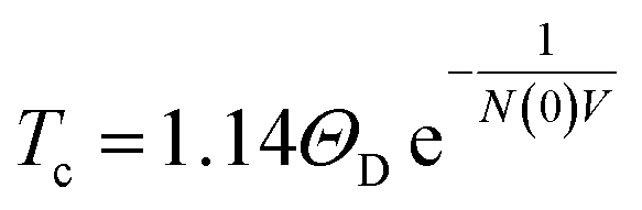 , where Θ_D represents the Debye temperature, N(0) is the electronic density of states near the Fermi level, and V refers to the electron–phonon coupling potential.^4,5 The BCS theory explains the isotope effect perfectly for 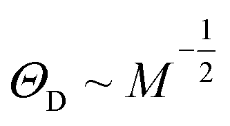, T_c ∼ M^−α, and 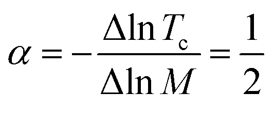.^6,7 Decades later, in 1986, Bednorz and Müller pioneeringly discovered the cuprate Ba–La–Cu–O (BLCO) to be a high-T_c superconductor. To date, the highest T_c record holder of cuprates, obtained by Eggert and Gao et al., is Hg–Ba–Ca–Cu–O with a T_c of 164 K under a high pressure of up to 16 kbar.^8,9 The compounds mentioned above are among many above-liquid-nitrogen-temperature cuprate superconductors classified as Y, Bi, Tl, and Hg series.

Detecting the isotope effect of conventional superconductors only involves the isotope substitution of a few kinds of atoms, which is relatively simple. However, the isotope effect in cuprates is more complex than in conventional superconductors, with the α value changing with the hole-doping concentration.^6,10,11 While the BCS theory based on electron–phonon coupling can explain some of the isotope effects of La series cuprate superconductors, it fails for the isotope effect counterparts in Y, Bi, Tl, and Hg series cuprate superconductors.^6,7,12–14 It is widely accepted that even though electron–phonon coupling could induce high-T_c superconductivity, the cuprates are still believed not to be determined as phonon-mediated.^13–25

Machine learning (ML) has become an essential data-driven research approach that has been rapidly developed in recent years.²⁶ In contrast to traditional methods, ML does not rely on the development of any prior physical knowledge (e.g., Debye temperature or phonon dynamics properties)²⁷ but utilizes data to explore the physical rules, showing outstanding performances in scientific research and industrial design.^28–38 Stanev et al. reported ML models to explore the rule of the superconducting transition temperature.³⁹ Xie et al. applied the sure independence screening and sparsifying operator (SISSO) approach to search for mathematical formulas related to superconductivity with smaller errors.^40,41 In a study by Mori et al., the synthesis of machine-learning-assisted materials was applied to accelerate the exploration of novel thin film superconductors.⁴² These studies have shown the feasibility of utilizing ML for data mining in the search of superconducting materials and inspired us to carry out the present investigation.

Physics-informed neural networks (PINNs)^43,44 are a type of neural network whose training process incorporates physical principles or equations as constraints. This method has various advantages over conventional neural networks, including the capacity to incorporate a system's priorities and the potential to avoid overfitting and enhance generalization. The use of PINNs to handle small data sets, a prevalent issue in many physics-based applications, is one of the primary advantages of this method. By introducing physical restrictions, PINNs may utilize available data to create accurate predictions and enhanced performance. However, the utilization of physical constraints might also result in network limitations. For instance, if the physical equations or rules employed in the network are inaccurate or insufficient, the network's performance may suffer. In addition, the introduction of physical restrictions increases the architecture's complexity, which may necessitate additional processing resources and lengthier training cycles.

Cuprate materials are a significant class of superconducting materials, and the enhancement of their superconducting transition temperature has long been an important area of superconductivity study. Nonetheless, there is currently no developed theoretical model that can correlate the superconducting transition temperature of these materials, which poses significant hurdles for the research community. Consequently, despite the fact that the PINNs approach has yielded outstanding results in a variety of disciplines, it is now inapplicable due to its inability to deal with the superconducting transition temperature of cuprate materials.

Our approach to overcoming this limitation involves designing a feature engineering process based on prior physical knowledge, followed by utilizing manifold learning to determine the direction for material design. We analyzed SHapley Additive exPlanations (SHAP) values and found that shorter covalent bonds and lower hole-doping concentrations are effective ways to enhance the T_c for most materials. To improve the accuracy of our model, we established a cost-sensitive ML model to resolve sample imbalance and an ensemble learning model using two deep neural networks (DNN) with non-correlation characteristics.

We found that tree-based regression models lack the ability to extrapolate the higher superconducting transition temperature outside the dataset's range, while support vector machines (SVMs) rely heavily on challenging feature engineering, and so DNN was finally chosen as our extrapolation model for regression prediction due to the difficulties of feature engineering and the desire to reunite knowledge fragments. We used a Monte Carlo-based test set partitioning strategy to prevent data leakage caused by repetitive optimizations of the test set, hence retaining the generalization performance of the model. However, in our scenario, the inclusion of framework and parameter hyperparameters, as well as Monte Carlo data set partitioning, made optimization particularly difficult; therefore, the Tree-structured Parzen Estimator (TPE) method based on the Bayesian optimization algorithm was employed to perform the optimization.

We then applied the model to predict high-T_c materials and performed virtual high-throughput (VH) screening of superconductors in a larger space. By combining conclusions obtained from domain knowledge, our work resulted in an ML model with specific explanatory capabilities.

2 Methods

2.1 Data source

We chose the Supercon database as our dataset source.⁴⁵ After removing the data without the exact chemical formula, we took the median temperature for those of the same chemical formula corresponding to multiple T_c, as the median was actually obtained in the experiment.⁴⁶ After the screening, 12 340 T_c data were collected, with a small number of materials having structural information from the literature. As shown in Fig. S1,† most of the materials had T_c values of less than 20 K, and only a few materials had critical temperatures greater than 120 K, and the highest T_c material was Hg_0.66Pb_0.34Ba₂Ca_1.98Cu_2.9O_8.4 with T_c = 143 K.

2.2 Feature engineering

Two kinds of descriptors were used in this work, namely the atomic feature set 1 (AFS-1) and atomic feature set 2 (AFS-2). The feature extraction of AFS is based on ‘cell’ processing, in which we define all the elements in the normalization formula as a ‘pseudo cell,’ and its stoichiometric number is the weight of each element. AFS-1 is the symbolic element one-hot encoding based on the properties of the elemental components, it is a vector defined by multidimensional elements as a mapping vector composed of the elements in the chemical formula, and we can view it as a vector with a high dimension. For AFS-1, the dimension of the vector space of the whole feature is equal to the sum of the elements number in the periodic table of elements. In the feature space of AFS-1, the neural network's self-processing of the features might even go beyond the artificially designed descriptors.⁴⁷ AFS-2 was established on the physical properties of the component elements. A file is required and it is used to fill in the characteristics of each element according to the users' domain knowledge. We use this series of physical quantities as descriptors supported by the following superconductivity prior knowledge: (a) according to Zhao et al., T_c may have a relationship with the valence of copper,⁴⁸ and then the Jahn–Teller effect in the superconducting sample;⁴⁹ (b) the mainstream theory of cuprate high-temperature superconductors resonance valence bond theory (RVB),⁵⁰ Zhang–Rice Model (ZRM),⁵¹ and t–J model;⁵² (c) SO(5) supersymmetry theory,⁵³ according to the theory that T_c is most related to the electron-doping concentration; (d) there is a relationship between T_c, the electronic structure (Cu d orbitals or Cu–O chemical bonds), and the magnetic structure (mainly the magnitude of the exchange coupling integral J, and then the correlation energy U).^54–62 In details, (1) superconductivity was obtained by the magnetic exchange interaction and Fermi surface; (2) the impact of Jahn–Teller effect and crystal field restricts the electron number in superconductivity. And (e) the polarons and plasmon, whereby T_c is related to the factor of the conformation of the polarons, hole concentration, and parameters concerning the lattice conformation of a (or the) layered structure.¹⁵ As an excellent descriptor should be universal and accessible, we considered using basic descriptors for mapping basic influencing factors, as shown in Table S1.† AFS-2 was used to calculate the features in the cell. According to the attributes of the input elements, we designed the treatment of the characteristics of doped systems. AFS-1 and AFS-2 were converted into convenient software, with the details given in the ESI.†

3 Results and discussion

3.1 Cost-sensitive classification model

We used the PyCaret library for model selection,⁶³ and then got the first four models to show stable performance for both descriptors, with their 10-fold cross-validation accuracy rates shown in Table 1. Taking the random forest (RF) model for AFS-1 to train as our basic model, the confusion matrix and receiver operating characteristic (ROC) curve are shown in Fig. 1.

Table 1 Accuracy of k-nearest neighbors (KNN) model, decision tree (DT) model, random forest (RF) model, and adaboost (AB) model by using AFS-1, AFS-2, and AFS-1&AFS-2, respectively

Model	AFS-1	AFS-2	AFS-1&AFS-2
KNN	0.9639	0.9548	0.9574
DT	0.9549	0.9434	0.9541
RF	0.9658	0.9599	0.9636
AB	0.9569	0.9541	0.9574

---

Fig. 1 (a) In the confusion matrix, the label ‘0’ represents the high-T_c materials, and the label ‘1’ represents the low-T_c materials. (b) According to the receiver operating characteristic (ROC) of classification, the larger the area under the ROC curve (AUC), the better the model's performance is.

The critical temperature of liquid nitrogen, 77 K, was adopted as the temperature boundary, i.e., low T_c is below 77 K while high T_c is above it. In Fig. 1, we got the confusion matrix on a random test and the AUC score of about 0.98, but there were two notable issues in the analysis of the classified datasets: (a) the uneven distribution of samples, i.e., 1233 high-T_c materials versus 11 107 low-T_c in the dataset; (b) the two materials in the misjudgment cost model were different, that is, the model predicted high-T_c for low-T_c materials penalty (serious error) versus the low-T_c predicted for high-T_c materials penalty (general error), so we applied an ML model adjustment by setting an additional penalty of 1.5 times to serious errors more than the general error, and thus obtained the ideal threshold by observing the cost function curve. As shown in Fig. 2, the lowest point of the cost curve was selected as the threshold of the RF model classifier. Since even a trained model has a certain degree of randomness, we should find the interval with the best threshold near the lowest value. After passing the sliding threshold test, the threshold range was determined to be 0.44 ± 0.03, and within this threshold interval, the serious error was reduced to 29 and the general error rose to 55, while the accuracy was not compromised. See the ESI† for the graph of the sliding threshold interval.

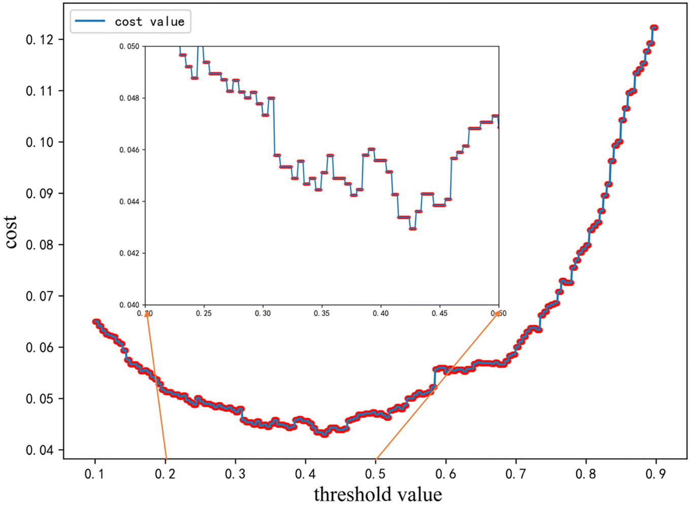Fig. 2 Misclassification inequality cost function curve, where the local optimal threshold value was around 0.42 and sliding thresholds were needed to search the global optimal threshold value.

3.2 Situation-adaptive regression model

From the regression analysis (Fig. 3 and S5†), we can find that the DNN trained based on AFS-1 had less error than AFS-2, but that does not necessarily mean that AFS-1 was better (see ESI†). For example, for Pr, Tb, Ho, Tm, and Sm elements, the DNN based on AFS-2 predicted their T_c to be 0 K, but the DNN based on AFS-1 gave T_c values of 15.91, 9.22, 8.88, 17.24, and 6.34 K, though these materials were not superconducting.⁶⁴

Fig. 3 (a) DNN trained by using AFS-1 results: R² = 0.95, RMSE = 6.08 K, MAE = 3.08 K. (b) DNN trained by using AFS-2 results: R² = 0.93, RMSE = 7.35 K, MAE = 3.73 K.

3.3 Model interpretation

RF model can extract the importance of features according to the branching situation of sub-trees during training, and here we calculated the SHAP value in order to refine the influence of the feature on the target value and analyzed the SHAP value of the top 20 importance features from AFS-2.⁶⁵

In Fig. 4, the top-to-bottom features represent the degree of influence on T_c. We found the feature having the greatest impact on T_c was the longest value of the covalent bond in a cell. When the distribution value of this feature was lowered, the T_c increased, as this feature was mentioned four times in five prior knowledge. From the RVB theory, we can qualitatively state that the J/t value in the t–J model will decrease when the ionic bond is short. The second important feature was the average number of unfilled electrons in a cell, whose high values (in red) appeared near the minimum and small SHAP values. For hole doping in cuprates, the influence of the concentration is such that T_c increases when the hole concentration decreases, but with an optimal concentration range, and overdoping will reduce the T_c value. This is qualitatively consistent with the inference of SO(5) theory when the holes concentration was high, and experiments show that the properties of high-temperature superconductors are metalized rather than insulators, so electrons are easy to hop and the J/t value will also be affected. This is consistent with the analysis in the first feature, so the first two features selected by the ML were self-consistent in theory. The third important feature was the maximum row value of an element in the periodic table, reflecting the influence of the cycle of the elements on T_c. As a rule summarized by ML, the upper rows of the periodic table have a greater influence on T_c.

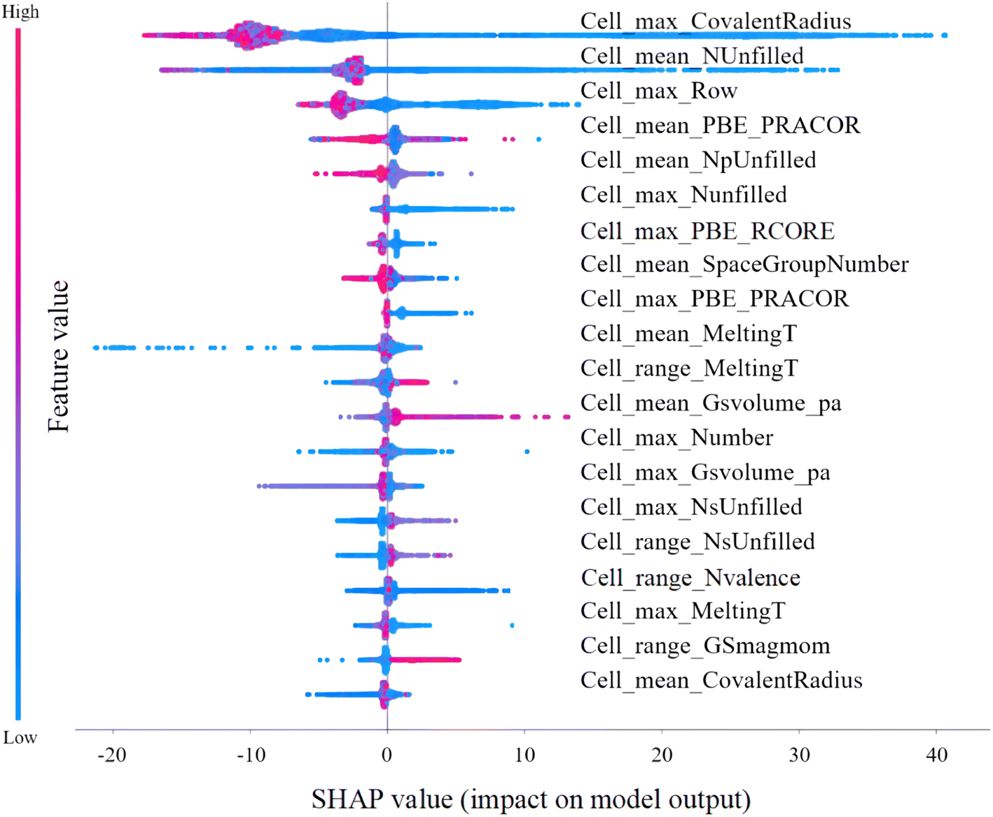Fig. 4 SHAP values of top 20 important features of AFS-2, which indicate the impact of the feature values on the variation on T_c.

Manifold learning is considered to be an important way to understand high-dimensional data structures. Since the t-distributed stochastic neighbor embedding (T-SNE) reduction visualization data overlap the least, this was selected as the dimensionality reduction method (Fig. S7†). In Fig. 5, it can be found that there was a great correlation between the content of Cu reflected in this two-dimensional mapping space and the T_c, so this was indeed a suitable choice to set Cu-based (cuprate) superconducting materials by DNN. The Fe content was reflected in the middle of the manifold region, which indicated that the T_c of Fe-based superconductors is not as high as that of Cu-based superconductors, and this was indeed the case in the experiments.^67–69 In terms of the stoichiometry weight of the elements, there are some elements that are restricted to specific intervals. For example, the O content in cuprates should be within a proper range. Otherwise, it will transform into semiconductors or even insulators,^70–73 and a similar phenomenon also exists for Cu and Fe. In contrast, Ba and La were obviously different, as they were scattered in various parts of the manifold space without specific intervals. The characteristic dying in the manifold and the distribution of target values can provide component references in the material design.

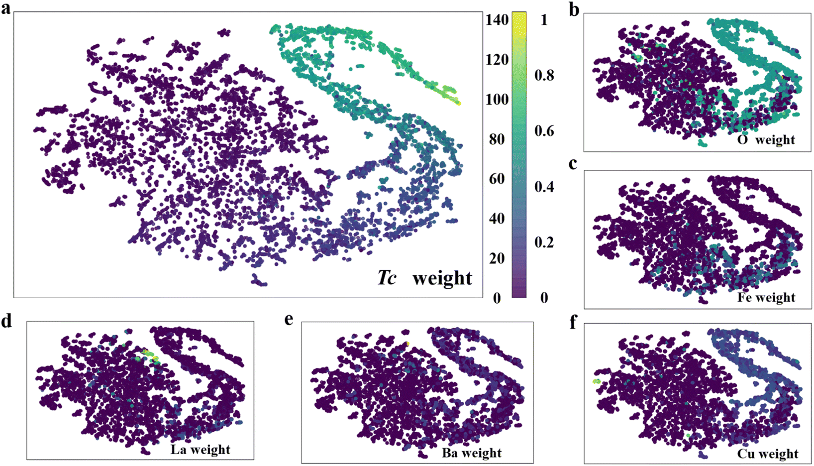Fig. 5 Two-dimensional mapping space under the dimension reduction of t-distributed stochastic neighbor embedding (T-SNE).⁶⁶ (a) T_c by the materials weight mapping in this two-dimensional space. (b)–f. O, Fe, La, Ba, and Cu stoichiometric numbers by the materials' weight mapping in this two-dimensional space. The color column represents the T_c (left) and component (right) in materials.

3.4 Model application

The predicted values of the average from two neural networks were chosen as the prediction basis for an ensemble ML model, and we named it e-DNN. Materials in the Materials Project (MP) database were predicted by applying the e-DNN model,⁷⁴ with the distribution of T_c, and the best candidates are shown in Fig. S2.† It can be seen that the distribution of T_c was the same as the distribution of the training data. The complete prediction document is given in the ESI.†

In the set of predictions for the MP database, we found evidence of some possible high-T_c materials from their electronic structure. For known cuprate superconductors, flat-bands below the energy of the highest occupied electronic state lead to a large peak in the electronic to help enhance T_c; more importantly, DOS peaks close to E_F due to the Van Hove singularity may also enhance T_c.⁷⁵ As shown in Fig. 6, most of our predicted cuprate candidate samples have peaks near the E_F of DOS, which greatly complies with the laws of physics, as we discussed in 2.2.

Fig. 6 Examples of some candidate cuprates with T_c about 77 K in the MP database and their electronic density of states (DOS) from MP. (a) Li₄Cu₃SbO₈ (89.23 K); (b) Li₄NbCu₃O₈ (98.62 K); (c) CaCuAsO₅ (61.78 K); (d) Ba₂DyCu₃O₇ (89.99 K); (e) Li₄Cu₃TeO₈ (87.98 K); (f) CaCuAs₂O₇ (79.73 K).

There are some data with missing T_c labels in the Supercon database, though these existing materials are feasible for experimental synthesis (Table 2). The average absolute value difference of two DNN predicted results was about 10 K, as there was a huge disparity in the prediction results of some data. These data can be roughly divided into three categories: experiments under high pressure, non-superconducting materials, and material information flaws (some data might have been incorrectly inputted into the database).

Table 2 Predicted value of some unlabeled data in our training data. The complete prediction document is given in the ESI

Formula	Tc (AFS-1)	Tc (AFS-2)
La1.8Nd0.2Ba2Ca0.4Cu4.4O7.183	103.18	97.53
Bi1.6Pb0.3V0.1Sr2Ca2Cu3O9.92	96.31	88.24
Bi1.6Pb0.35V0.05Sr2Ca2Cu3O9.92	94.68	89.26
Tb1Ba2Cu3O7	92.83	88.12
Bi2Sr2Ca0.5Er0.5Cu2O8	90.35	83.66
Y1Ba2Cu3H0.43O6.91	89.46	80.12
Y0.76Lu0.24Ba2Cu4O8	87.91	89.94
Ba1.6Sr0.4Yb1Cu3O6.42	87.72	80.25
Ba1.6Sr0.4Yb1Cu3O6.26	86.72	81.17
Y0.8Eu0.2Ba2Cu3O7	85.99	81.57
Eu1Ba1Sr0.6Ca0.4Cu3O6.95	85.30	95.47
Ba1.6Sr0.4Yb1Cu3O6.15	85.29	82.43
Y1Ba2Cu3O6.975	84.38	80.67
Er1Ba2Cu3O6.95	84.18	88.58
Er1Ba2Cu3O6.88	84.01	90.65
Cu9.5Sr2Ca8Cr0.5O21.05	83.51	80.24
Ba1.6Sr0.4Yb0.85Ca0.15Cu3O6.17	82.75	80.92
Pb0.5Sr2Ca1Cu2.5O7.4	82.12	83.19
Ca0.1Ba1.65Nd1.25Cu3O7.03	81.70	86.93
Ba1.6Sr0.4Yb1Cu3O5.97	81.09	88.07
Pb2Sr2Y0.5Ca0.5Cu3O9.4	80.15	85.54

---

In statistics, a confidence interval (CI) is a range of estimates for an unknown parameter, computed at a designated confidence level. The CI shows the degree of confidence in the measured value of the parameter, e.g., a 95% confidence level is most common, but other levels (such as 90% or 99%) are sometimes used.

The CI is calculated by the following formula:

{upper, lowerbound} = X ± z × RMSE.

where X is the predicted value in this case, and z is the standard score corresponding to the 95% confidence interval obtained from the standard normal distribution. For example, the CI of Y₁Ba₂Cu₃O_6.975 was {72.46, 96.30} by AFS-1, and {66.26, 95.08} by AFS-2. The experimental value of Y₁Ba₂Cu₃O₇ was 93 K,⁷⁶ which was in the ranges of both the CIs.

Based on the distribution characteristics of the datasets, a series of virtual samples could be designed for prediction.^77,78 Here, we took the samples containing the Hg–Pb–Ba–Ca–Cu–O composition as an example to perform a VH search. As a result of Fig. 7, Hg_0.13Pb_0.09Ba_0.32Ca_0.422Cu_0.4O₁ was found to have the highest T_c of 152 K, which represents a prediction of the optimal value generated by the combination of five metal elements and the O element in the chemical formula. There also are many other frequently appearing elements in the data set, such as Sr and Y; therefore, VH samples can also be set up by the above methods, but we suggest that the Cu–O base should be used and combined with other elements to construct virtual samples, and then to predict the composition of the compounds of interest (the element richness information and VH design method are given in the ESI†).

Fig. 7 Predicted values for partial VH samples. (a) Virtual sample prediction results with Cu as independent variables, and where blue and orange curves represent the highest and lowest predicted values, respectively. (b) For the VH prediction when the Cu element content was 0.4, most of the data were still below 120 K, and only 170 samples had T_c predictions above 140 K, and there were only five samples with predicted results exceeding 150 K.

4 Conclusion

In summary, we developed cost-sensitive classification and situation-adaptive regression ML models to mitigate prediction risks. Two descriptors, AFS-1 and AFS-2, were chosen for comparison and supplementation in predicting T_c for known components as well as for unknown T_c and VH screening. SHAP analysis revealed that shortening covalent bond lengths and increasing hole-doping concentrations are the two physical factors that can increase the T_c. Our work provides a practical and accurate ML model for predicting the T_c of unknown materials, and can offer valuable guidance for future experiments.

Code availability

The code and datasets for our work are available online from the following GitHub link. https://github.com/Suth-ICQMS/AFS.

Conflicts of interest

There are no conflicts to declare.

Acknowledgements

This work was supported by the National Natural Science Foundation of China (52271007, 12074241, 52130204, 11929401), the Science and Technology Commission of Shanghai Municipality (22XD1400900, 21JC1402600, 21JC1402700, 20501130600), High Performance Computing Center, Shanghai Technical Service Center of Science and Engineering Computing, Shanghai University, Shanghai Supercomputer Center, and Key Research Project of Zhejiang Laboratory (No. 2021PE0AC02), the Key Research and Development Program of Shaanxi Province (Grant No. 2021GXLH-Z-065). We also would like to acknowledge Dr Ouyang Runhai for discussions.

References

1. H. K. Onnes, in Proceedings koninklijke akademie van wetenschappen te amsterdam, 1911, vol. 13, pp. 1274–1276.
2. C. A. Reynolds, B. Serin, W. H. Wright and L. B. Nesbitt, Superconductivity of Isotopes of Mercury, Phys. Rev., 1950, 78, 487.
3. E. Maxwell, Isotope Effect in the Superconductivity of Mercury, Phys. Rev., 1950, 78, 477.
4. J. Bardeen, L. N. Cooper and J. R. Schrieffer, Microscopic Theory of Superconductivity, Phys. Rev., 1957, 106, 162–164.
5. J. Bardeen, L. N. Cooper and J. R. Schrieffer, Theory of Superconductivity, Phys. Rev., 1957, 108, 1175–1204.
6. Z.-Z. Li, Solids Theory: A Postgraduate Teaching Book, High Education Press, 2002, vol. 2.
7. J. R. Schrieffer, Theory Of Superconductivity, CRC Press, Boca Raton, 2019.
8. J. H. Eggert, J. Z. Hu, H. K. Mao, L. Beauvais, R. L. Meng and C. W. Chu, Compressibility of the HgBa₂Ca_n−1Cu_nO_2n+2+δ(n = 1, 2, 3) high-temperature superconductors, Phys. Rev. B: Condens. Matter Mater. Phys., 1994, 49, 15299–15304.
9. L. Gao, Y. Y. Xue, F. Chen, Q. Xiong, R. L. Meng, D. Ramirez, C. W. Chu, J. H. Eggert and H. K. Mao, Superconductivity up to 164 K in HgBa₂Ca_m−1Cu_mO_2m+2+δ (m =1, 2, 3) under quasihydrostatic pressures, Phys. Rev. B: Condens. Matter Mater. Phys., 1994, 50, 4260–4263.
10. D. M. Ginsberg, Physical Properties Of High Temperature Superconductors, World Scientific, 1998, vol. 1.
11. U. Rössler, Solid State Theory: An Introduction, Springer Science & Business Media, 2013.
12. O. Isayev, D. Fourches, E. N. Muratov, C. Oses, K. Rasch, A. Tropsha and S. Curtarolo, Materials Cartography: Representing and Mining Materials Space Using Structural and Electronic Fingerprints, Chem. Mater., 2015, 27, 735–743.
13. A. Lanzara, P. V. Bogdanov, X. J. Zhou, S. A. Kellar, D. L. Feng, E. D. Lu, T. Yoshida, H. Eisaki, A. Fujimori, K. Kishio, J.-I. Shimoyama, T. Noda, S. Uchida, Z. Hussain and Z.-X. Shen, Evidence for ubiquitous strong electron–phonon coupling in high-temperature superconductors, Nature, 2001, 412, 510–514.
14. R. K. Pandey, S. P. Singh and P. Singh, A Possible Explanation of Critical Temperature and Isotope Effect Coefficient of High T_c Cuprate Superconductors, J. Supercond., 1998, 11, 663–665.
15. V. Z. Kresin and S. A. Wolf, Colloquium : Electron-lattice interaction and its impact on high T_c superconductivity, Rev. Mod. Phys., 2009, 81, 481–501.
16. D. Oh, D. Song, Y. Kim, S. Miyasaka, S. Tajima, J. M. Bok, Y. Bang, S. R. Park and C. Kim, B_1g-Phonon Anomaly Driven by Fermi Surface Instability at Intermediate Temperature in YBa₂Cu₃O_7−δ, Phys. Rev. Lett., 2021, 127, 277001.
17. A. Ramos-Alvarez, N. Fleischmann, L. Vidas, A. Fernandez-Rodriguez, A. Palau and S. Wall, Probing the lattice anharmonicity of superconducting YBa₂Cu₃O₇ via phonon harmonics, Phys. Rev. B, 2019, 100, 184302.
18. S. Sarkar, M. Grandadam and C. Pépin, Anomalous softening of phonon dispersion in cuprate superconductors, Phys. Rev. Res., 2021, 3, 013162.
19. D. M. Newns and C. C. Tsuei, Fluctuating Cu–O–Cu bond model of high-temperature superconductivity, Nat. Phys., 2007, 3, 184–191.
20. W. Hu, S. Kaiser, D. Nicoletti, C. R. Hunt, I. Gierz, M. C. Hoffmann, M. Le Tacon, T. Loew, B. Keimer and A. Cavalleri, Optically enhanced coherent transport in YBa₂Cu₃O_6.5 by ultrafast redistribution of interlayer coupling, Nat. Mater., 2014, 13, 705–711.
21. R. Mankowsky, A. Subedi, M. Först, S. O. Mariager, M. Chollet, H. T. Lemke, J. S. Robinson, J. M. Glownia, M. P. Minitti, A. Frano, M. Fechner, N. A. Spaldin, T. Loew, B. Keimer, A. Georges and A. Cavalleri, Nonlinear lattice dynamics as a basis for enhanced superconductivity in YBa₂Cu₃O_6.5, Nature, 2014, 516, 71–73.
22. G.-H. Gweon, T. Sasagawa, S. Y. Zhou, J. Graf, H. Takagi, D.-H. Lee and A. Lanzara, An unusual isotope effect in a high-transition-temperature superconductor, Nature, 2004, 430, 187–190.
23. Q. Xiong, J. W. Chu, Y. Y. Sun, H. H. Feng, S. Bud'ko, P. H. Hor and C. W. Chu, High-pressure study of the anomalous isotope effect in La_2−xA_xCuO₄ with A = Sr or Ba, Phys. Rev. B: Condens. Matter Mater. Phys., 1992, 46, 581–584.
24. P. Boolchand, R. N. Enzweiler, I. Zitkovsky, J. Wells, W. Bresser, D. McDaniel, R. L. Meng, P. H. Hor, C. W. Chu and C. Y. Huang, Softening of Cu–O vibrational modes as a precursor to onset of superconductivity in EuBa₂Cu₃O_7−δ, Phys. Rev. B: Condens. Matter Mater. Phys., 1988, 37, 3766–3769.
25. B. K. Chakraverty, Possibility of insulator to superconductor phase transition, J. Phys. Lett., 1979, 40, 99–100.
26. T.-Y. Zhang, New tool in the box, J. Mater. Inf., 2021, 1, 1.
27. R. Iten, T. Metger, H. Wilming, L. del Rio and R. Renner, Discovering Physical Concepts with Neural Networks, Phys. Rev. Lett., 2020, 124, 010508.
28. G. Csányi, T. Albaret, M. C. Payne and A. De Vita, Learn on the Fly”: A Hybrid Classical and Quantum-Mechanical Molecular Dynamics Simulation, Phys. Rev. Lett., 2004, 93, 175503.
29. R. Jinnouchi, F. Karsai and G. Kresse, On-the-fly machine learning force field generation: Application to melting points, Phys. Rev. B, 2019, 100, 014105.
30. R. Jinnouchi, J. Lahnsteiner, F. Karsai, G. Kresse and M. Bokdam, Phase Transitions of Hybrid Perovskites Simulated by Machine-Learning Force Fields Trained on the Fly with Bayesian Inference, Phys. Rev. Lett., 2019, 122, 225701.
31. Y. Zhang, Q. Tang, Y. Zhang, J. Wang, U. Stimming and A. A. Lee, Identifying degradation patterns of lithium ion batteries from impedance spectroscopy using machine learning, Nat. Commun., 2020, 11, 1706.
32. T. Yokoi, Y. Noda, A. Nakamura and K. Matsunaga, Neural-network interatomic potential for grain boundary structures and their energetics in silicon, Phys. Rev. Mater., 2020, 4, 014605.
33. Y. Zhuo, A. Mansouri Tehrani, A. O. Oliynyk, A. C. Duke and J. Brgoch, Identifying an efficient, thermally robust inorganic phosphor host via machine learning, Nat. Commun., 2018, 9, 4377.
34. Y. Long, J. Ren and H. Chen, Unsupervised Manifold Clustering of Topological Phononics, Phys. Rev. Lett., 2020, 124, 185501.
35. P. Baldi, P. Sadowski and D. Whiteson, Searching for exotic particles in high-energy physics with deep learning, Nat. Commun., 2014, 5, 4308.
36. A. Andreassen, I. Feige, C. Frye and M. D. Schwartz, JUNIPR: a framework for unsupervised machine learning in particle physics, Eur. Phys. J. C, 2019, 79, 102.
37. L. Li, J. C. Snyder, I. M. Pelaschier, J. Huang, U.-N. Niranjan, P. Duncan, M. Rupp, K.-R. Müller and K. Burke, Understanding machine-learned density functionals, Int. J. Quantum Chem., 2016, 116, 819–833.
38. T. Su, Y. Cui, Z. Lian, M. Hu, M. Li, W. Lu and W. Ren, Physics-Based Feature Makes Machine Learning Cognizing Crystal Properties Simple, J. Phys. Chem. Lett., 2021, 12, 8521–8527.
39. V. Stanev, C. Oses, A. G. Kusne, E. Rodriguez, J. Paglione, S. Curtarolo and I. Takeuchi, Machine learning modeling of superconducting critical temperature, npj Comput. Mater., 2018, 4, 1–14.
40. R. Ouyang, S. Curtarolo, E. Ahmetcik, M. Scheffler and L. M. Ghiringhelli, SISSO: A compressed-sensing method for identifying the best low-dimensional descriptor in an immensity of offered candidates, Phys. Rev. Mater., 2018, 2, 083802.
41. S. R. Xie, G. R. Stewart, J. J. Hamlin, P. J. Hirschfeld and R. G. Hennig, Functional form of the superconducting critical temperature from machine learning, Phys. Rev. B, 2019, 100, 174513.
42. I. Ohkubo, Z. Hou, J. N. Lee, T. Aizawa, M. Lippmaa, T. Chikyow, K. Tsuda and T. Mori, Realization of closed-loop optimization of epitaxial titanium nitride thin-film growth via machine learning, Mater. Today Phys., 2021, 16, 100296.
43. E. Samaniego, C. Anitescu, S. Goswami, V. M. Nguyen-Thanh, H. Guo, K. Hamdia, X. Zhuang and T. Rabczuk, An energy approach to the solution of partial differential equations in computational mechanics via machine learning: concepts, implementation and applications, Comput. Methods Appl. Mech. Eng., 2020, 362, 112790.
44. L. Yang, X. Meng and G. E. Karniadakis, B-PINNs: Bayesian physics-informed neural networks for forward and inverse PDE problems with noisy data, J. Comput. Phys., 2021, 425, 109913.
45. NIMS Materials Database(MatNavi) – SuperCon, National Institute for Materials Science.
46. J. Nelson and S. Sanvito, Predicting the Curie temperature of ferromagnets using machine learning, Phys. Rev. Mater., 2019, 3, 104405.
47. D. Jha, L. Ward, A. Paul, W. Liao, A. Choudhary, C. Wolverton and A. Agrawal, ElemNet: Deep Learning the Chemistry of Materials From Only Elemental Composition, Sci. Rep., 2018, 8, 17593.
48. Z. Zhao, L. Chen, C. Cui, Y. Huang, J. Liu, G. Chen, S. Li, S. Guo and Y. He, High critical temperature superconductivity of Sr(Ba)–La–Cu oxides, Sci. Bull., 1987, 177–179.
49. H. Keller, A. Bussmann-Holder and K. A. Müller, Jahn–Teller physics and high-T_c superconductivity, Mater. Today, 2008, 11, 38–46.
50. P. W. Anderson, The Resonating Valence Bond State in La₂CuO₄and Superconductivity, Science, 1987, 235, 1196–1198.
51. F. C. Zhang and T. M. Rice, Effective Hamiltonian for the superconducting Cu oxides, Phys. Rev. B: Condens. Matter Mater. Phys., 1988, 37, 3759–3761.
52. M. Ogata and H. Fukuyama, The t–J model for the oxide high-T_c superconductors, Rep. Prog. Phys., 2008, 71, 036501.
53. S.-C. Zhang, A Unified Theory Based on SO(5) Symmetry of Superconductivity and Antiferromagnetism, Science, 1997, 275, 1089–1096.
54. J. Hu and J. Yuan, Robustness of s-wave pairing symmetry in iron-based superconductors and its implications for fundamentals of magnetically driven high-temperature superconductivity, Front. Phys., 2016, 11, 117404.
55. J. C. S. Davis and D.-H. Lee, Proc. Natl. Acad. Sci. U. S. A., 2013, 110, 17623–17630.
56. C. Le, S. Qin and J. Hu, Electronic physics and possible superconductivity in layered orthorhombic cobalt oxychalcogenides, Sci. Bull., 2017, 62, 563–571.
57. D. C. Johnston, The puzzle of high temperature superconductivity in layered iron pnictides and chalcogenides, Adv. Phys., 2010, 59, 803–1061.
58. J. Hu and C. Le, A possible new family of unconventional high temperature superconductors, Sci. Bull., 2017, 62, 212–217.
59. J. Hu, Identifying the genes of unconventional high temperature superconductors, Sci. Bull., 2016, 61, 561–569.
60. J. Hu, C. Le and X. Wu, Predicting Unconventional High-Temperature Superconductors in Trigonal Bipyramidal Coordinations, Phys. Rev. X, 2015, 5, 041012.
61. S. G. Ovchinnikov and E. I. Shneyder, The Interplay of Phonon and Magnetic Mechanism of Pairing in Strongly Correlated Electron System of High-TcCuprates, J. Supercond. Novel Magn., 2010, 23, 733–736.
62. J. Hu and H. Ding, Local antiferromagnetic exchange and collaborative Fermi surface as key ingredients of high temperature superconductors, Sci. Rep., 2012, 2, 381.
63. M. Ali, PyCaret: An open source, low-code machine learning library in Python, PyCaret Version.
64. Type 1 Superconductors, http://www.superconductors.org/Type1.htm.
65. S. M. Lundberg and S.-I. Lee, in Advances in Neural Information Processing Systems, Curran Associates, Inc., 2017, vol. 30.
66. L. van der Maaten and G. Hinton, Viualizing data using t-SNE, J. Mach. Learn. Res., 2008, 9, 2579–2605.
67. X. Zhao, F. Ma, Z.-Y. Lu and T. Xiang, A FeSe₂(A = Tl, K, Rb, or Cs): Iron-based superconducting analog of the cuprates, Phys. Rev. B, 2020, 101, 184504.
68. X. Chen, P. Dai, D. Feng, T. Xiang and F.-C. Zhang, Iron-based high transition temperature superconductors, Natl. Sci. Rev., 2014, 1, 371–395.
69. C. Wang, L. Li, S. Chi, Z. Zhu, Z. Ren, Y. Li, Y. Wang, X. Lin, Y. Luo, S. Jiang, X. Xu, G. Cao and Z. Xu, Thorium-doping–induced superconductivity up to 56 K in Gd_1−xTh_xFeAsO, EPL, 2008, 83, 67006.
70. R. J. Cava, B. Batlogg, C. H. Chen, E. A. Rietman, S. M. Zahurak and D. Werder, Oxygen stoichiometry, superconductivity and normal-state properties of YBa₂Cu₃O_7−δ, Nature, 1987, 329, 423–425.
71. J. D. Jorgensen, B. W. Veal, W. K. Kwok, G. W. Crabtree, A. Umezawa, L. J. Nowicki and A. P. Paulikas, Structural and superconducting properties of orthorhombic and tetragonal YBa₂Cu₃O_7−x : The effect of oxygen stoichiometry and ordering on superconductivity, Phys. Rev. B: Condens. Matter Mater. Phys., 1987, 36, 5731–5734.
72. R. J. Cava, A. W. Hewat, E. A. Hewat, B. Batlogg, M. Marezio, K. M. Rabe, J. J. Krajewski, W. F. Peck and L. W. Rupp, Structural anomalies, oxygen ordering and superconductivity in oxygen deficient Ba₂YCu₃O_x, Phys. C, 1990, 165, 419–433.
73. J. D. Jorgensen, B. W. Veal, A. P. Paulikas, L. J. Nowicki, G. W. Crabtree, H. Claus and W. K. Kwok, Structural properties of oxygen-deficient YBa₂Cu₃O_7−δ, Phys. Rev. B: Condens. Matter Mater. Phys., 1990, 41, 1863–1877.
74. A. Jain, S. P. Ong, G. Hautier, W. Chen, W. D. Richards, S. Dacek, S. Cholia, D. Gunter, D. Skinner, G. Ceder and K. A. Persson, Commentary: The Materials Project: A materials genome approach to accelerating materials innovation, APL Mater., 2013, 1, 011002.
75. J. E. Hirsch and D. J. Scalapino, Enhanced Superconductivity in Quasi Two-Dimensional Systems, Phys. Rev. Lett., 1986, 56, 2732–2735.
76. M. K. Wu, J. R. Ashburn, C. J. Torng, P. H. Hor, R. L. Meng, L. Gao, Z. J. Huang, Y. Q. Wang and C. W. Chu, Superconductivity at 93 K in a new mixed-phase Y–Ba–Cu–O compound system at ambient pressure, Phys. Rev. Lett., 1987, 58, 908–910.
77. W. P. Walters, M. T. Stahl and M. A. Murcko, Virtual screening—an overview, Drug Discovery Today, 1998, 3, 160–178.
78. C. Wen, Y. Zhang, C. Wang, D. Xue, Y. Bai, S. Antonov, L. Dai, T. Lookman and Y. Su, Machine learning assisted design of high entropy alloys with desired property, Acta Mater., 2019, 170, 109–117.

---

Footnotes

† Electronic supplementary information (ESI) available. See DOI: https://doi.org/10.1039/d3ra02848h

‡ Both authors contribute equally to this work.

---