Reinforcement learning in crystal structure prediction

Abstract

Crystal Structure Prediction (CSP) is a fundamental computational problem in materials science. Basin-hopping is a prominent CSP method that combines global Monte Carlo sampling to search over candidate trial structures with local energy minimisation of these candidates. The sampling uses a stochastic policy to randomly choose which action (such as a swap of atoms) will be used to transform the current structure into the next. Typically hand-tuned for a specific system before the run starts, such a policy is simply a fixed discrete probability distribution of possible actions, which does not depend on the current structure and does not adapt during a CSP run. We show that reinforcement learning (RL) can generate a dynamic policy that both depends on the current structure and improves on the fly during the CSP run. We demonstrate the efficacy of our approach on two CSP codes, FUSE and MC-EMMA. Specifically, we show that, when applied to the autonomous exploration of a phase field to identify the accessible crystal structures, RL can save up to 46% of the computation time.

---

1 Introduction

The properties of materials are controlled by their composition and structure. Crystal structure prediction (CSP)^1–3 has thus been the focus of attention because it enables selection of new materials for synthesis by estimating the energetic stability of the resulting structure. The predicted structure also allows property prediction, creating a potential screening workflow. Given the combinatorial challenge posed by the scale of the number of potential compositions, unit cell dimensions, and spatial atomic locations, a range of successful approaches based on heuristic exploration of the potential energy surface (PES) have been developed to date.^4–8 These approaches use algorithms that rapidly generate many trial crystal structures and assess their energies by subsequent local minimisation to identify those structures lying in energy minima on the PES, targeting identification of the global minimum. Every CSP code has its own algorithm and parameterisation, which is characterised by the implemented decision-making process (referred to here as the policy) used to generate trial structures. Our hypothesis is that there is no universal policy for all materials compositions, because of the diversity of possible structures and chemistries. We explore the dynamic generation of an efficient policy on the fly by reinforcement learning (RL) – a machine learning paradigm that formalises learning by trial and error – during the CSP run. RL has been applied to a number of chemical problems^9,10 such as protein folding,¹¹ molecular geometry optimisation,¹² and chemical reaction planning and optimisation.^13,14

We focus on basin-hopping (BH),¹⁵ which is a popular choice for CSP.^16–18 In the BH approach, Monte Carlo (MC) sampling is used to generate possible crystal structures at a given composition. For each generated structure, a local energy minimisation is performed to find the nearest minimum. Given the locally optimised crystal structure with its calculated energy, the code will have a set of possible actions that generate the next trial structure according to a set of deterministic or probabilistic rules. Intuitively, the choice of action will determine how “far” the new trial structure is from the current structure on the PES of that composition. For example, a “local action” may swap two atoms, and a more transformative action may replace the current structure with a new randomly created one (i.e., this action “starts the search again”). A typical policy would be a fixed discrete probability distribution of actions, which is used to randomly draw an action every time BH generates a trial structure. While such policies can effectively balance actions with a good tuning of action probabilities, which requires historic data and is not trivial, they also remain fixed during the run and are applied independently of the current structure or other contextual factors.

Compared to the typical case of a fixed policy that does not depend on the current structure, the RL approach that we develop and evaluate in this paper makes two changes. Firstly, our policies depend on the current structure, in particular the policy uses the calculated energy to help decide which action to take. Secondly, our policies are improved on the fly during a CSP run, thus removing the need for costly and composition-specific hand tuning.

RL algorithms adhere to the principles of Markov Decision Processes¹⁹ and operate on states, actions, and rewards. In a given state, a decision is chosen for this state and then the corresponding action is taken. By taking this action, a reward is obtained (positive, negative, or zero), and the state is updated according to the underlying dynamics of the RL problem. The goal of RL is to obtain policies, i.e., (possibly stochastic) mappings from states to actions, which maximise the expected long-term aggregated reward. The state space that we use to allow the policy to condition on the current structure is defined by the calculated energy of the structure. The calculated energy is clearly a very important “feature” of the structure, and other features could also be incorporated into the state space. The available actions that we consider are based on the existing CSP codes that we apply our approach to. The reward in the simplest case is the reduction of the calculated energy between the current and the trial structure. In addition to rewarding those actions that produce structures with lower energies, we also introduce penalties to disincentivise certain outcomes such as repeating structures.

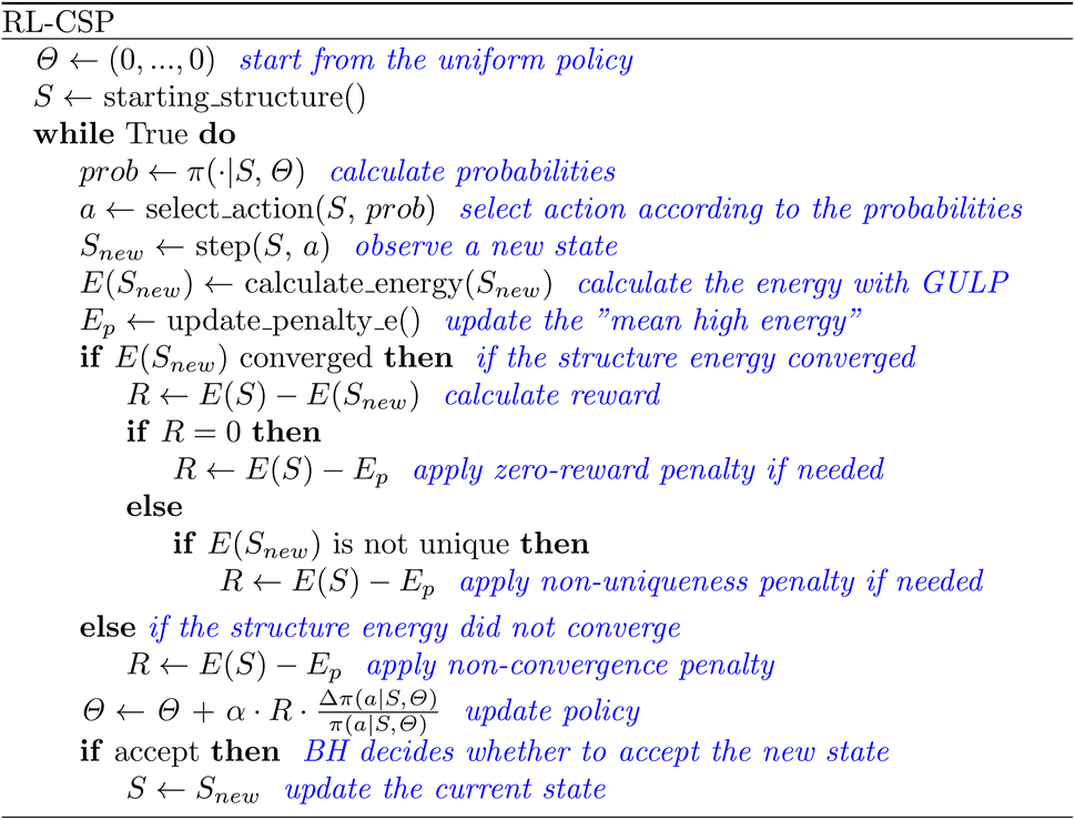
We apply RL to basin-hopping CSP by adapting and implementing the reinforcement learning algorithm REINFORCE,^20,21 which is based on “policy gradients”. With this approach, the policy is parameterized, and the parameters of the policy are improved over time using gradient-based approaches, where the gradients are based on recent experience of the current policy so that actions that led to desirable outcomes are likely to be used again in similar situations. Intuitively, the RL algorithm leverages its past experience to select good actions when similar situations are encountered again as the run proceeds. We refer to this variation of REINFORCE in the CSP context as RL-CSP and illustrate it in Fig. 1.

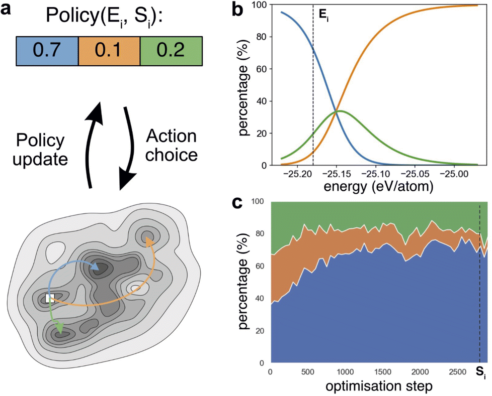Fig. 1 Action selection in RL-CSP. (a) Illustrates the RL-SCP approach for a simplified schematic case where one of three possible actions denoted by orange, green, and blue can be taken to generate a new structure. The actions are chosen at random from a probability distribution of actions that constitutes a policy. This policy dynamically evolves from one optimisation step S_i to another and depends on the energy level E_i of the current structure. The policy is updated after each step according to the reward associated with the outcome of the selected action. The reward function formally captures the desirability of the action choice made and is used by RL-CSP to update the policy. In this illustration, the green and blue actions lead to lower energy structures compared to E_i, which then generate positive rewards. The orange action leads to a structure with an energy higher than E_i and receives a negative reward. This approach leads to an adaptable and dynamic decision making, where action selection depends on structure through its energy (b) and is updated on the fly (c). (a) shows the policy that defines the probability distribution of actions at step S_i when the current structure has the energy E_i. The greyscale potential energy landscape shows the current structure S_i as a square and three coloured arrows leading to three local minima that will be attained after applying one of the three actions. (b) displays how the probability distribution of actions at step S_i depends on the energy with E_i identified by the dashed line. (c) shows how the probability distribution of actions for the structure with energy E_i evolves with time and the dashed line identifies step S_i.

2 Methods

2.1 RL-CSP

In RL-CSP the set of actions is discrete and consists of the limited number of n actions a₁,…, a_n. These actions are the set of moves specific to the CSP code that the algorithm uses to go from one structure to another.

2.1.1 State space. For our choice of state space, we use the current structure as the state and its energy as a feature, since it is intuitively an important factor in deciding which actions are likely to be good for the current structure and is computed as part of the BH routines and therefore does not add an unnecessary overhead. Energy is normalised via Z-score normalization²² to ensure that RL-CSP will work with the same set of hyperparameters across a range of compositions, as the range of possible energies changes between compositions.

2.1.2 Reward. In our basic setup, the reward is the negative of the change in normalised energy, i.e., the more the action taken reduces the energy, the greater the reward. Since we are trying to find structures with low energy, RL-CSP gets a positive reward when it lowers the energy by changing the structure and a negative reward when it increases the energy. In RL, the technique of reward shaping can be employed to encourage the desired behaviour.²³ For this purpose, we developed extensions of the energy drop reward in the form of three penalties (negative rewards) discussed below.

2.1.3 Penalty for the energy calculation that did not converge. If the new structure does not have a valid energy, i.e. the energy calculation did not converge, the performed action did not give any valuable information. In this case the new structure cannot be accepted and the reward as the energy drop cannot be calculated. Penalizing actions for non-converged structures helps to reveal the less successful actions for the given composition and thus decrease their usage.

2.1.4 Penalty for zero reward. The new structure has the same energy as the current structure. It is worth noting that, in general, such zero-reward actions are not as undesirable as those generating non-converged new structures, because we still have a valid structure which can be accepted. However, the zero-energy difference between the structures hinders the efficient energy landscape exploration.

2.1.5 Penalty for the non-unique energy structure. An action can be penalized for visiting a structure with non-unique energy, to disfavour actions that tend to produce structures with energies that have been previously observed in the current run.

Although the last penalty is more general than the one before, it is practically useful to control these penalties independently, e.g., by removing one completely, or by imposing different penalty levels for zero reward cases where the action does not alter the structure and non-unique energy structures where the action does not promote exploration.²⁴ When penalties are used and one of the three outcomes above takes place, RL-CSP does not calculate the reward in a usual way as the energy drop. Instead, to penalize this action as undesirable, the algorithm calculates the reward for getting into a structure with the “mean high energy” E_p, which is the mean of the 10% of the highest energies found so far. The RL-CSP code allows the user to fix the sizes of the different penalties or turn on only some (or none) of them. In this work we either used all three types of penalties calculated via E_p or no penalties at all.

The RL-CSP routine can be divided into two alternating steps: action selection according to the current policy and updating the policy. We provide the descriptions of these steps below.

2.1.6 Action selection. To obtain the probability distribution of actions we use the standard reinforcement learning approach. First, we calculate the linear action preference function h(S, a_i, θ) representing the favourability of the action a_i in the state S according to the policy vector θ.²¹ Then we apply the soft-max function to h(S, a_i, θ) and use the ε-greedy approach that guarantees continuous exploration of the state space. In this ε-greedy approach, the user defines probability ε to sample actions from the uniform distribution so the probability π for the action a_i to be selected in state S with the policy vector θ is as follows:

In this paper we used ε = 0.1.

2.1.7 Updating the policy. RL-CSP starts from the uniform policy which allocates an equal probability to every action and does not depend on the structure. On each subsequent step, given the reward R(S, S′, a_i) for getting to the state S′ from the state S via the action a_i calculated either as the energy drop or a penalty the algorithm can further normalise it via Z-score normalization, this option can be turned on as a hyperparameter. Then the (normalised) reward is used to update the policy vector by formula (1):Here α is the learning rate parameter whose value was fixed for a specific code to achieve a balance between the accuracy and the rate of learning (we suggest α = 0.0005 by default) and ∇π(S, a_i, θ) is the gradient of the probability of taking action a_i. β∇H(S, θ) in (1) is the term responsible for the entropy regularization mechanism²⁵ that prevents the policy from converging too early, where H(S, θ) is the entropy of the action probability distribution in state S and the hyperparameter β determines the extent to which the updating rule depends on entropy regularization relative to the reward:

The threshold on the entropy (0.8 in this study) below which the entropy regularization mechanism turns on can be tuned as the hyperparameter. The list of hyperparameters with used in the study values is provided in ESI Note 1.†

The pseudocode of RL-CSP is shown in Fig. 2.

Fig. 2 Pseudocode of RL-CSP. On the acceptance step the main CSP algorithm accepts or rejects the new state. For simplicity, the algorithm scheme omits reward and energy normalization.

2.2 Basin-hopping and RL-CSP

We demonstrate the efficacy of our approach by embedding RL-CSP into two established CSP codes; FUSE⁴ and MC-EMMA,²⁶ which have both contributed to the discovery of complex materials, including the first known bulk oxide quasicrystal.²⁷ These tools are based on the basin-hopping method which involves a Monte Carlo type search for low energy structures outlined in Fig. 3. The search starts by constructing an initial structure and performing a local geometry optimisation using a computational chemistry code, which takes the initial structure and locates the nearest local energy minimum. In this work, local optimisations are performed with GULP²⁸ using interatomic potentials that we have developed and used previously^4,26 (see ESI Note 2†). To conduct the search, the routine will take the locally optimised initial structure and modify it using a permitted action, e.g., to swap the positions of two atoms to create a new trial structure for comparison with the current structure. The energy of the trial structure is assessed using the same local optimisation. In the rare event when the local optimisation fails to complete, the trial structure is rejected, and a new trial structure is generated. To decide if the trial structure is accepted, we compare the arising energy of the locally optimised trial structure with that of the current structure. If the trial structure energy is lower, then the trial structure is always accepted as the new current structure. If the trial structure energy is higher, then there is a chance that the search will accept an increase in energy, governed by the condition “Rand” > e^(−ΔE/kT), where “Rand” is a randomly generated number within the range of 0 to 1, ΔE is the energy difference between the trial and current structures and kT is the “temperature” parameter of the search. Higher temperature parameters will result in an increased probability that the search will accept an increase in energy. In this work the initial kT is 0.02 eV for FUSE and 0.025 eV for MC-EMMA as used in original papers.^4,26 This routine is then repeated until either a user-defined number of structures has been generated, or a break condition has been met, e.g., a set number of structures have been generated since the current global minimum was located. RL-CSP was integrated into BH in two stages reflected on the general BH Fig. 3. First, the RL-CSP policy is utilised to select an action to be taken to change the current structure. Then, after the relaxation of the new structure RL-CSP calculates the reward and updates the policy. ESI Notes 3 and 4† provide more detailed descriptions of FUSE and MC-EMMA respectively including the action spaces and RL-CSP integration.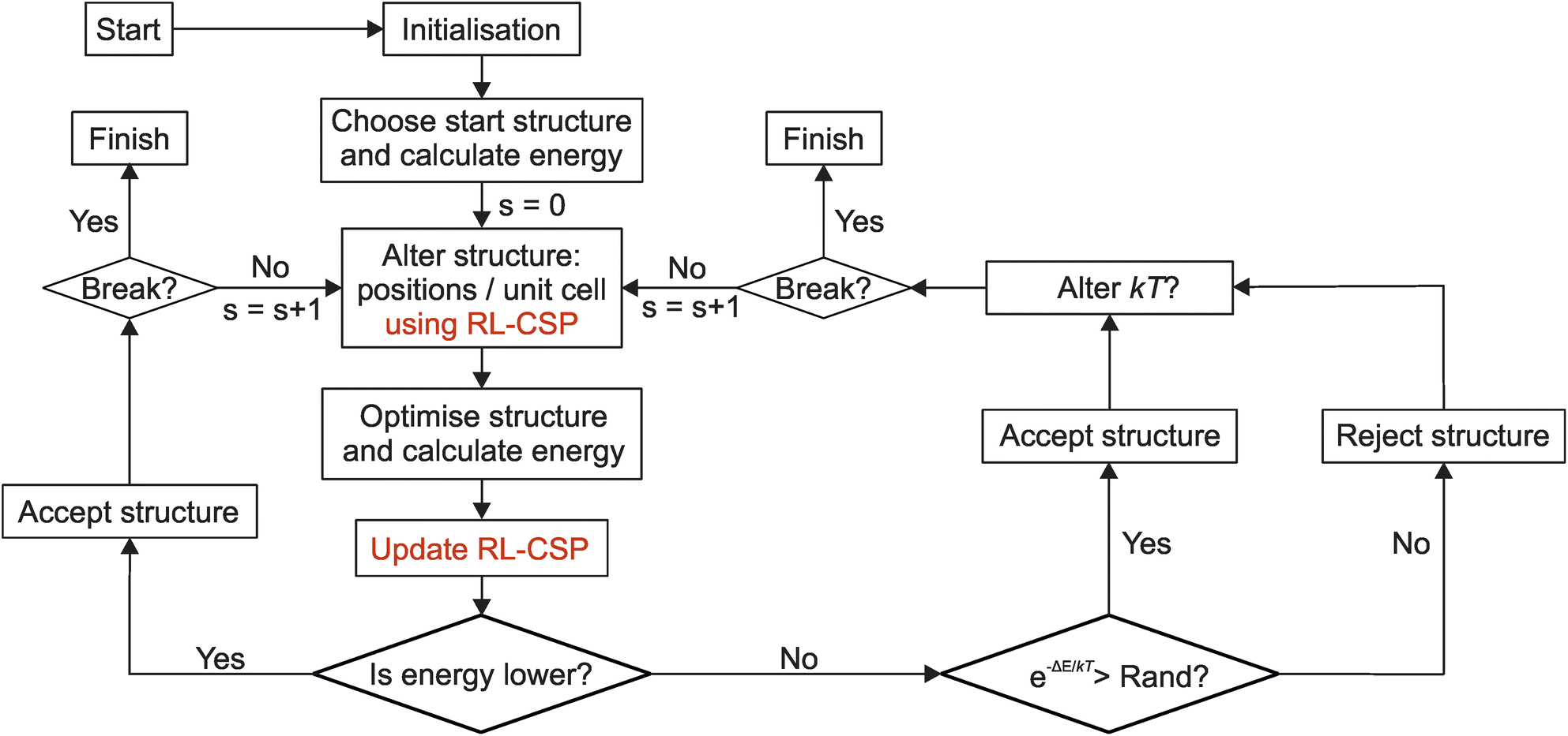

Fig. 3 Basin-hopping (BH) search routine with RL-CSP. BH (in black colour) is the basis for the searches used in both the FUSE and MC-EMMA structure prediction codes (described in ESI Notes 3 and 4†). “Rand” is a randomly generated number between 0 and 1, ΔE indicates the difference in energy between the trial structure and the current structure, kT is the “temperature” parameter for the system (set by the user). The “Break” condition is triggered when the maximum allowable number of consecutive rejected structures is reached (defined by user). The text in red shows how RL-CSP is embedded into BH; the RL-CSP policy is used instead of the fixed probability distribution to select the action to alter the structure that maximises the reward and then the policy is updated based on the results of the energy calculation.

3 Results

We measure the success of the RL approach applied to the particular CSP code by the number of steps required to locate the global minimum, given the composition. Each step involves modifying the current structure with an action followed by the local relaxation of the resulting structure. Indeed, the local relaxation of the trial structure is the most resource intensive operation during a CSP run, so we aim to reduce the number of relaxed structures, i.e., the number of steps needed to achieve the global minimum. For individual experiments, we find that the RL approach is often considerably better than the fixed policies presented here.

A common practical use case of CSP in material discovery is to identify candidate new compositions for synthesis. This amounts to approximation of the convex hull by means of CSP calculations over a wide range of compositions in the phase field.^3,26,29 As a measure of potential gain in this context, we aggregate performance improvement across all compositions within the same phase field to demonstrate that our RL implementation with FUSE outperforms the two fixed policies it is compared with, requiring less than 68% and 54% of the steps required by the fixed policies without the additional cost of having to manually tune a fixed policy.

3.1 RL-CSP in FUSE

FUSE is a CSP code designed to assemble crystal structures of ionic solids from layers (defined as modules), which are themselves constructed from small blocks (sub-modules, containing up to four atoms) generated basing on chemical knowledge. Modules are then assembled into full crystal structures by stacking them according to the rules based on either cubic or hexagonal packing (depending on the specific unit cell). FUSE has a range of nine possible actions (Fig. 4) that it can use to modify a crystal structure during the BH search, varying in impact from local actions (swapping the position of two individual atoms or sub-modules) to a global action (randomly generating a new structure); the actions are chosen independently according to a fixed user-defined probability distribution; a detailed description is presented in ESI Note 3.†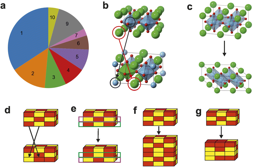

Fig. 4 Actions in FUSE. (a) The probability distribution of actions 1–7, 9–10, utilized in the FUSE study.⁴ Action 8, which is currently in development, is not used in this study. (b) Actions 1, 9 & 10 swap the positions of two, three to N − 1 or all of the atoms in the structure respectively (N is total number of atoms in the structure); these actions were labelled by number 1 in the FUSE study but the proportions they were called in match the segments in the pie chart. (c) Action 3 alters the instructions used to assemble the structure, for example by changing one of the unit cell angles. (d) Action 2 switches the positions of two sub-modules within the structure. (e) Action 4 switches the positions of two complete modules within the structure. (f) Action 5 doubles the structure along a chosen unit cell axis. (g) Actions 6 & 7 generate a new random structure. For action 6, the unit cell is limited to be of the same size or smaller, for 7 it can be of any size, so long as it conforms to the limit of the number of atoms used within a run of FUSE.

FUSE was benchmarked on compositions from the Y³⁺–Sr²⁺–Ti⁴⁺–O²⁻ phase field, containing the following known compounds: TiO₂, SrO, Sr₂TiO₄, Sr₃Ti₂O₇, SrTiO₃, Sr₄Ti₃O₁₀, Y₂TiO₅, Y₂Ti₂O₇, SrY₂O₄, Y₂O₃ (other compounds are reported, but adopt modified versions of the structures of these ten compounds).⁴ In preliminary testing, we found that TiO₂, SrO, Sr₂TiO₄, Sr₃Ti₂O₇, and SrTiO₃ are trivial for FUSE with the global minimum being found within ten BH steps, and so do not use these compositions in our experiments. We test RL-CSP integrated into FUSE on the remaining five compositions Sr₄Ti₃O₁₀, Y₂TiO₅, Y₂Ti₂O₇, SrY₂O₄, Y₂O₃, for which highly probable global minimum structures were reported.⁴ For the compositions: Sr₄Ti₃O₁₀, Y₂TiO₅, Y₂Ti₂O₇, SrY₂O₄, we allow FUSE to use up to 50 atoms per unit cell and for Y₂O₃ we allow 80, ensuring that for each composition it is possible to generate the observed global minimum structure. We contrast these results with those obtained with FUSE using two fixed policies.

In the first fixed policy, all possible actions are chosen with equal probability (Uniform). The other fixed policy was hand-tuned in the FUSE study⁴ in such a manner that the code efficiently locates the crystal structure of Y₂Ti₂O₇ with a limit of 150 atoms per unit cell. This policy is the default search policy in the FUSE code (Original, Fig. 4a). Thus the comparison of three policies, Uniform, Original and the dynamic RL-CSP policy (RL-CSP) is made by computing the structures of materials from the Y³⁺–Sr²⁺–Ti⁴⁺–O²⁻ phase field defined above.

For the test set of five compositions (Sr₄Ti₃O₁₀, Y₂TiO₅, Y₂Ti₂O₇, SrY₂O₄ and Y₂O₃), we compare performance on one key metric: the number of steps taken to identify the global minimum for each composition-policy pair (see ESI Note 5†), where each step consists of the structure modification via an action and subsequent local energy minimisation using GULP. Each step in the CSP run is followed by an accept/reject stage to determine whether to accept the new structure or retain the previous one (see Section 2.2). As CSP codes are stochastic, multiple repeat runs are required to build up statistics. While there is no common standard for how many repeat calculations to perform when testing a CSP code, typical benchmarking examples perform ∼30–70⁵, in this work we perform 40 repeats for every composition and policy tested, for a total of 600 runs across the five compositions and calculate the “mean number of steps” N_mean for each composition-policy pair. N_mean represents how many steps FUSE needs on average to find the structure with the global minimum energy (Fig. 5a and b). For the majority of compositions, namely Sr₄Ti₃O₁₀, Y₂TiO₅, Y₂Ti₂O₇, SrY₂O₄, N_mean is calculated as the mean number of steps required to find the global minimum among all 40 runs. However, the Original policy is unable to attain the global minimum for SrY₂O₄ in 28 runs out of 40, given a minimum of 90 000 steps in the search, so the lower bound on N_mean is provided for this composition-policy pair calculated as the mean number of steps to completion among 12 successful and 28 stopped runs.

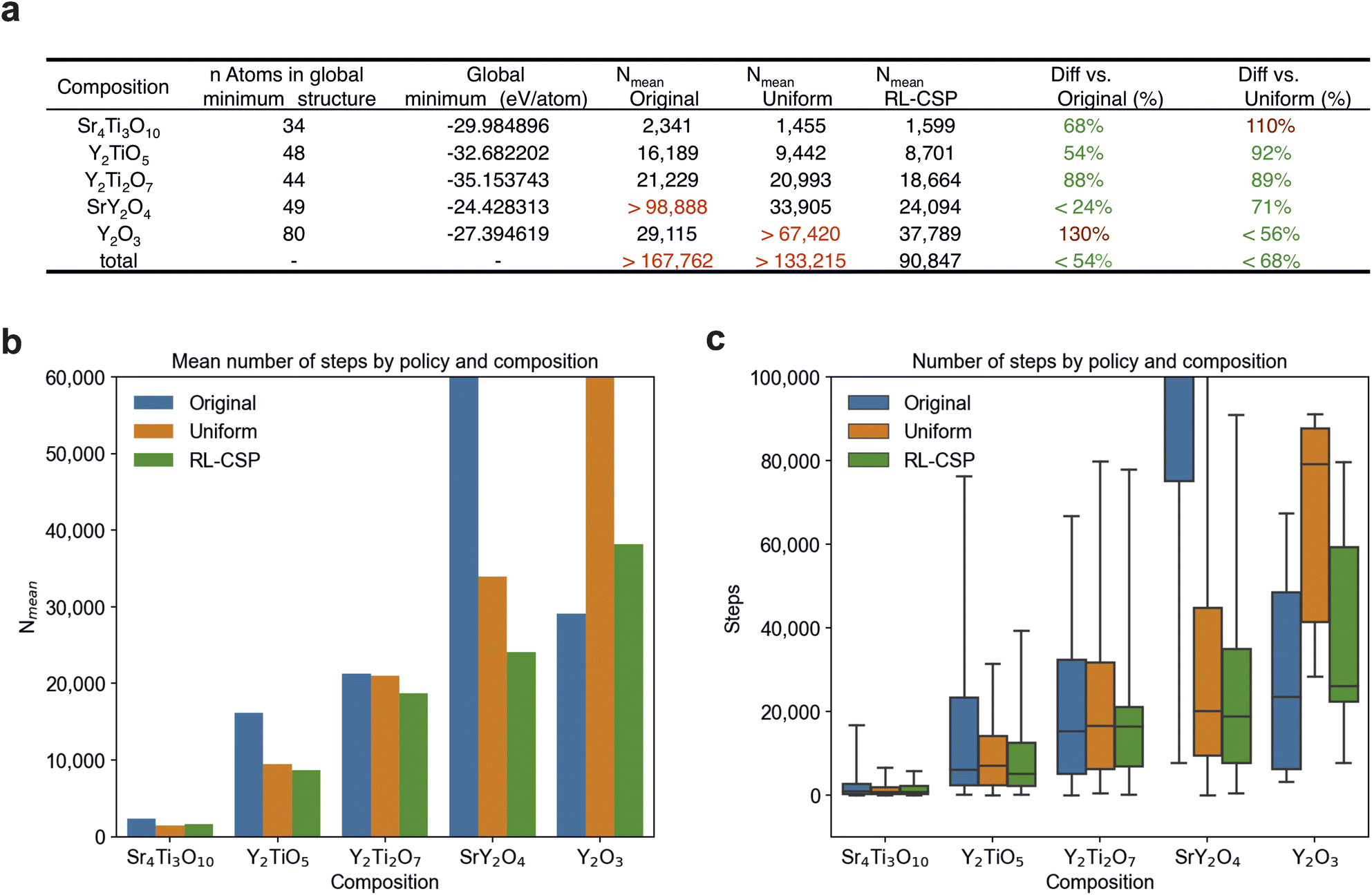Fig. 5 Number of steps required to find the global minimum for FUSE. (a) Average number of steps (N_mean) by policy and composition. For all compositions except Y₂O₃N_mean is the mean number of steps among 40 runs FUSE takes to find the global minimum. For Y₂O₃N_mean is calculated as the mean number of steps among the fastest 12 of 40 runs. For two composition-policy pairs (SrY₂O₄ with Original and Y₂O₃ with Uniform), only the lower bound is provided since the global minimum was not found in all 40 (12 fastest for Y₂O₃) runs of FUSE. The sum of steps taken for all compositions is shown in the bottom row with the lower bound for the Original and Uniform policies. The percentages given in the last two columns are the mean number of steps for the policy RL-CSP compared against Original and Uniform policies. Percentages are highlighted in green and red when RL-CSP uses fewer or more steps respectively than the policy with which it is being compared. All numbers are rounded to the nearest integer. (b) Displays the numbers from (a). (c) The number of steps required to find the global minimum structure, arranged by policy and composition. A box contains the numbers between the first and third quartiles of the data separated by the median, the maximum and minimum numbers of steps are the highest and lowest ticks (“whiskers”) respectively. Given a composition, the green (RL-CSP) box is typically shorter and placed lower than orange (Uniform) reflecting the advantage of RL-CSP over the Uniform policy that it starts with.

For Y₂O₃, the calculation of the mean number of steps required to find the global minimum among all 40 runs presents a challenge as only 12 runs on average attain the global minimum within ∼90 000 steps, with 15, 9 and 12 successful runs for Original, Uniform and RL-CSP policies respectively. As we aim to evaluate RL-CSP policy and only the steps taken to obtain the global minimum are relevant here, we use the fastest 12 runs to compute N_mean for Y₂O₃. The Uniform policy managed to find the global minimum in only 9 runs, so the mean number of steps among the 9 successful and the 3 fastest unsuccessful runs is used as the lower bound of N_mean in this case. N_mean for all composition-policy pairs is shown in Fig. 5a and coloured red if the lower bound is presented. We also display the number of steps as a distribution for each composition and policy in a box and whisker plot (Fig. 5c).

For the compositions comparing RL-CSP, Uniform and Original policies, Fig. 5 shows that RL-CSP is fastest to locate the global minimum for three compositions (Y₂TiO₅, Y₂Ti₂O₇ and SrY₂O₄), and the second fastest for two; Sr₄Ti₃O₁₀ behind Uniform and Y₂O₃ behind Original. The latter case is discussed in detail in the subsequent section, the analysis of the former case reveals that although RL-CSP does not improve upon the Uniform policy for Sr₄Ti₃O₁₀, the difference between their N_mean (144 steps) is relatively small. Thus, we conclude that the efficiency of RL-CSP is comparable to that of Uniform, and that the lack of improvement from learning in Sr₄Ti₃O₁₀ can be attributed to the limited duration of the runs in this case.

We also provide a comparison based on N_mean for all five compositions, which represents the average number of steps taken across 40 runs for each of Sr₄Ti₃O₁₀, Y₂TiO₅, Y₂Ti₂O₇, and SrY₂O₄, along with the 12 fastest runs for Y₂O₃, resulting in a total of 172 runs. When compared with either fixed policy, RL-CSP is faster over the whole test set of compositions within the phase field, as judged by N_mean for all of the compositions, using fewer than 68% and 54% of the steps required by the Uniform and Original fixed policies respectively (Fig. 5a). The effect of learning across the phase field is more pronounced for more challenging compositions (for the Uniform policy) based on the strictly decreasing numbers in the last column of Fig. 5a. This leads to improved absolute savings of computational resources for the compositions for which they matter the most.

3.2 Comparison of RL-CSP with fixed policies for SrY₂O₄ and Y₂O₃

In this section we examine in detail the two compositions that best demonstrate the benefits of RL over a fixed policy, SrY₂O₄ and Y₂O₃ (Fig. 6). With Y₂O₃, the fixed Original policy is the most efficient of the three approaches. However, as Uniform is 2.3 times slower than the Original policy, RL-CSP does need time to optimize it (recall that RL-CSP begins with the Uniform policy) and reach the performance of Original. RL-CSP improves the starting policy significantly as its successful 12 runs took at most 56% of the steps required by Uniform. We observe that RL-CSP learns an efficient policy. Fig. 6d illustrates that after the first ∼30 000 steps approximately the same number of runs of RL-CSP have found the global minimum as those of Original, demonstrating the ability of RL to reproduce the efficiency of the well-tuned policy despite starting from a clearly unsuited policy. By the end of the runs, RL-CSP closes the gap, being only 1.3 times slower than Original (Fig. 5a).

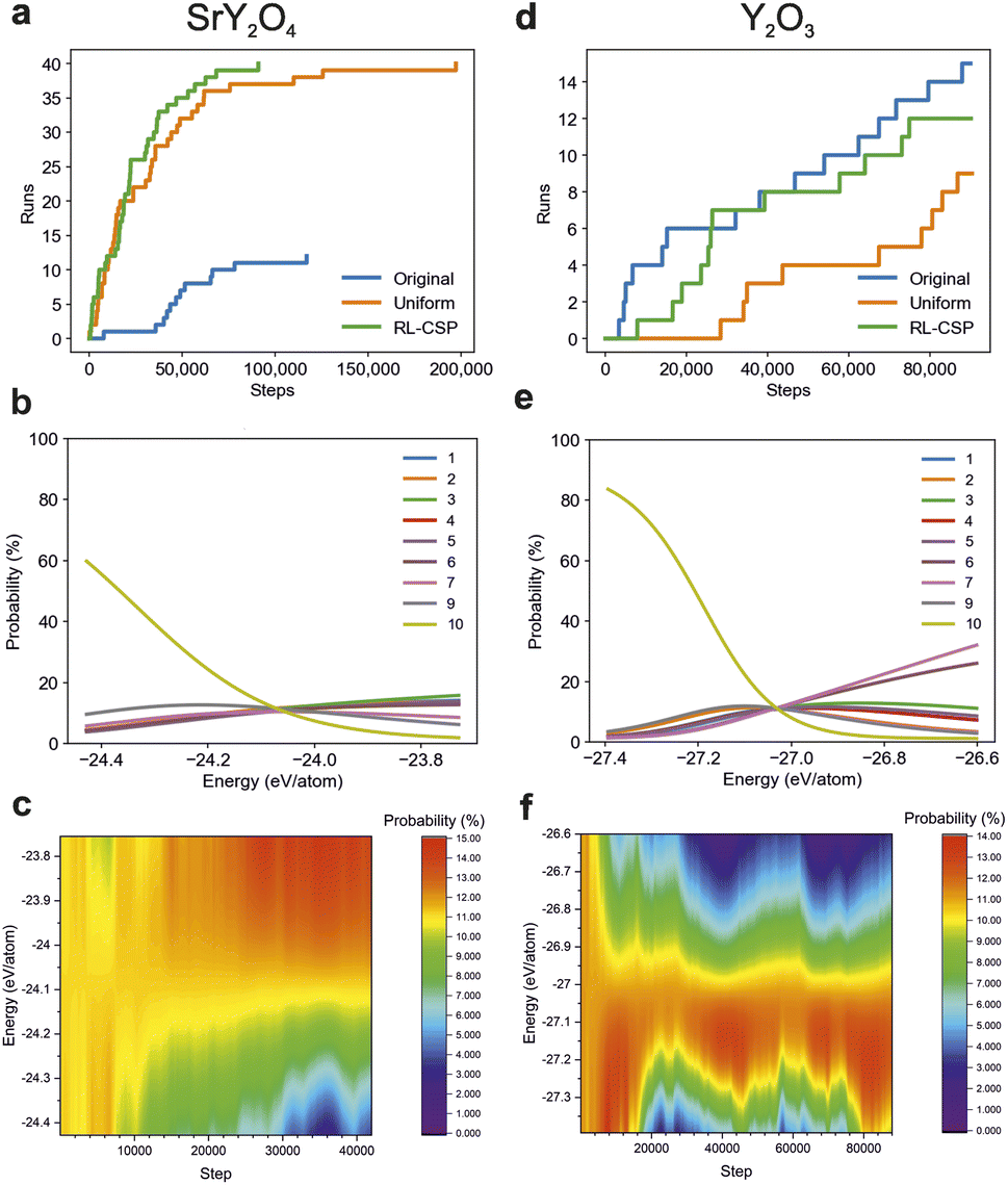Fig. 6 Efficiency of different FUSE policies at the compositions SrY₂O₄ and Y₂O₃. (a) and (d) show how many runs have found the global minimum in the given number of steps. The analogous plots for compositions Sr₄Ti₃O₁₀, Y₂TiO₅, Y₂Ti₂O₇ are provided in ESI Fig. 1(a–c).† (b and e) show the final policies learnt by RL-CSP for SrY₂O₄ (b) and Y₂O₃ (e) at the end of a typical RL-CSP run. (b and e) confirm that, unlike the fixed policy (see Fig. 4a) RL-CSP policy provides an action probability distribution that depends on the composition and the energy of the current structure. The typical final policies for Sr₄Ti₃O₁₀, Y₂TiO₅, Y₂Ti₂O₇ are presented in ESI Fig. 1(d–f)† respectively. (c and f) show the full dynamic policy for action type 2 (swap the position of two sub-modules within the structure), varying with both energy (the full energy range found for both compositions are shown) and step number for SrY₂O₄ and Y₂O₃ respectively, illustrating that for different compositions, RL-CSP uses very different policies for the same action type between compositions.

In contrast to Y₂O₃, for SrY₂O₄ the Uniform policy is the best of the two fixed policies, being at least 2.9 times faster than Original. RL-CSP is then able to learn a policy that improves upon the performance of the Uniform policy (Fig. 6a), resulting in a significantly further reduced N_mean with RL-CSP using just 71% of the steps required by Uniform.

These cases show that a fixed policy, even when tuned by hand, can demonstrate particularly poor performance for some compositions, for example, in the original FUSE study⁴ the global minimum for SrY₂O₄ was not obtained. In this work, the Uniform policy for Y₂O₃ and the Original policy for SrY₂O₄ both have a low success rate at finding their respective energy minima. The dynamic RL-CSP policy reliably improves the Uniform starting policy for both materials, taking at most 56–71% of steps required by the initial fixed policy.

Finally, we observe a clear improvement in the dynamic policies used by RL-CSP during a CSP run, illustrated by plotting the probability of RL-CSP using action 2 (swapping the position of two sub-modules) with both the step number and energy (Fig. 6c and f). Studying the dynamic policy for different compositions illustrates that the learned policy not only depends on the composition, but also on the structure that the CSP run is currently located in, as in no cases does RL-CSP converge to an ideal probability distribution that works best for all structures at a given composition. However, for both compositions action 10 (Fig. 4b) exhibits a greater preference in lower energy structures, indicating its increasing significance at low energy levels (Fig. 6b and e).

The comparison of RL-CSP performance in SrY₂O₄ and Y₂O₃ with different fixed policies indicates that, while manually tuned fixed policies may be able to provide a performance advantage over RL-CSP for specific compositions, such as the Original policy for Y₂O₃, RL-CSP should be the default option when exploring a whole phase field because this necessitates performing CSP for a range of compositions, and RL tailors the policy dynamically to each composition, thus avoiding locked-in poor performance from a fixed policy, such as the Original policy for SrY₂O₄ or the Uniform policy for Y₂O₃.

3.3 RL-CSP in MC-EMMA

In order to demonstrate the more general applicability of RL in the context of CSP, the study was expanded to include another CSP code MC-EMMA.²⁶ The original EMMA code was designed to identify the crystal structures of oxides by assembly of layered units, and was crucial in the structure determination of the phase Y_2.24Ba_2.28Ca_3.48Fe_7.44Cu_0.56O₂₁,³⁰ with a subsequent version with implementing a BH search (MC-EMMA) used to identify Y_0.07Sr_1.01Ca_1.55Ga_2.87O₇ and Y_0.038Sr_0.32Ca_0.848Ga_0.794O_2.416 in the Y–Sr–Ca–Ga–O phase field,²⁶ and so the code is established and well developed.

MC-EMMA uses a BH routine that is similar to FUSE, however it was designed for larger crystal structures with up to 160 atoms while FUSE was tested with the structures up to 50–80 atoms depending on the composition. Although fewer steps are usually required to find the global minimum (∼1500–2000 steps for fixed policies) than those in most FUSE compositions, the relaxation of the larger structures is more time-consuming and so MC-EMMA presents a different challenge for RL, which is to improve the starting policy using less data. As in the evaluation of RL for FUSE, we compare three versions of policy in MC-EMMA: the original hand-tuned fixed policy (Original), the uniform policy (Uniform) and the RL-CSP policy that starts learning from the Uniform. The action probability distributions for the Original policy are shown in ESI Fig. 2a.† We test MC-EMMA policies at the composition YBa₂Ca₂Fe₅O₁₃, which the Original policy was tuned for. As in the FUSE benchmarking, we use 40 runs of MC-EMMA with each policy. However, in FUSE we observed that RL-CSP does not have enough time to learn the policy at compositions where N_mean is less than ∼10 000 steps for the Uniform policy (Sr₄Ti₃O₁₀ and Y₂TiO₅). Taking this into account, we boost the learning process in RL-CSP by increasing the learning rate to 0.01 (see Section 2.1) in comparison to the FUSE settings and sharing the policy learning process across 40 runs.

The policy sharing is organised via the policy vector θ, which is common for all runs. 40 runs start simultaneously but choose the initial structure independently. Each run follows its own trajectory (sequence of structures and actions) and does not consider the trajectories of other runs. Given the current structure, a run selects an action according to the shared policy θ, observes a new structure and utilizes the obtained reward to update θ. When the run finds the global minimum, it stops while other working runs continue following their own trajectories in which they did not find the global minimum yet. Fig. 7e demonstrates the shared policy learned by 40 runs of MC-EMMA with RL-CSP.

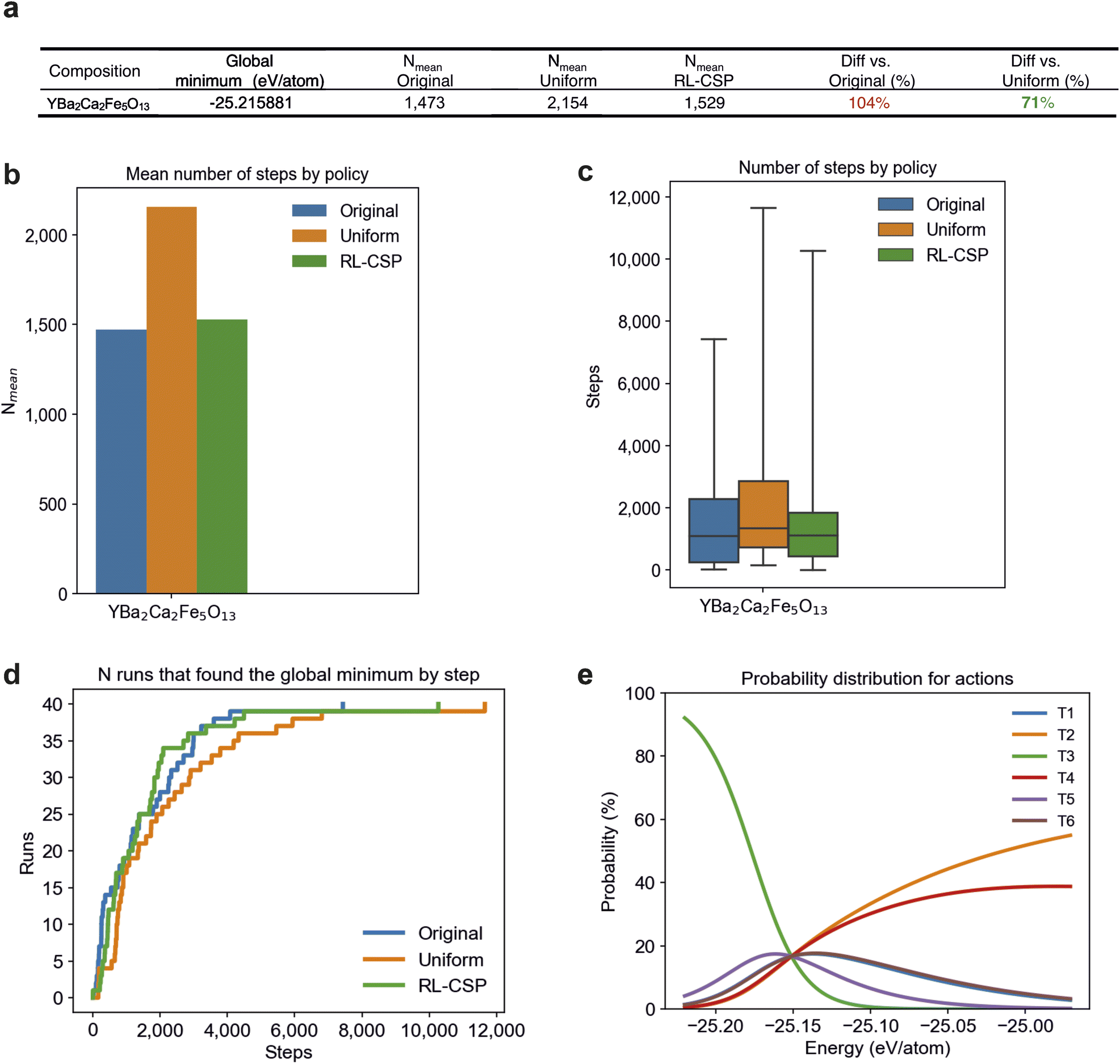Fig. 7 Number of steps required to find the global minimum for MC-EMMA. (a) Average number of steps (N_mean) among 40 runs MC-EMMA requires to find the global minimum by policy. The Original policy performs best while RL-CSP shows a similar performance, with only 4% more steps on average. RL-CSP improves the starting Uniform policy requiring only 71% steps of those by Uniform. The percentages given in the last column are as a percentage of the moves used in the policy RL-CSP is being compared against. Percentages are highlighted in green and red when RL-CSP uses fewer or more steps respectively than the policy with which it is being compared. (b) Displays the numbers from (a). (c) The number of steps required to find the global minimum structure, arranged by policies. (d) shows the number of runs that found the global minimum on the given step by polices. (e) shows the shared learned policy after 40 runs finished. The policy depends on the energy of the current structure, favouring action T3 in the low energy structures and T2 and T4 in the high energy structures.

We compare the performances of different policies using N_mean; the mean number of steps required to find the global minimum among 40 runs (Fig. 7). The numbers in Fig. 7a show clear RL-CSP improvement over the starting policy, as it uses only 71% of the steps required by Uniform to find the global minimum. Due to learning sharing between runs, the RL-CSP policy (Fig. 7e) can be efficiently learned even though the average number of steps per run is relatively small (∼1500). Finally, RL-CSP essentially reproduces the performance of the Original policy, requiring just 4% more steps despite starting from Uniform.

4 Conclusion

The implementation of reinforcement learning via the policy gradient algorithm was compared with two fixed policies in two basin-hopping CSP codes with six tested compositions overall. The results showed improvement over an initial uniform policy for five of the six compositions and over a hand-tuned policy for four of the six. As RL-CSP adds only minimal computational cost since it learns on the fly using available data, we conclude that it improves basin-hopping CSP at essentially no extra cost. The RL-CSP code is available on GitHub (https://github.com/lrcfmd/rlcsp) and can be readily applied to other CSP algorithms.

Considering the specific practical case of calculating the convex hull for a phase field to identify candidate new compositions for synthesis, the ability of reinforcement learning to improve a fixed policy enables the development of policies tailored to each composition within the phase field and should favour the more rapid construction of the hull. Although it is possible that a single fixed policy performs best at the some of the compositions studied, this study indicates that this is not likely to be the case in general, favouring further development of RL in CSP. Specifically, autonomous exploration across compositions of a phase field can benefit from RL, as our work suggests at least 32% improvement of RL-CSP when compared with the starting uniform policy.

Many such developments can be envisaged, for example in the type of reinforcement learning algorithm that could be applied beyond policy gradient methods. The learning model in RL-CSP operates only with energy as a feature to define the state space. This simplicity allows efficient operation. However, enriching the feature space with relevant structural characteristics would make learning quicker and more accurate. For this purpose, one could implement known structural characteristics such as the bond valence sum, or deploy neural networks to reveal the most relevant structural features, such as characteristic local coordination geometries for specific elements. More advanced RL algorithms can be adapted to the basin-hopping routine, for example, actor-critic methods were developed to deal with the high variance often encountered in policy gradient methods.^31–33 In non-basin-hopping CSP algorithms containing decisions that constitute a policy, these decisions could also be amenable to reinforcement learning optimisation.

Data availability

The numbers of steps in algorithms which were used to calculate N_mean are placed in ESI Tables 1 and 2† and their detailed interpretation is provided in ESI Note 2.† Input files used to produce the reported results are provided in the code repositories.

Code availability

The source codes implemented and/or used in this study are available on the following GitHub repositories: https://github.com/lrcfmd/rlcsp (RL-CSP code), https://github.com/lrcfmd/FUSE_RL (FUSE with RL-CSP), https://github.com/lrcfmd/FUSE-stable (FUSE with the fixed policy), https://github.com/lrcfmd/MC-EMMA-RL (MC-EMMA with RL-CSP), https://github.com/lrcfmd/MC-EMMA-stable (MC-EMMA with the fixed policy).

Author contributions

All authors considered the application of ML to CSP. E. Z. designed the exact RL approach and implemented the code, with contributions from R. S., V. V. G. and C. M. C. E. Z. performed computational experiments with assistance from C. M. C. and D. A. All authors contributed to the experiments results analysis and discussion. E. Z. wrote the first draft with contributions from V. V. G., C. M. C., D. A. and M. J. R. E. Z., C. M. C., V. V. G., R. S. and D. A. wrote the final manuscript with contributions from M. D. and P. G. S. All authors read and approved the final manuscript. R. S. and M. J. R. directed the research.

Conflicts of interest

There are no conflicts to declare.

Acknowledgements

The authors acknowledge funding from the Leverhulme Trust via the Leverhulme Research Centre for Functional Materials Design. For the purpose of open access, the authors have applied a Creative Commons Attribution (CC BY) licence to any Author Accepted Manuscript version arising from this submission.

References

1. S. M. Woodley and R. Catlow, Nat. Mater., 2008, 7, 937–946.
2. J. Yang, S. De, J. E. Campbell, S. Li, M. Ceriotti and G. M. Day, Chem. Mater., 2018, 30, 4361–4371.
3. A. R. Oganov, C. J. Pickard, Q. Zhu and R. J. Needs, Nat. Rev. Mater., 2019, 4, 331–348.
4. C. M. Collins, G. R. Darling and M. J. Rosseinsky, Faraday Discuss., 2018, 211, 117–131.
5. A. O. Lyakhov, A. R. Oganov, H. T. Stokes and Q. Zhu, Comput. Phys. Commun., 2013, 184, 1172–1182.
6. Q. Tong, J. Lv, P. Gao and Y. Wang, Chin. Phys. B, 2019, 28, 106105.
7. C. J. Pickard and R. J. Needs, J. Phys.: Condens. Matter, 2011, 23, 053201.
8. P. V. Bushlanov, V. A. Blatov and A. R. Oganov, Comput. Phys. Commun., 2019, 236, 1–7.
9. S. Manna, T. D. Loeffler, R. Batra, S. Banik, H. Chan, B. Varughese, K. Sasikumar, M. Sternberg, T. Peterka, M. J. Cherukara, S. K. Gray, B. G. Sumpter and S. Sankaranarayanan, Nat. Commun., 2022, 13, 368.
10. S. Gow, M. Niranjan, S. Kanza and J. G. Frey, Digital Discovery, 2022, 1, 551–567.
11. G. Czibula, M. Bocicor and I.-G. Czibula, Int. J. Comput. Appl. Technol., 2011, 2.
12. K. Ahuja, W. H. Green and Y.-P. Li, J. Chem. Theory Comput., 2021, 17, 818–825.
13. M. H. Segler, M. Preuss and M. P. Waller, Nature, 2018, 555, 604–610.
14. Z. Zhou, X. Li and R. N. Zare, ACS Cent. Sci., 2017, 3, 1337–1344.
15. D. J. Wales and J. P. Doye, J. Phys. Chem. A, 1997, 101, 5111–5116.
16. S. Yang and G. M. Day, J. Chem. Theory Comput., 2021, 17, 1988–1999.
17. C. J. Burnham and N. J. English, J. Chem. Theory Comput., 2019, 15, 3889–3900.
18. A. Banerjee, D. Jasrasaria, S. P. Niblett and D. J. Wales, J. Phys. Chem. A, 2021, 125, 3776–3784.
19. M. L. Puterman, Markov decision processes: discrete stochastic dynamic programming, John Wiley & Sons, 2014.
20. R. J. Williams, Mach. Learn., 1992, 8, 229–256.
21. R. S. Sutton and A. G. Barto, Reinforcement learning: An introduction, MIT press, 2018.
22. H. S. Obaid, S. A. Dheyab and S. S. Sabry, 2019 9th Annual Information Technology, Electromechanical Engineering and Microelectronics Conference, IEMECON, 2019.
23. A. Y. Ng, D. Harada and S. Russell, Proceedings of the 16th International Conference on Machine Learning, 1999.
24. C. Banerjee, Z. Chen and N. Noman, arXiv, 2022, preprint, arXiv: 2210.00211,  DOI:10.48550/arXiv.2210.00211.
25. Z. Ahmed, N. Le Roux, M. Norouzi and D. Schuurmans, Proceedings of the 36th International Conference on Machine Learning, 2019.
26. C. M. Collins, M. S. Dyer, M. J. Pitcher, G. F. S. Whitehead, M. Zanella, P. Mandal, J. B. Claridge, G. R. Darling and M. J. Rosseinsky, Nature, 2017, 546, 280–284.
27. C. M. Collins, L. M. Daniels, Q. Gibson, M. W. Gaultois, M. Moran, R. Feetham, M. J. Pitcher, M. S. Dyer, C. Delacotte and M. Zanella, Angew. Chem., Int. Ed., 2021, 60, 16457–16465.
28. J. D. Gale and A. L. Rohl, Mol. Simul., 2003, 29, 291–341.
29. A. R. Oganov, Y. Ma, A. O. Lyakhov, M. Valle and C. Gatti, Rev. Mineral. Geochem., 2010, 71, 271–298.
30. M. S. Dyer, C. M. Collins, D. Hodgeman, P. A. Chater, A. Demont, S. Romani, R. Sayers, M. F. Thomas, J. B. Claridge and G. R. Darling, Science, 2013, 340, 847–852.
31. V. Mnih, A. P. Badia, M. Mirza, A. Graves, T. Lillicrap, T. Harley, D. Silver and K. Kavukcuoglu, Proceedings of The 33rd International Conference on Machine Learning, 2016.
32. J. Schulman, F. Wolski, P. Dhariwal, A. Radford and O. Klimov, arXiv, 2017, preprint, arXiv: 1707.06347,  DOI:10.48550/arXiv.1707.06347.
33. M. Sewak, Deep reinforcement learning, Springer, 2019.

---

Footnote

† Electronic supplementary information (ESI) available. See DOI: https://doi.org/10.1039/d3dd00063j

---