Spinel nitride solid solutions: charting properties in the configurational space with explainable machine learning

Abstract

Ab initio prediction of the variation of properties in the configurational space of solid solutions is computationally very demanding. We present an approach to accelerate these predictions via a combination of density functional theory and machine learning, using the cubic spinel nitride GeSn₂N₄ as a case study, exploring how formation energy and electronic bandgap are affected by configurational variations. Furthermore, we demonstrate the utility of applying explainable machine learning to understand the crystal chemistry origins of the trends that we observe. Different configuration descriptors (Coulomb matrix eigenspectrum, many-body tensor representation, and cluster correlation function vectors) are combined with different models (linear regression, gradient-boosted decision trees, and multi-layer perceptron) to extrapolate the calculation of ab initio properties from a small set of configurations to the full space with thousands of configurations. We discuss the performance of different descriptors and models. SHAP (SHapley Additive exPlanations) analysis of the machine learning models highlights how values of formation energy are dominated by variations in local crystal structure (single polyhedral environments), while values of electronic bandgap are dominated by variations in more extended structural motifs. Finally, we demonstrate the usefulness of this approach by constructing structure–property maps, identifying important configurations of GeSn₂N₄ with extremal properties, as well as by calculating accurate equilibrium properties using configurational averaging.

---

1. Introduction

Computational methods play a major role in the exploration of the configurational space of solid solutions. Density functional theory (DFT)^1,2 is the most extensively used materials simulation technique at electronic-level, because of its accuracy and relatively modest computational cost compared to other methodologies. However, the application of DFT simulations to evaluate the properties of the huge number of configurations of ion distributions in alloys is still a formidable task. In recent years, machine learning (ML) is attracting a lot of attention due to its capability to drastically accelerate materials simulations and reduce its cost by several orders of magnitude, acting as a surrogate model by using the results obtained from DFT programs.^3–9 A common criticism of ML approaches is that they represent black-box answers providing little physical insight, however recent work in explainable machine learning (commonly called XAI) shows the potential to extract meaningful explanations from complex ML models.^10,11,65 Herein we demonstrate the application of DFT combined with ML and XAI to exploring the configurational space of a prototypical mixed cation spinel material.

Silicon nitride, Si₃N₄, a wide bandgap ceramic with very high abrasion and oxidation resistance,^12,13 is one of the most commonly used 3 : 4 nitrides in industry. Si₃N₄ can form different polymorphs, with the hexagonal α and β phases being the most energetically favorable ones. Advances in high-pressure and temperature synthesis methods have led to the discovery of the novel spinel (cubic) γ-phase of Si₃N₄ and analogous structures for a range of different cations, specially group 14.¹⁴ This family of compounds possesses a promising combination of the properties of the more stable phases, plus outstanding mechanical features, with impressive hardness values,¹⁵ and great tunability of their electronic properties.¹⁶ Spinel phases of Sn₃N₄ and Ge₃N₄, with reduced bandgap values (1.6 eV and 3.5 eV, respectively),¹⁷ in comparison with their respective α- and β-phases, are stable semiconductors with large exciton binding energies and electron mobilities.¹⁸ This set of properties opens the door for new applications beyond coatings and mechanical applications, for example, in light emitting diodes, photocatalysis, sensors or electrodes for batteries.^17–20 Additionally, a recent study pointed to spinel compounds, with their uncommon structure with mixed tetrahedral and octahedral bonding, as potential candidates to substitute conventional absorber materials in solar cells, offering a good compromise between typical high defect tolerance and long-term stability of tetrahedral and octahedral systems respectively.²¹

ML has made a considerable impact on the field of alloy and solid-solution materials design. Given the complex, high-dimensional search spaces, methods that can accelerate predictions and guide and inform choice of experiments are particularly promising. ML has been used to develop accurate, but computationally efficient interatomic potentials, that can be applied for calculating phase diagrams,²² and for exploring high-entropy alloys.²³ ML has also been used, for example to explore the binding energies at the surfaces of alloy catalysts, a task that would be too computationally demanding using first principles approaches.²⁴ We previously demonstrated how ML could be used to predict band gaps and formation energies for arbitrary configurations of the ionic solid solution (Mg,Zn)O.³ ML approaches are also extremely useful for guiding experimental studies and have been used for example to fuse experiment and theory for optimization of a halide perovskite solid-solution to optimize stability²⁵ and to discover optimal phase change memory materials in a complex composition/processing space.²⁶

The present work explores Sn/Ge nitride solid solutions, which have been theoretically predicted to have favourable electronic properties for use in high-efficiency solar cells, such as tandem or intermediate-band solar cells.²⁷ Here, instead of attempting to engineer the properties of the solid solution via changes in composition, as done by Hart et al. for ternary Si/Ge nitrides,²⁸ we investigate how properties change as a function of the distribution of cations in a single composition, GeSn₂N₄. This is in spirit of growing theoretical and experimental work that has demonstrated that controlling the ion distribution is a viable route to tune the physical properties and functional behavior of materials.^29–33 In this work, we use a combination of DFT and ML techniques to investigate the properties of the GeSn₂N₄ solid solution as a function of cation distribution configuration. We focus on the mixing energies E_mix, and the electronic bandgaps E_g. Supervised learning of these properties, from DFT results obtained for a small fraction of the total number of configurations, allows their accelerated prediction for the full configurational space. We test different combinations of descriptors and models, with the goal of developing a methodology that allows us to perform a computationally efficient investigation of the properties of these spinel nitrides, and progress towards their optimization for photovoltaic applications. We then use the SHAP³⁴ (SHapley Additive exPlanations) approach to extract physical interpretations from our model predictions, linking observed changes in formation energy and bandgap to specific crystal chemistry motifs. We use our approach to construct structure–property maps that can be used to efficiently identify important and useful relationships and pick out extreme examples and can be combined to obtain ensemble averages, which highlights the potential application of processing conditions for property tuning. The methods that we present are applicable to a wide range of important problems where rational design of solid solutions is a key technological enabler.

2. Methodology

2.1 Density functional theory simulations

All the DFT calculations carried out in this work were done with the Vienna Ab initio Simulation Package (VASP),^35,36 following the projector augmented wave (PAW) formalism.³⁷ The results presented come from full structural relaxations of the different configurations, performed at a generalized-gradient approximation (GGA) level with the Perdew–Burke–Ernzerhof (PBE) functional³⁸ and convergence criteria of 10⁻⁷ eV and 10⁻² eV Å⁻¹ for total energies and forces respectively. We used Hubbard corrections for the d-orbitals of Sn and Ge, following Dudarev's approach (GGA + U),^39,40 as this correction was found to improve the agreement with experiment for the binary nitrides, in terms of both geometric and electronic structure. Different U_eff values were tested, as presented in Table S1 of the ESI,† finding best agreement for U_eff = 2 eV. For all the calculations, the plane wave kinetic energy cutoff was set to 520 eV, which is 30% higher than the suggested value for standard accuracy calculations with the given set of PAW potentials. For integration in the reciprocal space, the Brillouin zone has been sampled with a 2 × 2 × 2 k-points grid.

It is well known that the GGA generally produces underestimated bandgaps. In this work we found that the underestimation was ∼1.5 eV against experimental results for the pure binary reference compounds. The GGA + U correction, although improving over GGA, was not enough to overcome this deficit. For that reason, and trying to produce physically and experimentally meaningful results for that central property, the screened hybrid functional by Heyd–Scuseria–Ernzerhof (HSE)⁴¹ was also used for the reference binary compounds and subsequently for a subset of configurations within the calculated space. We will discuss below that a strong correlation exists between GGA + U and HSE bandgaps, which allowed us to reduce the computational cost of accurate bandgap predictions across the configurational space. Our HSE calculations, with 25% of exact exchange and a range-separation parameter of 0.2 (corresponding to the HSE06 parameterization), were single-point calculations on top of the GGA + U relaxed structures. Table 1 presents the results of lattice parameter and bandgap for the reference binary compounds and the different calculation levels.

Table 1 Calculated and experimental values of lattice constant and bandgap for the reference compounds γ-Sn₃N₄ and γ-Ge₃N₄

	Lattice constant (Å)	PBE + U bandgap (eV)	HSE bandgap (eV) (at PBE + U geometry)
γ-Sn3N4:DFT	9.05	0.62	1.66
Exp.	9.03	—	1.6 ± 0.2,^17 1.6 (ref. 18)
γ-Ge3N4:DFT	8.24	2.30	3.50
Exp.	8.21	—	3.5 ± 0.2,^17 3.65 ± 0.05 (ref. 42)

---

2.2 Cation configurations

We consider the distribution of Ge and Sn atoms in the 56-atom spinel cubic unit cell of γ-GeSn₂N₄ with Fd3m symmetry. The inversion degree of an AB₂X₄ spinel is the fraction of tetrahedral sites that is occupied by B cations. Since the number of octahedral sites is double the number of tetrahedral sites in a spinel structure, a “normal” distribution is defined as one where the A cations occupy the tetrahedral sites and the B cations occupy the octahedral sites. The concept of inversion degree has been widely used for II–III₂–VI₄ spinels, where it represents the fraction of tri-valent cations in tetrahedral positions, and for II₂–IV–VI₄ spinels, where it represents the fraction of di-valent cations in tetrahedral positions. In our case, both cations are formally tetravalent, but the concept of inversion degree remains useful as a single, scalar descriptor of the cation distribution. The inversion degree, y, of GeSn₂N₄ is defined here as the fraction of tetrahedral sites occupied by Sn cations. Thus, y = 0 refers to a normal or direct spinel, where all the Ge atoms are in tetrahedral positions, and all Sn are in octahedral positions, avoiding partial occupancy of sites; whereas y = 1 refers to a fully inverse distribution where all the tetrahedral sites are fully occupied by Sn. A representation of both structures, direct and inverse (one of the possible distributions because of the partial occupancy), is presented in Fig. 1. The formula unit can then be written as (Ge_1−ySn_y)[Sn_2−yGe_y]N₄, where the round brackets “()” represent the tetrahedral sites and the square brackets “[]” represent the octahedral sites.

Fig. 1 Structures of the direct (y = 0) and an inverse (y = 1) GeSn₂N₄ spinel. Ge: green; Sn: blue; N: gray.

The configurational space for the cell size sampled (the conventional cubic cell) has a total of 4222 symmetrically inequivalent configurations, which were generated using the SOD code, together with their degeneracies in the full configurational space.⁴³ Out of those configurations, only 1013 (24%) were calculated at DFT level, to train and test the ML models. The configurations for DFT calculations were chosen randomly and separately for each inversion degree; in that way we ensured the selection was homogeneously distributed across all the different inversion degrees within the space. For the HSE calculations, a subset of 59 configurations was selected, though in this case configurations were not chosen randomly but uniformly spaced from the lowest to the highest across the range of bandgap values. Disaggregated numbers of total and calculated configurations for each of the inversion degrees are presented in Table S2 of the ESI.†

2.3 Descriptors and models for machine learning

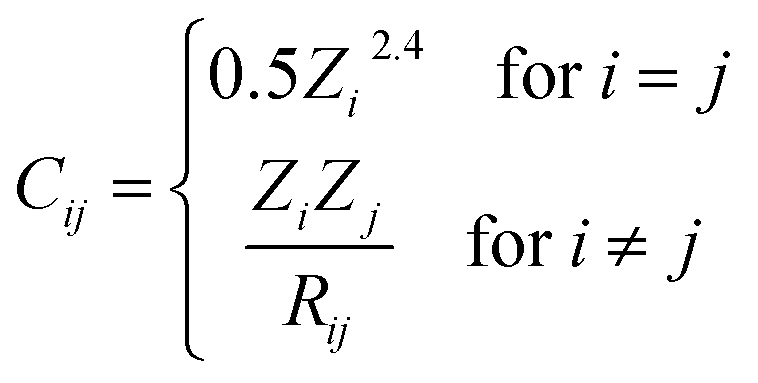
A numerical way of fully describing structures is needed to use ML or other statistical models; these numerical representations are the descriptors. These descriptors must be invariant to symmetry operations, complete and unique, meaning being able to distinguish between any two different structures.⁴⁴

Although some other descriptors like Ewald and Sine matrices⁴⁵ have also been tested in this work, only the main three descriptors for which we obtained best results are explained in detail here. None of the descriptors tested make use of periodic boundary conditions, they are calculated solely within the supercell used for the configurations. The first one is the Coulomb matrix,⁴⁶ whose elements (C_ij) represent the electrostatic interactions between the nuclei in the compound:

where Z_i is the atomic number of atom i, and R_ij is the distance between atoms i and j. For the sake of simplicity, the input for the machine learning model is not the Coulomb matrix directly, but the Coulomb matrix eigenspectrum (CME), which is the vector formed by its eigenvalues sorted by size.

The second descriptor used is the many-body tensor representation (MBTR),⁴⁷ a structure descriptor that is easily interpretable and visualised. MBTR consists of a set of values of interatomic distances and angles around which weights and broadening are added, obtaining a set of spectra:

where ω_k and D represent the weighting and the broadening applied to the element matrix C, for every function g_k considered which in our case define atom counts and inverse distances. The information represented is adjustable. For instance, dihedral angles could be included, but we have not considered them in our study, because of the extra complexity added to the descriptor, without a significant improvement in the results.

Finally, another descriptor with a long record in the prediction of solid solutions thermodynamic properties, are the cluster correlation functions (CCFs).⁴⁸ These are the basis of the cluster expansion method, although in that methodology a linear approach is used, whereas in our study we will also consider non-linear models based on the CCFs. The alloy configuration is described through the occupation of the different positions in the crystal lattice, selected in specific clusters or arrangements up to a desired order (individual atoms, pairs, trios, etc.). The CCF X_mα for a configuration m and cluster α can be defined as the average of the product of the functions ϕ_ms (which here take values of 0 and 1 depending on the atom occupying the site s in configuration m) over all the clusters of type α:

where Ω_α are the multiplicities (number of symmetrically equivalent clusters of type α in the cell). In this work, we employed the Python package CELL⁴⁹ to obtain the CCF vectors X_m = {X_mα} corresponding to clusters of up to third order for each of the 4222 symmetrically different configurations of GeSn₂N₄.

All these descriptors were used to feed different ML models, to test the performance of each descriptor–model pair, with the aim of finding the best fit for the configurational space we are investigating. Among those models we used a simple multilinear regressor (LR), including LASSO regularization⁵⁰ to constrain coefficients to physically reasonable values. Two more complex models were also trained: a gradient boosted decision trees regressor (GBDT),⁵¹ with 1000 estimators and a maximum depth of 4 nodes, and a multilayer perceptron (MLP).⁵² The MLP employed is a class of feedforward neural network, in this case with a 5-layer architecture, with 256-128-64-32-1 nodes respectively, and intermediate layers between each of those for normalization and random dropout. Rectified linear unit (ReLU) has been used as activation function for each layer except for the last one, where a linear function was needed. Squared errors were used as loss functions for all the models. More info on the parametrization and architecture of the models, which was also chosen based on a previous study,³ is presented in Table S2 of the ESI.†

To assess the performance of the different models and descriptors the main metric that has been used is the mean absolute error (MAE), although other additional metrics have been used for evaluation and to explain certain details, like the coefficient of determination (R²) and the maximum error (ε_max). A standard procedure of set splitting in train-validation-test subsets was followed, with 80-10-10 percentages respectively, unless otherwise stated. To reduce dependency on random initial weights of the models (for the case of non-linear models) and the specific subset used to train the model, an ensemble configuration with model averaging among 10 runs, with reshuffling of the train set between consecutive runs, was used. That way, scoring of the performance has been evaluated with predictions averaged over the 10 runs. All models, data and the code needed to reproduce our results are available in an open code repository; see data availability statement for details.

3. Results

3.1 Prediction of HSE bandgaps from GGA + U values

We first examine whether we can use the GGA + U bandgaps to predict the HSE values, which are expected to be in much closer agreement with experiment, as seen in Table 1 for the binary compounds. We first perform a simple linear regression between the two sets of bandgaps for the 59 selected structures, which produces the model:

E^HSE_g = 1.050E^GGA_g + 1.041 eV

Although this is a good model (Fig. 2a), with a mean absolute error (MAE) of 7.5 meV calculated using 10-fold cross validation, the model can be improved substantially by including the inversion degree (y) as an additional parameter (Fig. 2b), which leads to the regression line:

E^HSE_g = 1.082E^GGA_g − 0.047 eV × y + 1.045 eV

with a 5-times smaller MAE (1.5 meV) from 10-fold cross validation, that is below the typical precision of DFT calculations. It is not surprising that including the inversion parameter in the regression model improves the correlation, since the main purpose of both the exact exchange mixing in HSE and the Hubbard correction in GGA + U is to improve the description of the cation d-levels, which are affected by the ligand coordination environment. Because the ligand fields are very different for the tetragonal and octahedral sites, the inversion degree captures information about coordination environment distributions and therefore improves the model for recovering the HSE band gaps from the GGA + U values. Given the high accuracy of the GGA + U → HSE bandgap transformation, in what follows we will use the transformed bandgaps for training of the ML models. In this way, all the bandgaps reported here can be considered at HSE level.

Fig. 2 Performance of two models to predict the HSE bandgaps from the GGA + U bandgaps: (a) simple linear model not using the inversion degree; and (b) bi-linear model using the inversion degree y as additional parameter.

3.2 Machine learning models

The LR, GBDT and MLP models were first trained using 810 configurations (80% of the DFT-calculated dataset), and the three types of descriptors (CME, MBTR and CCFs), for predicting both mixing energy, defined as where E_GeSn2N4 is the total energy of the particular configuration, and bandgap E_g. The MAEs obtained for the previously unseen test set are presented in Fig. 3.

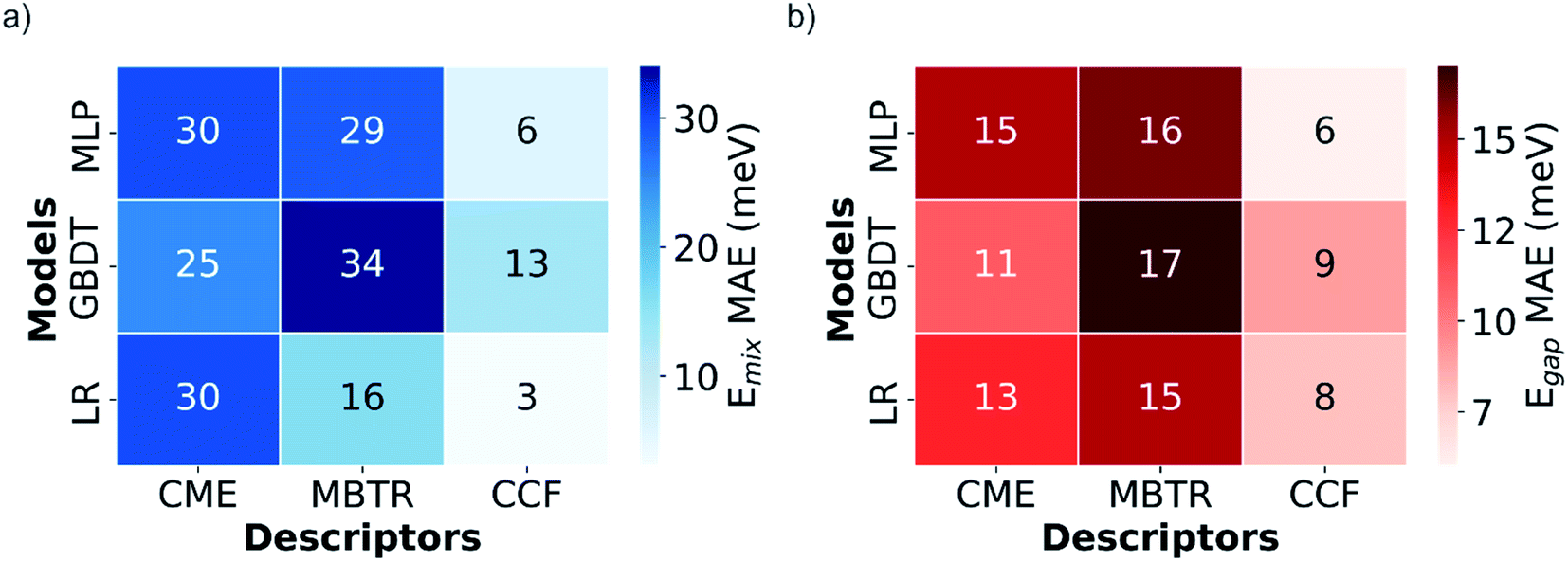Fig. 3 Heat maps with the mean absolute errors (MAE) of (a) mixing energy (E_mix) and (b) bandgap (E_g) predictions for the test set with different descriptors and models.

The CCFs descriptor outperforms the CME and MBTR, not only for mixing energies, which could be expected due to the additive character and linearity of this property, but also for bandgaps, where historically CCF-based methods have found more problems predicting the correct behavior.⁵³ Interestingly, this is the opposite of what was found in the previous study by Midgley et al.,³ where CME showed much better results than CCFs for the mixing energy and bandgap prediction in the configurational space of an (Mg,Zn)O solid solution. Further research including different alloys is needed to investigate how and why the best descriptor depends on the nature of the alloy system. For the moment, we suggest that the nature of the chemical bonding in the different systems might play an important role. The more local character of CCFs, which describes mainly short distance arrangements of atoms through clusters, might be more suitable for covalent systems like this spinel, whereas the CME better captures the long-range interactions in a more ionic system like the (Mg,Zn)O solid solution.

The LR model is the best for describing mixing energies, at least with the local descriptors, MBTR and CCFs, reflecting the fact that energies are additive with respect to local contributions. However, when predicting bandgaps with the CCFs descriptor, the non-linearity of the MLP neural network permits it to outperform the LR model. The small difference between models might justify the use of simpler linear models in some cases, when training time and resources could be a limitation or a concern. Beyond the difference in the descriptor, the results of the best performing methods are very similar to those obtained for (Mg,Zn)O in ref. 3, considering the spread of the values for each system, and are accurate enough to be used confidently, the best test MAEs being equal to 3 and 6 meV for mixing energies and bandgap values respectively.

Different models can show large variations in performance depending on training data size; we now look at this effect. For this analysis, we focus on CCFs as the best descriptor and reduce the size of the training set to 505 or 202 configurations (50% and 20% of the total number of DFT-calculated structures, instead of the 80% used previously). The results of these tests are displayed in Fig. 4, where the CCF descriptor is the input for all models. The percentages presented there are referenced to the total number of configurations in the configurational space, corresponding to 5%, 12% and 19%, approximately. From there it can be clearly seen that, even with those reduced percentages, MLP and LR perform almost with the same accuracy, although GBDT drastically drops in its predictions, especially for the smallest set. Trends in here suggest that using bigger training sets could improve MLP performance, even with MAE values below those showed by LR for mixing energies, but at an increased cost that might not be worth it considering the already good results obtained with LR.

Fig. 4 Mean absolute errors evolution upon train set size in the predictions of (a) mixing energies and (b) bandgaps with CCFs as descriptor and for the different models tested.

Fig. 5a and b present a direct comparison between calculated and predicted values of the test set, according to the best performing model–descriptor pair for each property. The high accuracy for mixing energies is clearly noticeable with a R² value close to unity. For bandgaps the metrics are also very good, with maximum errors below 30 meV.

Fig. 5 Correlation between ML-predicted and DFT-calculated values in the test set for (a) mixing energies and (b) bandgaps, including detailed metrics of performance. Also, ML-predicted (blue dots) and DFT-calculated (green crosses) values of (c) mixing energies and (d) bandgaps plotted against the inversion degree of the configuration.

Despite these positive results, it can be seen that errors in the prediction of bandgaps are mainly concentrated at the low ends of the inversion degree and band gap ranges, where the model is less accurate because of the lack of similar structures for training. That issue can be studied in more detail by plotting both calculated and predicted values against the inversion degree of the configurations, as shown in Fig. 5c and d. While for mixing energies there are no noticeable differences between calculations and predictions, for the case of bandgaps there are some poorer predictions. For example, the only configuration with inversion degree y = 0 is one of the worst predictions within the test set, with the bandgap being significantly overestimated. Also, the configuration with the lowest calculated bandgap, with inversion degree y = 0.5 is notably underestimated. In any case, those configurations are well identified and the errors are still small (at worst of a few tens of meV). Clearly, the CCF-based models are excellent for making predictions in the configurational space of this solid solution.

3.3 Feature importance analysis

The absolute values of the coefficients of the linear models provide a measure of the importance of every descriptor (cluster) for predictions. For non-linear models, more advanced tools based on game theory, implemented on the SHAP Python library, are used with the same purpose. Applied to CCFs, we can see which kinds of clusters are those with more influence on the different results of both properties. Fig. 6a presents the linear coefficients for the different clusters within the LR model for predicting mixing energies. The results of the SHAP analysis for both properties are also presented in Fig. 6b and c, where the LR model is used for the mixing energy and the MLP model is used for the band gaps. Within our CCFs definition, clusters 1 and 2 correspond to the single-site clusters for the different coordination sites (octahedral or tetrahedral), clusters from 3 to 9 correspond to site-pair clusters, while the rest represent clusters of three sites. It is also significant that, within groups of the same order, the clusters with the lower index represent groups of atoms of greater proximity than those with a higher index in the same group. In Fig. 6b and c, the k parameter stands for the order (k = 1, 2 or 3) and the l parameter (in Å) stands for the maximum distance between atoms of the cluster. Details for all clusters in the expansion are given in Table S4 of the ESI.†

Fig. 6 (a) Linear coefficients for every cluster (for orders k = 1, 2, and 3) in the LR model used to predict mixing energies. SHAP analysis of the impact of the different clusters within the CCFs on the predicted values of (b) mixing energy (LR model) and (c) bandgap (MLP model), where l (in Å) is the maximum distance between atoms of the cluster.

From the figures of the SHAP analysis and the linear coefficients presented in Fig. 6a and b, it can be seen that, when predicting mixing energies, the most important cluster is the single-site cluster for octahedral positions (cluster #1). Cluster #2 is the single-site cluster for tetrahedral positions, but because the total composition over the two sites is fixed, this cluster does not offer any additional degree of freedom and has formally zero importance. Subsequently, the next clusters in terms of relevance are clusters from 5 to 9, which are clusters of order two. Thus, mixing energies are mainly defined by the inversion degree and by pair clusters to a lesser extent. This conclusion is consistent with the local character of the configuration energies, which, as previously said, have been traditionally described using CCFs within the cluster expansion method.

On the other hand, Fig. 6c shows that the most important clusters when predicting bandgaps are mainly clusters of order three. For predicting bandgaps, the specific arrangement of Sn and Ge atoms within the octahedral and tetrahedral lattice is thus much more important than for predicting mixing energies. It is also interesting to note that the weight of importance is not skewed so strongly to just a few important features when considering bandgap predictions (as opposed to mixing energy predictions), suggesting that the contributions from features is more evenly distributed over the full set for predicting band gaps. The most important clusters involve mainly octahedral positions, although the effect of clusters involving tetrahedral positions is not negligible. This analysis is consistent with the bandgap being a global property of the ion distribution, rather than arising from the addition of local contributions (as in the case of the energy). Long-range interactions and atom arrangement patterns play a key role in determining the bandgap.

We can gain additional physical insight to the performance of CCFs by investigating the normalized covariance matrix from the values of the different clusters (Fig. 7), defined as follows:

where α and β represent two clusters, X_mα and X_mβ are individual components of the CCF corresponding to these clusters over each the M configurations, and μ and σ represent the mean and the standard deviation of the M values of the CCF component for the given cluster. This matrix shows that, apart from clusters 1 and 2, there is no strictly redundant information because of the existence of direct or inverse correlation between cluster values. The correlation values between clusters are in general higher (in absolute value, meaning strong direct or inverse correlations) for pair clusters, where strong correlation between clusters involving tetrahedral and octahedral sites is noticed. However, that effect is much weaker in trios, which could be the reason for the higher complexity of bandgap predictions.

Fig. 7 Covariance matrix of the different values within the CCFs.

3.4 Applications of the predicted results for the full configuration space

We now illustrate the usefulness of being able to evaluate properties in the full configurational space of the simulation cell (the conventional cubic unit cell), thanks to the ML model, which was trained with DFT data from just a small subset of that space. We will first discuss the identification of optimal configurations (e.g., the lowest-energy one, or the configuration with minimum or maximum bandgap), and then the calculation of equilibrium properties.

A configurational map for the two studied properties is presented in Fig. 8a, giving us a broad perspective of the complete configurational space in the simulation cell. This plot illustrates the mild inverse correlation between mixing energy and bandgap (R² = 0.405), which implies that there will be a thermodynamic preference for the widest bandgaps. The marked dependence of the mixing energy on the inversion degree is apparent from the plot, the bandgap has a less marked correlation with the inversion degree, but some structure in this relationship is still apparent. The map also allows us to identify the extremal configurations, i.e., those with the highest and lowest bandgaps and mixing energies. Those configurations have been highlighted in the map and their structures, along with their space symmetry group, are also presented in Fig. 8b.

Fig. 8 (a) Distribution of predicted mixing energies and bandgaps for all the inequivalent Ge/Sn configurations in the GeSn₂N₄ cubic unit cell. Different colors represent different inversion degrees. (b) Structures of extremal configurations: the P4₁22 configuration has the lowest energy, the C2/m configuration has the widest bandgap, and the R3m configuration has the narrowest bandgap but highest energy. Sn in blue, Ge in green.

The most energetically favorable configuration, which also exhibits one of the widest bandgaps (2.03 eV) within the configurational space, belongs to the P4₁22 space group. This configuration is fully inverted, i.e., it has tetrahedral sites fully occupied by Sn, whereas the octahedral sites contain both Sn and Ge atoms in an ordered pattern. This ordered configuration corresponds to the tetragonal structure of Zn₂TiO₄,⁵⁴ and is known to be the configurational groundstate for other inverse spinels.^55–58 It has two distinct octahedral sites, on which the two cations are ordered. Although the P4₁22 configuration has a very wide bandgap, the widest bandgap (2.04 eV) configuration is another fully inverted one with C2/m symmetry and a mixing energy not much higher than the P4₁22 configuration. The least stable configuration, with the highest mixing energy and the lowest bandgap (1.31 eV), is a structure with an inversion degree y = 0.5 and R3m space group and has a quasi-2D structure with alternating layers of Sn and Ge cations. Interestingly, the next least stable structure (top right corner of Fig. 8a) is the ideal spinel structure with inversion degree y = 0, which has one of the highest bandgaps.

The analysis above refers to the properties of individual configurations. However, given the small energy differences in the configurational space, we can expect that there will be a large degree of disorder in the GeSn₂N₄ structure, which we will discuss now based on the full configurational energy spectrum. For the determination of the equilibrium degree of inversion from first-principles calculations, it is common to adopt a simple 3-point model^30,59–61 based on the DFT energies of the primitive cell in its three possible degrees of inversion, y = 0, 0.5, and 1 (there is only one symmetrically different configuration of cations for each value of y in this cell). In this model the inversion energy, E_inv(y), is a quadratic fit of the DFT energies, and the equilibrium degree of inversion at a given temperature T is given by the minimum of the inversion free energy:

F_inv(y,T) = E_inv(y) − TS_inv(y)

where
is the “ideal” configurational entropy of inversion, assuming no energy differences between configurations with the same degree of inversion (k_B is Boltzmann's constant). For our system, this model leads to the prediction of an almost fully inverted supercell at any temperature of interest, as shown in Fig. 9. The advantage of this model is that it does not require the evaluation of DFT energies in a large configurational space, but only three energies in a small supercell. However, the underlying assumption that the energy is only a function of inversion degree is not correct for GeSn₂N₄, as has been demonstrated above. Having access to all the energies (and other properties) in the much larger configurational space for the cubic conventional cell allows us to perform more accurate configurational statistics. The equilibrium degree of inversion, for example, can be calculated as:
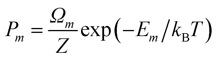
where
is the Boltzmann probability of configuration m, with degeneracy Ω_m and an energy E_m as predicted from the ML model, M = 4222 is the total number of symmetrically distinct configurations in the cubic unit cell, and Z is the partition function that guarantees that the sum of probabilities is one.^43,62 In contrast with the result from the 3-point model, the equilibrium degree of inversion calculated via configurational averaging departs significantly from 1. In principle, for even more accurate configurational statistics, we would need to do this analysis in increasingly larger supercells to check for convergence, using a Monte Carlo method for sampling instead of systematic enumeration. This would be possible for the calculation of energies via cluster expansions, which can be transferred to larger supercell (although similar extrapolations to larger cells are not trivial for the non-linear, or even linear, band gap models). In fact, in the configurational space of the cubic unit cell, using only the 1013 points directly calculated from DFT leads to equilibrium inversion degrees that differ by less than 4% from those calculated with all the 4222 distinct configurations. To take full advantage of the ML models one would need to work in larger supercells, or decrease the number of DFT points used for training. Here, we will not further discuss cell size effects, but the transferability to larger cells of site-occupancy models, beyond the case of a simple cluster expansion, deserves investigation in future work.

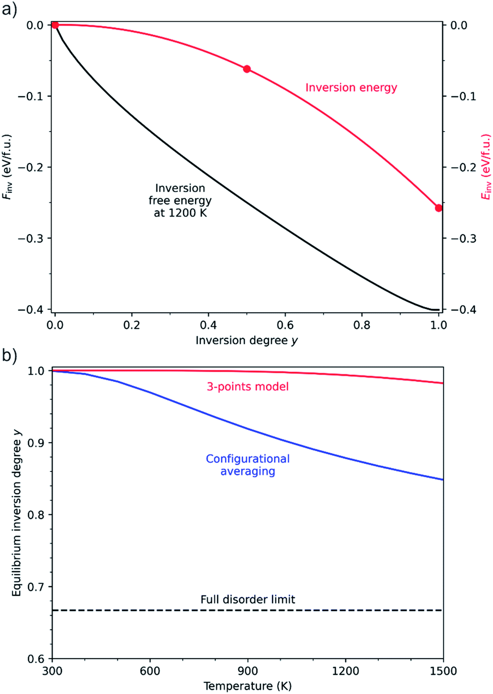Fig. 9 (a) Inversion energy (in red) calculated with the 3-point model, and the corresponding free energy at 1200 K. (b) Equilibrium degree of inversion predicted from averaging in the 4222-point configurational space (in blue), in comparison with the prediction from the 3-point model (in red) and the full-disorder limit (black dashed line).

The actual cation distribution in the GeSn₂N₄ system will depend on the thermal history of the sample; in particular the rate of cooling after synthesis is a parameter that is sometimes used to control the ionic distribution.^63,64 If the system is allowed to equilibrate at low temperatures (say if annealed very slowly), the inversion will be almost complete (y ≈ 1). But if the synthesis procedure somehow freezes the high temperature disorder, say by rapid quenching after synthesis, an incomplete inversion might be achieved. Control of the cation distribution in this way is interesting and might have practical applications, because it provides a route to tune the bandgap, and perhaps other properties, of the system. In the low temperature limit, the bandgap equals the gap of the lowest-energy configuration, 2.03 eV, whereas in the high-temperature limit, with a random cation distribution corresponding to y = 2/3 (i.e., equal to the Sn/(Sn + Ge) ratio), the average bandgap reduces to 1.87 eV. These useful predictions require knowledge of energies and bandgaps in a large space of (at least) thousands of cation distribution configurations, so this type of analysis in other systems would be very computationally expensive if it was not accelerated by the ML techniques presented in this work.

4. Conclusions

We have presented an accurate and interpretable description of the whole configurational space of γ-phase GeSn₂N₄ nitrides, at a greatly reduced cost, through the combined use of DFT calculations and ML techniques. Our ML models, trained on DFT results from a small fraction (20% at most) of the structures within the space, exhibit excellent performance metrics, with mean errors in the range of few meV and almost perfect correlation between ML-predicted and DFT-calculated values.

Our results provide useful methodological information to perform this type of study in the future. We have compared the performance of different descriptors and models and found the optimal combinations for each task. In this case, a linear model based on cluster correlation functions, i.e., a cluster expansion, is shown to be the best model for the energies. For bandgap predictions in the configurational space, the non-linearity of the neural network (based on cluster correlation functions) has the best performance. Explainable ML highlights difference between energy and bandgap predictions, for the latter, the most relevant clusters are not necessarily the smallest and lowest-order ones, which means that cluster expansions of the bandgap, even non-linear ones, require a cluster basis of at least order three and may improve with higher order basis. It is interesting, from the comparison with previous work, that the conclusions about the best descriptors and models are not universal. It is unclear so far how the optimal model depends on the nature of the solid solution, and this will be the subject of future research.

For the spinel nitrides considered here, we have seen that the configuration energies are mainly, though not completely, influenced by the inversion degree, and to a lesser extent by pair-type clusters. High inversion degrees, i.e., Sn occupation of tetrahedral positions, are clearly favored. However, we have demonstrated that the accurate calculation of the equilibrium inversion degree at a given temperature requires consideration of the energy differences at a given degree of inversion, thus illustrating the limitations of traditional equilibrium inversion models for spinels. Our combined DFT and ML model allows us to predict that the bandgap of this solid solution can be potentially tuned via modifications of the cation distribution in the system. The combination of methods that we have demonstrated and the insights that we have obtained should be applicable to many other alloy and solid solution systems.

Data availability

The code and data to reproduce the results in this paper are available at https://github.com/pablos-pv/GeSn2N4_ML. Complete sets of raw data and an archived version of the code are available at: https://zenodo.org/record/6974760

Conflicts of interest

The authors declare that they have no known competing financial interests or personal relationships that could have appeared to influence the work reported in this paper.

Acknowledgements

This work was accomplished thanks to the mobility grants given by Universidad Politécnica de Madrid Programa Propio de I + D + I 2021 and ERASMUS++ European project. P. S.-P. and P. P. acknowledge support from Ministerio de Ciencia e Innovación through the project BESTMAT-QC (PID2019-107137RB-C22). S. H. also acknowledges funding from the Agencia Estatal de Investigación and the Ministerio de Ciencia, Innovación y Universidades, of Spain (PID2019-110430 G B-C22), and from the EU FEDER Framework 2014-2020 and Consejería de Conocimiento, Investigación y Universidad of the Andalusian Government (FEDER-UPO-1265695). The authors also gratefully acknowledge the UK Materials and Molecular Modelling Hub, which is partially funded by EPSRC (EP/T022213/1), for providing computing resources on the Young supercomputer.

References

1. P. Hohenberg and W. Kohn, Inhomogeneous Electron Gas, Phys. Rev., 1964, 136(3B), 864–871,  DOI:10.1103/PhysRev.136.B864.
2. W. Kohn and L. J. Sham, Self-Consistent Equations Including Exchange and Correlation Effects, Phys. Rev., 1965, 140(4A), 1133–1138,  DOI:10.1103/PhysRev.140.A1133.
3. S. D. Midgley, S. Hamad, K. T. Butler and R. Grau-Crespo, Bandgap Engineering in the Configurational Space of Solid Solutions via Machine Learning: (Mg,Zn)O Case Study, J. Phys. Chem. Lett., 2021, 12(21), 5163–5168,  DOI:10.1021/acs.jpclett.1c01031.
4. G. L. W. Hart, T. Mueller, C. Toher and S. Curtarolo, Machine learning for alloys, Nat. Rev. Mater., 2021, 6(8), 730–755,  DOI:10.1038/s41578-021-00340-w.
5. M. Yaghoobi and M. Alaei, Machine learning for compositional disorder: a comparison between different descriptors and machine learning frameworks, Comput. Mater. Sci., 2022, 207, 111284,  DOI:10.1016/j.commatsci.2022.111284.
6. E. M. Askanazi, S. Yadav and I. Grinberg, Prediction of the Curie temperatures of ferroelectric solid solutions using machine learning methods, Comput. Mater. Sci., 2021, 199, 110730,  DOI:10.1016/j.commatsci.2021.110730.
7. P. Pentyala, V. Singhania, V. K. Duggineni and P. A. Deshpande, Machine learning-assisted DFT reveals key descriptors governing the vacancy formation energy in Pd-substituted multicomponent ceria, Mol. Catal., 2022, 522, 112190,  DOI:10.1016/j.mcat.2022.112190.
8. Z. Pei, J. Yin, J. A. Hawk, D. E. Alman and M. C. Gao, Machine-learning informed prediction of high-entropy solid solution formation: beyond the Hume-Rothery rules, npj Comput. Mater., 2020, 6, 50,  DOI:10.1038/s41524-020-0308-7.
9. M. Chandran, S. C. Lee and S. J. hyeok, Machine learning assisted first-principles calculation of multicomponent solid solutions: estimation of interface energy in Ni-based superalloys, Model. Simul. Mater. Sci. Eng., 2018, 26, 025010,  DOI:10.1088/1361-651X/aa9f37.
10. K. Morita, D. W. Davies, K. T. Butler and A. Walsh, Modeling the dielectric constants of crystals using machine learning, J. Chem. Phys., 2020, 153, 024503,  DOI:10.1063/5.0013136.
11. K. T. Butler, M. D. Le, J. Thiyagalingam and T. G. Perring, Interpretable, calibrated neural networks for analysis and understanding of inelastic neutron scattering data, J. Phys. Condens. Matter, 2021, 33, 194006,  DOI:10.1088/1361-648X/abea1c.
12. S. D. Mo, L. Ouyang, W. Y. Ching, I. Tanaka, Y. Koyama and R. Riedel, Interesting physical properties of the new spinel phase of Si₃N₄ and C₃N₄, Phys. Rev. Lett., 1999, 83(24), 5046–5049,  DOI:10.1103/PhysRevLett.83.5046.
13. A. Zerr, G. Miehe and G. Serghiou, et al., Synthesis of cubic silicon nitride, Nature, 1999, 400, 340–342,  DOI:10.1038/22493.
14. A. Zerr, R. Riedel, T. Sekine, J. E. Lowther, W. Y. Ching and I. Tanaka, Recent advances in new hard high-pressure nitrides, Adv. Mater., 2006, 18(22), 2933–2948,  DOI:10.1002/adma.200501872.
15. T. D. Boyko and A. Moewes, The hardness of group 14 spinel nitrides revisited, J. Ceram. Soc. Japan, 2016, 124(10), 1063–1066,  DOI:10.2109/jcersj2.16097.
16. H. Hu and G. H. Peslherbe, Accurate Mechanical and Electronic Properties of Spinel Nitrides from Density Functional Theory, J. Phys. Chem. C, 2021, 125(17), 8927–8937,  DOI:10.1021/acs.jpcc.0c09896.
17. T. D. Boyko, A. Hunt, A. Zerr and A. Moewes, Electronic structure of spinel-type nitride compounds Si₃N₄, Ge₃N₄, and Sn₃N₄ with tunable band gaps: Application to light emitting diodes, Phys. Rev. Lett., 2013, 111(9), 097402,  DOI:10.1103/PhysRevLett.111.097402.
18. C. M. Caskey, J. A. Seabold and V. Stevanović, et al., Semiconducting properties of spinel tin nitride and other IV₃N₄ polymorphs, J. Mater. Chem. C, 2015, 3(6), 1389–1396,  10.1039/c4tc02528h.
19. F. Qu, Y. Yuan and M. Yang, Programmed Synthesis of Sn₃N₄ Nanoparticles via a Soft Chemistry Approach with Urea: Application for Ethanol Vapor Sensing, Chem. Mater., 2017, 29(3), 969–974,  DOI:10.1021/acs.chemmater.6b03435.
20. X. Li, A. L. Hector, J. R. Owen and S. I. U. Shah, Evaluation of nanocrystalline Sn₃N₄ derived from ammonolysis of Sn(NEt₂)₄ as a negative electrode material for Li-ion and Na-ion batteries, J. Mater. Chem. A, 2016, 4(14), 5081–5087,  10.1039/c5ta08287k.
21. J. Wang, H. Chen, S. H. Wei and W. J. Yin, Materials Design of Solar Cell Absorbers Beyond Perovskites and Conventional Semiconductors via Combining Tetrahedral and Octahedral Coordination, Adv. Mater., 2019, 31(17), 1806593,  DOI:10.1002/adma.201806593.
22. C. W. Rosenbrock, K. Gubaev and A. V. Shapeev, et al., Machine-learned interatomic potentials for alloys and alloy phase diagrams, npj Comput. Mater., 2021, 7, 24,  DOI:10.1038/s41524-020-00477-2.
23. T. Kostiuchenko, F. Körmann, J. Neugebauer and A. Shapeev, Impact of lattice relaxations on phase transitions in a high-entropy alloy studied by machine-learning potentials, npj Comput. Mater., 2019, 5, 55,  DOI:10.1038/s41524-019-0195-y.
24. T. A. A. Batchelor, J. K. Pedersen, S. H. Winther, I. E. Castelli, K. W. Jacobsen and J. Rossmeisl, High-Entropy Alloys as a Discovery Platform for Electrocatalysis, Joule, 2019, 3(3), 834–845,  DOI:10.1016/j.joule.2018.12.015.
25. S. Sun, A. Tiihonen and F. Oviedo, et al., A data fusion approach to optimize compositional stability of halide perovskites, Matter, 2021, 4(4), 1305–1322,  DOI:10.1016/j.matt.2021.01.008.
26. A. G. Kusne, H. Yu and C. Wu, et al., On-the-fly closed-loop materials discovery via Bayesian active learning, Nat. Commun., 2020, 11(1), 1–11,  DOI:10.1038/s41467-020-19597-w.
27. P. Sánchez-Palencia, G. García, J. C. Conesa, P. Wahnón and P. Palacios, Spinel-Type nitride compounds with improved features as solar cell absorbers, Acta Mater., 2020, 197, 316–329,  DOI:10.1016/j.actamat.2020.07.034.
28. J. N. Hart, N. L. Allan and F. Claeyssens, Ternary silicon germanium nitrides: A class of tunable band gap materials, Phys. Rev. B: Condens. Matter Mater. Phys., 2011, 84(24) DOI:10.1103/PhysRevB.84.245209.
29. S. V. Dudiy and A. Zunger, Searching for alloy configurations with target physical properties: impurity design via a genetic algorithm inverse band structure approach, Phys. Rev. Lett., 2006, 97(4), 1–4,  DOI:10.1103/PhysRevLett.97.046401.
30. Y. Seminovski, P. Palacios, P. Wahnón and R. Grau-Crespo, Band gap control via tuning of inversion degree in CdIn₂S₄ spinel, Appl. Phys. Lett., 2012, 100, 102112,  DOI:10.1063/1.3692780.
31. S. Roychowdhury, T. Ghosh and R. Arora, et al., Enhanced atomic ordering leads to high thermoelectric performance in AgSbTe₂, Science, 80-2021, 371(6530), 722–727,  DOI:10.1126/science.abb3517.
32. R. Nechache, C. Harnagea and S. Li, et al., Bandgap tuning of multiferroic oxide solar cells, Nat. Photonics, 2014, 9, 61–67,  DOI:10.1038/nphoton.2014.255.
33. Y. Wang, S. R. Kavanagh, I. Burgués-Ceballos, A. Walsh, D. O. Scanlon and G. Konstantatos, Cation disorder engineering yields AgBiS₂ nanocrystals with enhanced optical absorption for efficient ultrathin solar cells, Nat. Photonics, 2022, 16, 235–241,  DOI:10.1038/s41566-021-00950-4.
34. S. M. Lundberg and S. I. Lee, A Unified Approach to Interpreting Model Predictions, in NIPS'17: Proceedings of the 31st International Conference on Neural Information Processing Systems, ed. U. von Luxburg, I. Guyon, S. Bengio, H. Wallach and R. Fergus, Curran Associates Inc., 2017, pp. 4768–4777.
35. G. Kresse and J. Furthmüller, Efficiency of ab-initio total energy calculations for metals and semiconductors using a plane-wave basis set, Comput. Mater. Sci., 1996, 6(1), 15–50,  DOI:10.1016/0927-0256(96)00008-0.
36. G. Kresse and J. Furthmüller, Efficient iterative schemes for ab initio total-energy calculations using a plane-wave basis set, Phys. Rev. B: Condens. Matter Mater. Phys., 1996, 54(16), 169–186,  DOI:10.1103/PhysRevB.54.11169.
37. P. E. Blöchl, Projector augmented-wave method, Phys. Rev. B: Condens. Matter Mater. Phys., 1994, 50(24), 17953–17979,  DOI:10.1103/PhysRevB.50.17953.
38. J. P. Perdew, K. Burke and M. Ernzerhof, Generalized gradient approximation made simple, Phys. Rev. Lett., 1996, 77(18), 3865–3868,  DOI:10.1103/PhysRevLett.77.3865.
39. J. Hubbard, Electron correlations in narrow energy bands, Proc. R. Soc. London, Ser. A, 1963, 276(1365), 238–257,  DOI:10.1098/rspa.1963.0204.
40. S. Dudarev and G. Botton, Electron-energy-loss spectra and the structural stability of nickel oxide: An LSDA+U study, Phys. Rev. B: Condens. Matter Mater. Phys., 1998, 57(3), 1505–1509,  DOI:10.1103/PhysRevB.57.1505.
41. J. Heyd, G. E. Scuseria and M. Ernzerhof, Hybrid functionals based on a screened Coulomb potential, J. Chem. Phys., 2003, 118(18), 8207–8215,  DOI:10.1063/1.1564060.
42. E. Feldbach, A. Zerr and L. Museur, et al., Electronic Band Transitions in γ-Ge₃N₄, Electron. Mater. Lett., 2021, 17(4), 315–323,  DOI:10.1007/s13391-021-00291-y.
43. R. Grau-Crespo, S. Hamad, C. R. A. Catlow and N. H. De Leeuw, Symmetry-adapted configurational modelling of fractional site occupancy in solids, J. Phys. Condens. Matter, 2007, 19(25), 256201,  DOI:10.1088/0953-8984/19/25/256201.
44. J. Schmidt, M. R. G. Marques, S. Botti and M. A. L. Marques, Recent advances and applications of machine learning in solid-state materials science, npj Comput. Mater., 2019, 5, 83,  DOI:10.1038/s41524-019-0221-0.
45. F. Faber, A. Lindmaa, O. A. Von Lilienfeld and R. Armiento, Crystal structure representations for machine learning models of formation energies, Int. J. Quantum Chem., 2015, 115(16), 1094–1101,  DOI:10.1002/qua.24917.
46. M. Rupp, A. Tkatchenko, K. R. Müller and O. A. Von Lilienfeld, Fast and accurate modeling of molecular atomization energies with machine learning, Phys. Rev. Lett., 2012, 108, 058301,  DOI:10.1103/PhysRevLett.108.058301.
47. H. Huo and M. Rupp, Unified Representation of Molecules and Crystals for Machine Learning, Published online, 2017, 10.48550/arXiv.1704.06439.
48. J. M. Sanchez, F. Ducastelle and D. Gratias, Generalized cluster description of multicomponent systems, Phys. A, 1984, 128(1–2), 334–350,  DOI:10.1016/0378-4371(84)90096-7.
49. M. Troppenz, S. Rigamonti and C. Draxl, Predicting Ground-State Configurations and Electronic Properties of the Thermoelectric Clathrates Ba₈Al_xSi_46-x and Sr₈Al_xSi_46-x, Chem. Mater., 2017, 29(6), 2414–2424,  DOI:10.1021/acs.chemmater.6b05027.
50. R. Tibshirani, Regression Shrinkage and Selection Via the Lasso, J. R. Stat. Soc., 1996, 58(1), 267–288,  DOI:10.1111/j.2517-6161.1996.tb02080.x.
51. J. H. Friedman, Stochastic gradient boosting, Comput. Stat. Data Anal., 2002, 38(4), 367–378,  DOI:10.1016/S0167-9473(01)00065-2.
52. K. Hornik, M. Stinchcombe and H. White, Multilayer feedforward networks are universal approximators, Neural Network., 1989, 2(5), 359–366,  DOI:10.1016/0893-6080(89)90020-8.
53. X. Xu and H. Jiang, Cluster expansion based configurational averaging approach to bandgaps of semiconductor alloys, J. Chem. Phys., 2019, 150(3), 034102,  DOI:10.1063/1.5078399.
54. J. Liu, X. Wang and O. J. Borkiewicz, et al., Unified View of the Local Cation-Ordered State in Inverse Spinel Oxides, Inorg. Chem., 2019, 58(21), 14389–14402,  DOI:10.1021/acs.inorgchem.9b01685.
55. V. Stevanović, M. D'Avezac and A. Zunger, Simple point-ion electrostatic model explains the cation distribution in spinel oxides, Phys. Rev. Lett., 2010, 105(7), 11–14,  DOI:10.1103/PhysRevLett.105.075501.
56. A. Seko, F. Oba and I. Tanaka, Classification of spinel structures based on first-principles cluster expansion analysis, Phys. Rev. B: Condens. Matter Mater. Phys., 2010, 81, 054114,  DOI:10.1103/PhysRevB.81.054114.
57. A. Seko, K. Yuge, F. Oba, A. Kuwabara and I. Tanaka, Prediction of ground-state structures and order-disorder phase transitions in II-III spinel oxides: a combined cluster-expansion method and first-principles study, Phys. Rev. B: Condens. Matter Mater. Phys., 2006, 73, 184117,  DOI:10.1103/PhysRevB.73.184117.
58. B. A. Wechsler and A. Navrotsky, Thermodynamics and structural chemistry of compounds in the system MgO□TiO₂, J. Solid State Chem., 1984, 55(2), 165–180,  DOI:10.1016/0022-4596(84)90262-7.
59. D. Santos-Carballal, A. Roldan, R. Grau-Crespo and N. H. De Leeuw, First-principles study of the inversion thermodynamics and electronic structure of FeM2X4 (thio)spinels (M=Cr, Mn, Co, Ni; X= O, S), Phys. Rev. B: Condens. Matter Mater. Phys., 2015, 91, 195106,  DOI:10.1103/PhysRevB.91.195106.
60. H. S. C. O'Neill and A. Navrotsky, Simple spinels: crystallographic parameters, cation radii, lattice energies, and cation distribution, Am. Mineral., 1983, 68, 181–194.
61. H. B. Callen, S. E. Harrison and C. J. Kriessman, Cation distributions in ferrospinels. Theoretical, Phys. Rev., 1956, 103(4), 851–856,  DOI:10.1103/PhysRev.103.851.
62. R. Grau-Crespo and U. V. Waghmare, Simulation of Crystals with Chemical Disorder at Lattice Sites, in Molecular Modeling for the Design of Novel Performance Chemicals and Materials, ed. B. Rai, CRC Press, 2012, pp. 319–342, DOI:  DOI:10.1201/b11590-12.
63. A. Gautam, M. Sadowski and N. Prinz, et al., Rapid Crystallization and Kinetic Freezing of Site-Disorder in the Lithium Superionic Argyrodite Li₆PS₅Br, Chem. Mater., 2019, 31(24), 10178–10185,  DOI:10.1021/acs.chemmater.9b03852.
64. S. A. Redfern, R. J. Harrison, H. S. C. O’Neill and D. R. Wood, Thermodynamics and kinetics of cation ordering in MgAl₂O₄ spinel up to 1600 C from in situ neutron diffraction, Am. Mineral., 1999, 84, 299–310,  DOI:10.2138/am-1999-0313.
65. F. Oviedo, J. L. Ferres, T. Buonassisi and K. T. Butler, Interpretable and explainable machine learning for materials science and chemistry, Acc. Mater. Res., 2022, 3, 597–607,  DOI:10.1021/accountsmr.1c00244.

---

Footnote

† Electronic supplementary information (ESI) available. See https://doi.org/10.1039/d2dd00038e

---