A Δ-machine learning approach for force fields, illustrated by a CCSD(T) 4-body correction to the MB-pol water potential

Abstract

Δ-Machine learning (Δ-ML) has been shown to effectively and efficiently bring a low-level ML potential energy surface to CCSD(T) quality. Here we propose extending this approach to general force fields, which implicitly or explicitly contain many-body effects. After describing this general approach, we illustrate it for the MB-pol water potential which contains CCSD(T) 2-body and 3-body interactions but relies on the TTM4-F 4-body and higher body interactions. The 4-body MB-pol (TTM4-F) interaction fails at very short range and for the water hexamer errors up to 0.84 kcal mol⁻¹ are seen for some isomers, owing mainly to 4-body errors. We apply Δ-ML for the 4-body interaction, using a recent dataset of CCSD(T) 4-body energies that we used to develop a new water potential, q-AQUA. This 4-body correction is shown to improve the accuracy of the MB-pol potential for the relative energies of 8 isomers of the water hexamer as well as the harmonic frequencies. The new potential is robust in the very short range and so should be reliable for simulations at high pressure and/or high temperature.

---

Introduction

Machine learning (ML) correction methods aim to elevate the level of accuracy of ML properties, for example potential energy surfaces (PESs). There are two approaches currently being investigated to accomplish this goal. One is transfer learning, which has been developed extensively in the context of artificial neural networks,¹ and much of the work in that field has been brought into chemistry, especially in the development of PESs.^2–4 For example, Meuwly and co-workers applied transfer learning using thousands of local CCSD(T) energies to improve their MP2-based neural network PESs for malonaldehyde, acetoacetaldehyde and acetylacetone.³ The basic idea of transfer learning is that a fit obtained from one source of data (perhaps a large one) can be fine-tuned for a related problem by using limited data. Therefore, in the present context of PES fitting, an ML-PES trained with low-level electronic energies/gradients can be reused as the starting point of the model for an ML-PES with the accuracy of a high-level electronic structure theory. As noted, this is typically done with artificial neural networks, where weights and biases trained on lower-level data hopefully require minor changes in response to additional training using high-level data.

The other approach is Δ-machine learning. In this approach a correction is made to a property obtained using an efficient, low-level ab initio theory.^5–8 We recently proposed and tested a Δ-ML approach, that uses a small number of CCSD(T) energies, to correct a low-level PES based on DFT electronic energies and gradients.^9,10 The equation for this approach is simply

V_LL→CC = V_LL + ΔV_CC–LL, (1)

where V_LL→CC is the corrected PES, V_LL is a PES fit to low-level electronic data (such as DFT energies and gradients), and ΔV_CC–LL is the correction based on high-level coupled cluster energies. It is noted that the difference between CCSD(T) and DFT energies, ΔV_CC–LL, is usually not as strongly varying as V_LL with respect to the nuclear configurations and therefore just a small number of high-level electronic energies are adequate to fit the correction PES. The method was validated for PESs of small molecules, CH₄ and H₃O⁺, 12-atom N-methyl acetamide, and 15-atom acetylacetone. In all cases, the coupled cluster energies were obtained over the same large span of configurations used to get the lower-level PES.

Here we propose to extend this Δ-ML approach from molecular PESs to general, non-reactive force fields that are explicitly or implicitly many-body. There are many examples of such force fields that determine the total energy of N monomers. For example, consider force fields for water. (For a recent review see ref. 11.) For simplicity, we denote these by “MB-FF”. Suppose our goal is to bring this force field to the “gold-standard” CCSD(T) level of theory. Clearly this cannot be done by simply applying the above equation for an arbitrary number of monomers owing to the prohibitively exponential computational cost of CCSD(T) calculations with respect to the number of monomers. Instead we propose a Δ-ML force-field for N monomers given by the sum of many-body corrections, namely

where ΔV_n-b are the many-body corrections to the MB-FF many-body terms, given by the difference between CCSD(T) and MB-FF n-body (n-b) interaction energies. To be clear, recall that the n-b interaction energy is obtained from a cluster of n monomers. For example, the 4-b interaction is obtained by calculating the total energy of the tetramer (four monomers) and subtracting all the 1-, 2-, and 3-b interactions from the total energy. Note for simplicity, we assume that an accurate 1-b term, e.g., the single water molecule, is given in the MB-FF.

We have truncated explicit correction terms at the 4-b level with force-fields for water in mind. This is because it has been established by high-level calculations that 4-b, while small, are needed to obtain nearly 100 percent of the electronic dissociation energies of water clusters up to the 21-mer.¹² This has also been shown previously for some isomers of the water hexamer^13,14 and we show this again explicitly here. And crucially, we have the CCSD(T) electronic energies needed for the correction up to 4-b, and these datasets were recently used to develop the pure many-body water potential q-AQUA.^15,16

where the meaning of each term is clear. In q-AQUA the 2-, 3-, and 4-b interactions are permutationally invariant polynomial (PIP)^17,18 fits to thousands of CCSD(T) energies (details are in ref. 16.) These CCSD(T) electronic energies for the 2-b, 3-b and 4-b are ready to be used to obtain a ΔV_n-b correction to any water MB-FF, and we return to this below.

In this work, the focus is on the 4-b correction to the MB-pol force field.^19,20 In MB-pol the 2-b and 3-b are already at CCSD(T) level, but the 4-b interaction is essentially given by the TTM4-F potential,²¹ which is a sophisticated MB-FF for water. Errors between 0.1 and 0.84 kcal mol⁻¹ for the these 4-b interactions for the hexamer isomers against direct CCSD(T) calculations, were reported in 2015.²² These are fairly large fractions of the 4-b energy itself. Stimulated by recent assessments of the importance of the 4-b interaction and inaccuracy of the MB-pol 4-b, we report a correction 4-b PES, denoted ΔV_4-b, that is aimed directly at extending the MB-pol potential to the CCSD(T) 4-b level. The correction is a PIP fit to the energy difference between the CCSD(T) 4-b interactions and TTM4-F 4-b interactions.

In the next section we present the details of the 4-b correction PES, followed by several tests that indicate the effectiveness of this correction PES.

ΔV_4-b fitting details

The data set for the ΔV_4-b fit is simply the difference between the 4-b CCSD(T)-F12/haTZ (aug-cc-pVTZ basis for O atoms and cc-pVTZ for H atoms) and MB-pol/TTM4-F energies. The total number of configurations in the data set is 3692 and all of them are used for the fit. The fit uses the PIP approach, in which the PIPs are generated using MSA software.^18,23 The PIPs are usually polynomials in the Morse variables of the internuclear distances, exp(−r_ij/λ), where r_ij is the distance between atoms i and j and λ is a range parameter, taken for this calculation to be 1.5 bohr. We used 22221111 permutational symmetry at a maximum polynomial order of 3. Two additional issues concerning the basis set are important to note.

First, it is desirable not to include polynomials that do not have the correct limiting behavior as one or more monomers are removed from the others to a large distance. In the 4-body case, we need to consider the removal of each monomer from the other three and the removal of each possible dimer from the other one. In all of these cases, the 4-body interaction energy must vanish. The process of identifying PIPs that do not have the correct limiting behavior is what we call purification.^24,25 To identify the PIPs with incorrect limiting behavior, the relevant distances are augmented by 100 Å, and we accept the polynomial as having the correct behavior if its Morse value is below 10⁻⁶. We cannot, however, immediately eliminate these polynomials because there may be other polynomials that, for example, are composed of products between one with a correct limit and one with an incorrect limit. At first, we simply rename the ones with an incorrect limit. After all the polynomials have been evaluated, we examine the definitions of all those with the correct limits and determine which of the monomials and which of the renamed polynomials with incorrect limits are required to calculate them. Finally, we remove those polynomials that are not required and renumber those that remain, keeping the order of calculation to ensure that no partial calculation that contributes to any polynomial needs to be performed twice. We then have a set of polynomials that all have the correct limiting behavior and that can be calculated efficiently.²⁶

The second issue that we need to consider is how to maintain permutational symmetry, not only in each monomer, but when monomers as a whole are interchanged with one another. This latter exchange is not taken into account by the MSA software, so the polynomials that we create by the previously described purification will not, in general, have permutational symmetry with respect to exchange of identical monomers. A common method for dealing with this issue is to augment the dataset by adding all relevant permutations of the Cartesian coordinates and assigning them the same energy, thus requiring a set of n! geometries for each energy, where n is the number of monomers (4, in this case). A better method is to identify groups of polynomials that have permutational symmetry with respect to monomer exchange and then form “superpolynomials” that are the sum of the polynomial members of each group. We identify the permutationally invariant groups of polynomials by taking a single set of n! permutationally related geometries and calculating the value of each polynomial. While the values of individual polynomials vary from permutation to permutation, the groups of polynomials, taken together for each permutation, will have the same group of values. For each permutation, one can form pairs of the polynomial identities and their values, and then sort the pairs by their values. Looking at all pairs that have the same value component in all permutations gives the identities of the polynomials, some of which may be repeated, that make up a permutationally invariant group. In general, there will be as many groups as there were original polynomials. These groups, each with n! (not necessarily unique) polynomial contributions, are then summed to form “superpolynomials” having permutational symmetry with respect to exchange of identical molecules. Having formed these superpolynomials, there is no need for augmentation of the dataset with permutationally related geometries.

We used basis sets of different sizes, with 200, 500, and 1000 “superpolynomials”. More details of the bases are given in Table 1. As seen, although fitting with more polynomials can reduce the fitting error, the computational cost is roughly proportional to the sum of the number of monomials and polynomials. The results presented in this paper are based on the basis with 200 “superpolynomials”, as this achieves reasonably good accuracy with smaller cost.

Table 1 Number of monomials (m), polynomials (q), and “super-polynomials” (p) in the three fitting bases used for ΔV_4-b, and corresponding fitting root-mean-square error (RMSE, in cm⁻¹) and computational time (in seconds) for 100 000 energy evaluations. The computational time for all gradients is about 3 times that for the energy²⁷

	PIP200	PIP500	PIP1000
Number of m	1438	3442	8610
Number of q	5490	12 898	25 084
Number of p	200	500	1000
Fitting RMSE	6.7	4.0	2.5
Timing	1.1	2.7	6.0

---

The final energy is written as

where S_ijkl is a switching function whose value is 1 at short range and 0 at the long range. Specifically,where r_max is the maximum OO distance in a water tetramer, and S is 1 when r_max is smaller than r_i and is 0 when r_max is greater than r_f. In this work we used r_i = 5.5 Å and r_f = 7.0 Å unless otherwise specified.

Results and discussions

First we examine two 1-d cuts where we compare the 4-b CCSD(T)-F12/haTZ energies to those from MB-pol/TTM4-F and to those from MB-pol + ΔV_4-b. Fig. 1 and 2 show cuts of the potential for separating two dimers from one another and for separating a monomer from the remaining trimer, respectively. The major improvements of the 4-b correction are in the short-range. Whereas MB-pol/TTM4-F is quite accurate in the long range, it is not designed with the proper Pauli exchange and repulsion in the short range. Despite the fact that TTM4-F fails badly in the short range, the Δ_4-b potential does provide a reasonable correction. It should be noted that for both cuts shown, the equilibrium R_OO distance is 2.7 Å, so that large corrections are in the steeply repulsive part of the potential. However, there are also large corrections for highly distorted tetramers geometries not visited by this cut, discussed below.

Fig. 1 4-b energies from indicated sources as a function of the oxygen–oxygen distance between pairs of water dimers in the tetramer. The arrows indicate the dimer pair that separates from the rigid tetramer. The equilibrium value of this distance is 2.7 Å.

Fig. 2 4-b energies from indicated sources with a single monomer separating from the tetramer. R_OO is the distance between the O atoms on the two monomers on the axis inferred from the arrow.

Fig. 3 shows in the top panels the correlation plots between the TTM4-F 4-b and CCSD(T)-F12 4-b energies (panel a), and between E^TTM4-F_4-b + ΔV_4-b and CCSD(T)-F12 4-b energies (panel b). The bottom panels plot, as a function of the maximum R_OO distance of the tetramer, the difference between TTM4-F and CCSD(T) energies (panel c) and the difference between the corrected TTM4-F and CCSD(T) energies (panel d). It is visually clear that the correction provides both a better correlation and a smaller error with respect to the CCSD(T)-F12 4-b energies. Note that in addition to large errors in the short range, the TTM4-F 4-b energies also have significant errors (>50 cm⁻¹) even when the R_OO reaches 6.5 Å, as panel c shows.

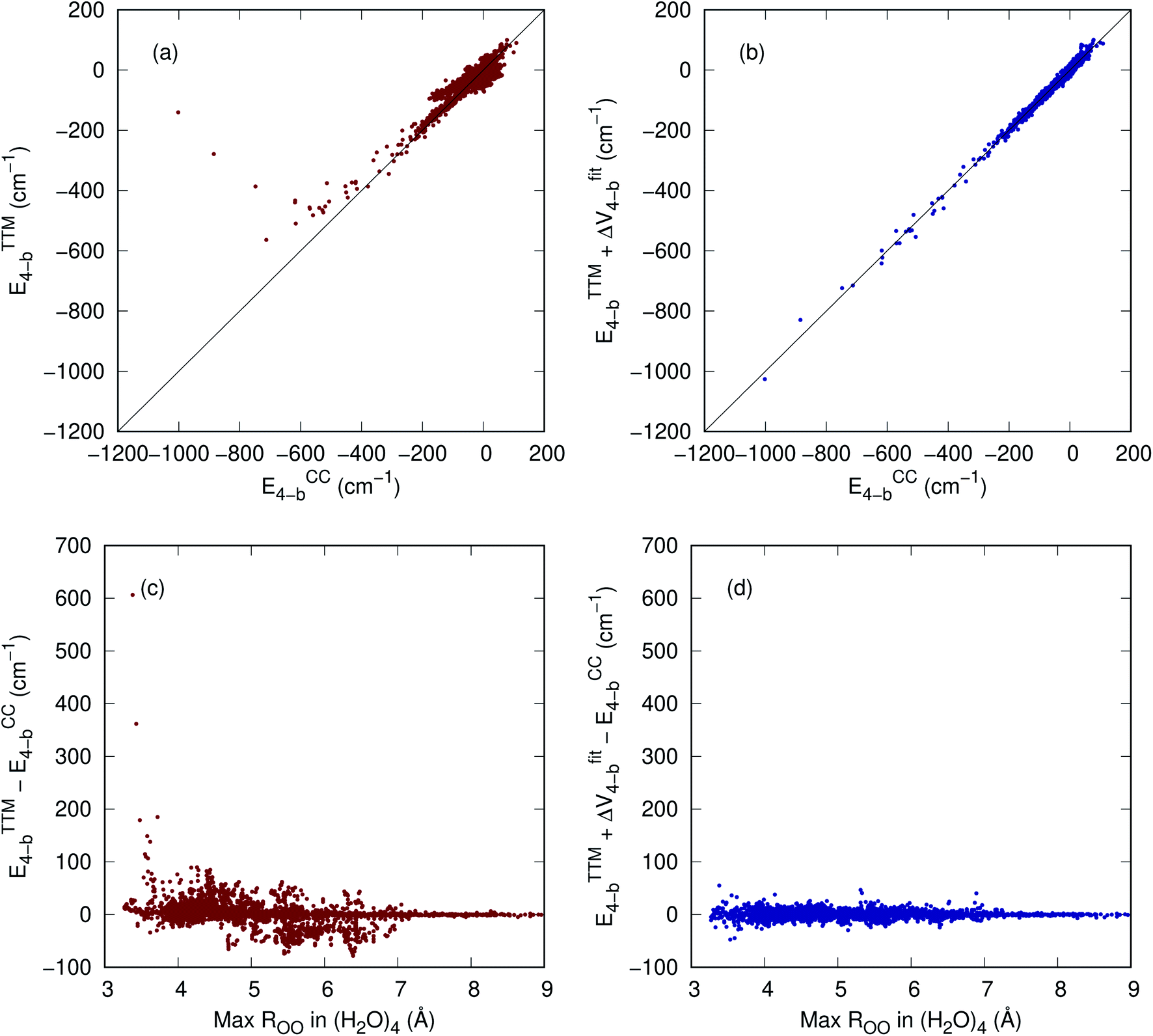Fig. 3 (a) Correlation plot between TTM4-F 4-b and CCSD(T)-F12 4-b energies; (b) correlation plot between TTM4-F + ΔV_4-b and CCSD(T)-F12 4-b energies; (c) error of TTM4-F 4-b as a function of max R_OO in the tetramer; (d) error of TTM4-F + ΔV_4-b as a function of max R_OO in the tetramer.

We now consider the binding energies of the eight isomers of the water hexamer. The binding energies for this particular water cluster have become a “benchmark” test for both electronic structure methods as well as numerous water potentials. For a recent example see ref. 29. That the hexamer has taken this central role in both theory^13,28,30,31 and experiment^32,33 is due to the fact that it is the smallest cluster with a non-planar configuration (for the O atoms). Thus, it has been termed the smallest drop of water/ice. In addition for the present purposes, this cluster has a significant number (15) of 4-b interactions. The absolute binding energies of these clusters from the benchmark electronic structure calculation (CCSD(T)/CBS values taken from ref. 28) and various PESs are listed in Table 2, and comparisons are shown in Fig. 4. As seen, with the 4-b correction, the binding energies are in better agreement with the benchmark values, especially for bag and cyclic isomers.

Table 2 Absolute binding energies (in kcal mol⁻¹) of 8 isomers of water hexamer, from CCSD(T)/CBS benchmark calculations (ref. 28) and the PESs

	CCSD(T)/CBS	MB-pol	MB-pol + ΔV4-b
Prism	45.92	45.94	45.92
Cage	45.67	45.69	45.59
Book-1	45.20	44.89	44.93
Book-2	44.90	44.68	44.70
Bag	44.30	44.03	44.19
Chair	44.12	43.66	43.82
Boat-1	43.13	42.80	42.94
Boat-2	43.07	42.82	42.96

---

Fig. 4 The binding energies of the eight isomers of the water hexamer from indicated sources.

Table 3 shows for four of the hexamer isomers the mean absolute error (MAE) in the harmonic frequencies for both uncorrected and corrected MB-pol PES. For prism and cage, the 4-b corrected version is essentially as accurate as the original MB-pol, while for book and cyclic ring, the 4-b correction clearly improves the frequencies.

Table 3 Mean absolute errors (MAE) in harmonic frequencies (in cm⁻¹) for indicated PESs. The benchmarks are from ref. 34

	Prism		Cage		Book-1		Cyclic ring
	MB-pol	+ΔV4-b	MB-pol	+ΔV4-b	MB-pol	+ΔV4-b	MB-pol	+ΔV4-b
MAE	7.8	8.4	8.9	9.4	12.6	10.6	16.5	11.7

---

Next, we comment briefly on the timing requirements for the TTM4-F + ΔV_4-b potential. As shown in the last line of Table 1, the additional time for calculating the correction for the results presented in this paper (PIP₂₀₀) is only about 1 second for 100 000 energy evaluations and approximately 3 seconds if the energy and associated gradients are evaluated at the same time. Table 4 shows the overall timing to evaluate the energy of 64, 128, and 256 monomers, with different cutoffs of the 4-b correction. In this table, t_MBX is the time to evaluate all the terms in the MB-pol, including the TTM4-F and MB-pol 2-b and 3-b, with the latest MBX software,³⁵ while t_ΔV4-b is the time to evaluate our 4-b correction term, which is the extra cost when the ΔV_4-b is added to MB-pol. All timings are evaluated using a single Intel i7-8750H core. It can be seen that the extra cost of the 4-b correction is in general a small fraction of the cost of MB-pol, and the cutoff distance can be tuned to achieve a balance between the cost and accuracy.

Table 4 Time (in seconds) needed to evaluate the energy of N_mono monomers. Here t_MBX is the time to obtain all terms in MB-pol using the latest version (MBX), and t_ΔV4-b is the time to evaluate our 4-b correction. N_tetra is the number of tetramers needed to be evaluated

N mono	t MBX	Cutoff = 6.0 Å		Cutoff = 6.5 Å		Cutoff = 7.0 Å
		N tetra	t ΔV4-b	N tetra	t ΔV4-b	N tetra	t ΔV4-b
64	0.057	1379	0.0085	2728	0.016	5639	0.032
128	0.21	5823	0.034	12 224	0.072	24 460	0.14
256	0.68	13 023	0.080	28 786	0.17	58 804	0.34

---

We have made comparisons between the TTM4-F 4-b potential, the TTM4-F 4-b with ΔV_4-b correction, and the CCSD(T) results. A remaining question that should be addressed is how the correction potential performs in comparison with the previously reported full 4-b potential¹⁵ as recently improved.¹⁶ Of course, many larger studies may already be based on the very successful MB-pol potential. For these, improvement by ΔV_4-b might be the easiest upgrade, with some extra computational cost, depending on the choice of the 4-b cutoff. But for those who are interested only in the 4-b potential, we suggest previously reported 4-b PES since it is much faster than TTM4-F 4-b + ΔV_4-b, and is slightly more accurate as well.

Finally, we note that many potentials or components of potentials can be corrected by this method, which has already been shown to be accurate and efficient for CH₄, H₃O⁺, N-methyl acetamide,⁹ and for acetylacetone,¹⁰ with more applications in process. In the current study, we have shown substantial improvement of the 4-b potential for TTM4-F, but one might have reasonable hope that this Δ-ML method is a general approach that could provide substantial improvements to other potentials at relatively small cost. In this case, the corrections would begin with the 2-b ones and could go up to 4-b. Our recent CCSD(T) 2-b, 3-b, and 4-b datasets are available,³⁶ and so the corrections, ΔV_n-b, simply require a water force field. Some examples are the well-known potentials AMOEBA,³⁷ and TTM2.1 (ref. 38) or TTM3.³⁹ These are polarizable potentials, however, with significant differences. Another force field that might be interesting to “correct” is MB-UCB.⁴⁰ Since this potential relies heavily on DFT calculation, using the ωB97X-V/def2-QZVPPD functional, it appears that the correction to MB-UCB would be analogous to the correction of DFT to CCSD(T) PESs that we considered originally in our Δ-ML method.

Summary and conclusions

The 4-b interaction in the MB-pol potential has been corrected using the proposed Δ-ML approach. The 4-b interaction itself and the correction are “small” compared to say the 2-b interaction. However, as noted above the 4-b correction has been shown to be the “ultimate” interaction by Xantheas and co-workers for large water clusters. Further it extends the successful MB-pol potential to this level of interaction. It is worth noting that the PIP fit to the difference 4-b energies is challenging because it is a 12-atom PES. While this number of atoms is not at the frontier of ML-PESs currently, it was not feasible years ago when PIP 2-b and 3-b potentials were reported for water in the WHBB⁴¹ and the MB-pol^19,20 potentials.

That the correction potential is a significant improvement over the TTM4-F potential can be seen (a) by comparing cuts of the potentials for TTM4-F 4-b, and TTM4-F 4-b + ΔV_4-b along with the CCSD(T)-F12 values; (b) by comparing the correlation between these potentials with the CCSD(T) values and the errors as a function of R_OO; (c) by comparing results for the binding energies of the water hexamer isomers; and (d) comparing the MAEs in harmonic frequencies for four of the isomers. Numerous applications of this 4-b corrected MB-pol potential can and hopefully will be done. From the present analysis, it is clear that the correction is not large; however, it does improve the accuracy of this excellent potential.

The methods described above offer three important ideas. First, we have described a method for ensuring that the potentials go to zero when appropriate distances get large. Second, we have also described a method for maintaining permutational symmetry not only in each monomer but when monomers as a whole are interchanged with one another. Finally, the ΔV method itself allows large improvements for small amount of effort, and this approach appears to be general and could be applied for other water force fields and similar types of force fields for other liquids and materials.

Data availability

The data for CCSD(T) 4-b energies and the source code for ΔV_4-b PES are available at https://github.com/szquchen/water_4b_correction/releases/tag/v1.0.

Conflicts of interest

There are no conflicts to declare.

Acknowledgements

JMB thanks the ARO, DURIP grant (W911NF-14-1-0471), for funding a computer cluster where most of the calculations were performed and current financial support from NASA (80NSSC20K0360). QY thanks Professor Sharon Hammes-Schiffer and National Science Foundation (Grant No. CHE-1954348) for support. RC thanks Università degli Studi di Milano (“PSR, Azione A Linea 2 – Fondi Giovani Ricercatori”) for support.

Notes and references

1. S. J. Pan and Q. Yang, IEEE Trans. Knowl. Data Eng., 2010, 22, 1345–1359.
2. J. S. Smith, B. T. Nebgen, R. Zubatyuk, N. Lubbers, C. Devereux, K. Barros, S. Tretiak, O. Isayev and A. E. Roitberg, Nat. Commun., 2019, 10, 2903–2906.
3. S. Käser, O. Unke and M. Meuwly, New J. Phys., 2020, 22, 055002.
4. P. Mo, M. Shi, W. Yao and J. Liu, IEEE Electron Device Lett., 2020, 41, 633–636.
5. R. Ramakrishnan, P. O. Dral, M. Rupp and O. A. von Lilienfeld, J. Chem. Theory Comput., 2015, 11, 2087–2096.
6. M. Stöhr, L. Medrano Sandonas and A. Tkatchenko, J. Phys. Chem. Lett., 2020, 11, 6835–6843.
7. M. Bogojeski, L. Vogt-Maranto, M. E. Tuckerman, K.-R. Müller and K. Burke, Nat. Commun., 2020, 11, 5223.
8. P. O. Dral, A. Owens, A. Dral and G. Csányi, J. Chem. Phys., 2020, 152, 204110.
9. A. Nandi, C. Qu, P. L. Houston, R. Conte and J. M. Bowman, J. Chem. Phys., 2021, 154, 051102.
10. C. Qu, P. L. Houston, R. Conte, A. Nandi and J. M. Bowman, J. Phys. Chem. Lett., 2021, 12, 4902–4909.
11. G. A. Cisneros, K. T. Wikfeldt, L. Ojamäe, J. Lu, Y. Xu, H. Torabifard, A. P. Bartók, G. Csányi, V. Molinero and F. Paesani, Chem. Rev., 2016, 116, 7501–7528.
12. J. P. Heindel and S. S. Xantheas, J. Chem. Theory Comput., 2020, 16, 6843–6855.
13. U. Góra, R. Podeszwa, W. Cencek and K. Szalewicz, J. Chem. Phys., 2011, 135, 224102.
14. S. K. Reddy, S. C. Straight, P. Bajaj, C. Huy Pham, M. Riera, D. R. Moberg, M. A. Morales, C. Knight, A. W. Götz and F. Paesani, J. Chem. Phys., 2016, 145, 194504.
15. A. Nandi, C. Qu, P. L. Houston, R. Conte, Q. Yu and J. M. Bowman, J. Phys. Chem. Lett., 2021, 12, 10318–10324.
16. Q. Yu, C. Qu, P. L. Houston, R. Conte, A. Nandi and J. M. Bowman, J. Phys. Chem. Lett., 2022, 13, 5068–5074.
17. B. J. Braams and J. M. Bowman, Int. Rev. Phys. Chem., 2009, 28, 577.
18. Z. Xie and J. M. Bowman, J. Chem. Theory Comput., 2010, 6, 26–34.
19. V. Babin, C. Leforestier and F. Paesani, J. Chem. Theory Comput., 2013, 9, 5395.
20. V. Babin, G. R. Medders and F. Paesani, J. Chem. Theory Comput., 2014, 10, 1599.
21. C. J. Burnham, D. J. Anick, P. K. Mankoo and G. F. Reiter, J. Chem. Phys., 2008, 128, 154519.
22. G. R. Medders, A. W. Götz, M. A. Morales, P. Bajaj and F. Paesani, J. Chem. Phys., 2015, 143, 104102.
23. MSA Software with Gradients, https://github.com/szquchen/MSA-2.0, 2021, Accessed: 2021-10-21.
24. Y. Paukku, K. R. Yang, Z. Varga and D. G. Truhlar, J. Chem. Phys., 2013, 139, 044309.
25. R. Conte, P. L. Houston and J. M. Bowman, J. Chem. Phys., 2014, 140, 151101.
26. R. Conte, C. Qu, P. L. Houston and J. M. Bowman, J. Chem. Theory Comput., 2020, 16, 3264–3272.
27. P. L. Houston, C. Qu, A. Nandi, R. Conte, Q. Yu and J. M. Bowman, J. Chem. Phys., 2022, 156, 044120.
28. D. M. Bates and G. S. Tschumper, J. Phys. Chem. A, 2009, 113, 3555–3559.
29. T. T. Nguyen, E. Székely, G. Imbalzano, J. Behler, G. Csányi, M. Ceriotti, A. W. Götz and F. Paesani, J. Chem. Phys., 2018, 148, 241725.
30. Y. M. Wang, V. Babin, J. M. Bowman and F. Paesani, J. Am. Chem. Soc., 2012, 134, 11116.
31. V. Babin and F. Paesani, Chem. Phys. Lett., 2013, 580, 1.
32. K. Liu, M. G. Brown, C. Carter, R. J. Saykally, J. K. Gregory and D. C. Clary, Nature, 1996, 381, 501–503.
33. C. Pérez, M. T. Muckle, D. P. Zaleski, N. A. Seifert, B. Temelso, G. C. Shields, Z. Kisiel and B. H. Pate, Science, 2012, 336, 897–901.
34. J. C. Howard and G. S. Tschumper, J. Chem. Theory Comput., 2015, 11, 2126.
35. MBX, https://github.com/paesanilab/MBX, 2022, Accessed: 2022-05-23.
36. 2-b, 3-b, 4-b CCSD(T) energies for water, https://github.com/jmbowma/q-AQUA, 2022, Accessed: 2022-05-22.
37. L.-P. Wang, T. Head-Gordon, J. W. Ponder, P. Ren, J. D. Chodera, P. K. Eastman, T. J. Martinez and V. S. Pande, J. Phys. Chem. B, 2013, 117, 9956–9972.
38. G. S. Fanourgakis and S. S. Xantheas, J. Phys. Chem. A, 2006, 110, 4100–4106.
39. G. S. Fanourgakis and S. S. Xantheas, J. Chem. Phys., 2008, 128, 074506.
40. A. K. Das, L. Urban, I. Leven, M. Loipersberger, A. Aldossary, M. Head-Gordon and T. Head-Gordon, J. Chem. Theory Comput., 2019, 5001–5013.
41. Y. Wang, B. C. Shepler, B. J. Braams and J. M. Bowman, J. Chem. Phys., 2009, 131, 054511.

---