
 Open Access Article
 This Open Access Article is licensed under a
 Creative Commons Attribution 3.0 Unported Licence
Exploring chemical and conformational spaces by batch mode deep active learning†
Viktor
Zaverkin
 a,
David
Holzmüller
b,
Ingo
Steinwart
b and
Johannes
Kästner
*a
a,
David
Holzmüller
b,
Ingo
Steinwart
b and
Johannes
Kästner
*a
aUniversity of Stuttgart, Faculty of Chemistry, Institute for Theoretical Chemistry, Germany. E-mail: kaestner@theochem.uni-stuttgart.de
bUniversity of Stuttgart, Faculty of Mathematics and Physics, Institute for Stochastics and Applications, Germany
First published on 12th July 2022
Abstract
The development of machine-learned interatomic potentials requires generating sufficiently expressive atomistic data sets. Active learning algorithms select data points on which labels, i.e., energies and forces, are calculated for inclusion in the training set. However, for batch mode active learning, i.e., when multiple data points are selected at once, conventional active learning algorithms can perform poorly. Therefore, we investigate algorithms specifically designed for this setting and show that they can outperform conventional algorithms. We investigate selection based on the informativeness, diversity, and representativeness of the resulting training set. We propose using gradient features specific to atomistic neural networks to evaluate the informativeness of queried samples, including several approximations allowing for their efficient evaluation. To avoid selecting similar structures, we present several methods that enforce the diversity and representativeness of the selected batch. Finally, we apply the proposed approaches to several molecular and periodic bulk benchmark systems and argue that they can be used to generate highly informative atomistic data sets by running any atomistic simulation.
1 Introduction
Recently machine-learned interatomic potentials (MLIPs) have been successfully applied to many research areas in materials science, molecular physics, and chemistry.1–5 The increasing popularity of MLIPs in the community relies mainly on their high computational efficiency, comparable to empirical force fields, and their accuracy on par with the reference ab initio methods. However, the availability of sufficiently expressive data sets, which cover the relevant part of the conformational and chemical space of interest, is a prerequisite for applying MLIPs in real-world problems.Typically, atomistic data sets employed in the literature contain thousands to millions of structures. Labels, i.e., reference energies and atomic forces, have to be computed for each of them by employing an ab initio method. The labelling is often computationally expensive. However, atomistic data sets may contain a vast amount of redundant information. For example, data sets created by employing molecular dynamics (MD) simulations generally contain many similar structures, which reduces the performance of an MLIP.
In order to reduce the required number of ab initio calculations, MLIPs can be allowed to choose which data points to label. In many situations, large sets of possible structures can easily be generated by MD simulations using a computationally cheap Hamiltonian, like force fields or preliminary trained MLIPs. An algorithm that chooses structures from such sets for which labels are to be calculated is referred to as active learning (AL).6 Such algorithms require a measure of the model's uncertainty, i.e., a criterion to decide which structures lead to the strongest increase in the quality of the training data set.
Various approaches have been proposed in the literature for Gaussian process (GP)-based MLIPs employing their Bayesian predictive variance,7–9 or the absolute error of their predictions.10 For MLIPs, which use artificial neural networks (NNs) to map atomic feature vectors to total energies, typically query-by-committee (QBC),11–14 Monte Carlo dropout,15,16 and input as well as last-layer feature space distances are used.14,16–18
Further examples are the network's output variance,19 obtained in the framework of optimal experimental design (OED),20–22 and an approach based on the D-optimality criterion proposed for linearly parameterized potentials,23 and extended later to non-linear regression.24 Finally, many AL algorithms that do not require estimating the model's uncertainty have been presented in the literature.25,26
Standard AL algorithms label one data point per iteration or choose data points independently of each other. In the construction of MLIPs, it is computationally much more efficient to provide batches of training points, for which the new labels can be calculated in parallel.6 Such batch active learning schemes reduce the computational effort arising from frequent re-training of the model, which is particularly beneficial for NN-based approaches where the training is somewhat expensive. We refer to the task of using a neural network to select multiple structures at the same time as batch mode deep active learning (BMDAL).
In order to compare AL algorithms, we consider three informal criteria that they may use to select a batch of points:27 (1) informativeness, (2) diversity, and (3) representativeness of the data. The informativeness criterion (1) requires the AL algorithm to favor structures that would be informative to the model, i.e., structures that would significantly improve the selected error measure. The informativeness could, for example, be measured by uncertainty as in ref. 19 or by the QBC approach as the disagreement among the ensemble members. The diversity criterion (2) demands that the selected samples are not too similar to each other. The last criterion (3) suggests that regions of the input space with more data points are better covered by the resulting batch. Fig. 1 compares a naive AL algorithm that fulfils (1) to algorithms that satisfy (1) and (2) or all criteria (1)–(3).
 | ||
Fig. 1 Comparison of batch mode deep active learning (BMDAL) algorithms in  feature space. (Left) The informativeness of selected structures is measured by the distance to the training points. The respective BMDAL algorithm satisfies only (1). (Middle) The data points are greedily selected28 such that the diversity of the acquired batch is enforced. The informativeness of selected structures is measured by the distance to the training and all previously selected points. In this example, the BMDAL algorithm satisfies (1) and (2). (Right) All requirements (1)–(3) are satisfied, such that the acquired batch ensures the representativity of the new training data set, defined as the union of training and newly selected data points. Here, a maximum-distance point is selected from the cluster with maximum size;29 the respective cluster centers are defined by training and previously selected points. feature space. (Left) The informativeness of selected structures is measured by the distance to the training points. The respective BMDAL algorithm satisfies only (1). (Middle) The data points are greedily selected28 such that the diversity of the acquired batch is enforced. The informativeness of selected structures is measured by the distance to the training and all previously selected points. In this example, the BMDAL algorithm satisfies (1) and (2). (Right) All requirements (1)–(3) are satisfied, such that the acquired batch ensures the representativity of the new training data set, defined as the union of training and newly selected data points. Here, a maximum-distance point is selected from the cluster with maximum size;29 the respective cluster centers are defined by training and previously selected points. | ||
Most of the methods recently presented in the literature do not satisfy all the requirements presented above. Moreover, most of them fulfil merely the informativeness criterion (1). Therefore, these methods may perform poorly on data sets containing, e.g., similar structures sampled during an MD simulation. In order to resolve these issues in the batch mode setting, here we extend existing algorithms specifically designed for BMDAL29–31 to the application on interatomic NN potentials.
Specifically, we extend the BMDAL framework proposed by ref. 29, which is explained in detail in Section 3. In this framework, to define a learned similarity measure between data points, the gradient kernel of a trained NN is considered, corresponding to the finite-width neural tangent kernel (NTK).32 Its corresponding features are the gradients of the NN output with respect to the parameters at the respective data points. In order to obtain a lower-dimensional approximation, last-layer gradient features or randomly projected gradient features are considered. The chosen kernel can then be transformed to represent uncertainties. Finally, various selection methods are presented that use kernel-based uncertainty to select a batch of data points.
We consider a specific case of atomistic NNs in which the output is defined as a sum over local atomic contributions. For the feature map corresponding to the gradient kernel, we will show that the sum over atomic contributions destroys the product structure exploited in ref. 29 for efficient exact computations. The random projections approximation from ref. 29 does not directly apply to atomistic NNs either, but we show that the linearity of individual projections in atomic features can be used to overcome this issue. As an alternative approximation, we consider the use of last-layer gradients, whose extension to atomistic NNs is straightforward and has been used recently by some of us.19 In summary, we propose random projections and last-layer gradients to efficiently approximate the full gradient kernel.
Applying the GP posterior transformation to the last-layer kernel yields an equivalent AL method to the one based on OED.19 However, in our experimental results, the application of random projections to the full gradient kernel leads to better uncertainty estimates than OED-uncertainties. Finally, various selection algorithms are introduced, ranging from the naive selection of multiple samples with the highest informativeness to more elaborated algorithms, which satisfy (1)–(3).28,29,33
To assess the performance of the proposed BMDAL methods, we thoroughly benchmark the predictive accuracy of obtained MLPs on established molecular data sets from the literature, i.e., QM9![[thin space (1/6-em)]](https://www.rsc.org/images/entities/char_2009.gif) 34–36 and MD17.37–40 Moreover, to evaluate the performance of the respective methods on bulk materials, we studied two solid-state systems, TiO241,42 and Li–Mo–Ni–Ti oxide (LMNTO).43,44
34–36 and MD17.37–40 Moreover, to evaluate the performance of the respective methods on bulk materials, we studied two solid-state systems, TiO241,42 and Li–Mo–Ni–Ti oxide (LMNTO).43,44
The software employed in this work is implemented within the TensorFlow framework45 and is published at https://gitlab.com/zaverkin_v/gmnn, including examples of usage. For MLIPs defined within the PyTorch framework,46 the reader is referred to the code published within ref. 29.
This paper is organized as follows: first, Section 2 introduces the Gaussian moment neural network (GM-NN),47,48 employed in this work for the construction of MLIPs. Then, in Section 3, we derive the gradient kernel specific to atomistic NNs, including various approximations to and the GP posterior transformation of it, and describe numerous selection algorithms designed to fulfil (1), (1) and (2), or all criteria (1)–(3). Section 4 demonstrates the performance of the proposed approaches on selected benchmark systems compared to random selection and the literature methods.10–14 Section 5 puts the main findings of this work into the context of computational chemistry and atomistic modelling in general. Finally, concluding remarks are given in Section 6.
2 Interatomic neural network potentials
In the following, the architecture and training of interatomic NN potentials employed in this work is reviewed. Throughout this work, we denote an atomic structure by , where ri are the Cartesian coordinates of atom i and
  is the respective atomic number. Particularly, we consider the problem of learning the mapping of an atomistic structure to a scalar electronic energy, i.e.
 , from data
  with
with  and
and  . Here, Erefk and
  are the reference energies and atomic forces for structure k, typically obtained by employing ab initio methods. The atomic forces are computed as negative gradients of the total energy.
Throughout this work, we employ the Gaussian moment neural network (GM-NN) approach.47,48 It allows for fast training, which is essential for training-heavy workflows such as AL. In the following, we briefly review the architecture and training of GM-NN models.
2.1 Gaussian moment neural network
In the community of NN modelling for computational chemistry, it is usual to assume that each atom interacts only with the neighbors within the finite cutoff radius rmax. Thus, the total energy of an atomistic system can be decomposed in its atomic contributions49 | (1) |
![[r with combining circumflex]](https://www.rsc.org/images/entities/b_char_0072_0302.gif) ij = rij/rij, features equivariant to rotations can be obtained as47,48
ij = rij/rij, features equivariant to rotations can be obtained as47,48 | (2) |
 is the L-fold outer product of the angular components and RZi,Zj,s(rij,β) are nonlinear radial functions with trainable parameters β. We employ a weighted sum of Gaussian functions as nonlinear radial functions,48 rescaled by the cosine cutoff function.49 Features invariant to rotations are recovered by computing tensor contractions of Cartesian tensors Ψi,L,s.47,48 When computing gradient features for BMDAL algorithms, the trainable parameters β are ignored, such that the respective algorithms can be applied similarly to other interatomic NN potentials.
We employ a fully-connected feed-forward NN consisting of two hidden layers48
 | (3) |
 for weights W(l) and 0.1 for biases b(l) for layer l. The weights of the fully-connected part are initialized by picking the respective entries from a normal distribution with zero mean and unit variance. In contrast, the trainable bias vectors are initialized to zero. We use the Swish/SiLU activation function50,51φ(x) = αx/(1 + exp(−x)) multiplied by a scalar α ≈ 1.6765 as the activation function.
To aid the training process, the output of the NN is shifted and re-scaled by trainable, species-dependent parameters μZi and σZi as
| Ei(Gi,θ) = c(σZiyi + μZi), | (4) |
2.2 Training
The parameters θ of the NN, i.e., W and b as well as the trainable parameters β of the local representation and the parameters that scale and shift the output of the NN, i.e. σZ and μZ, are optimized by minimizing the mean squared loss on training data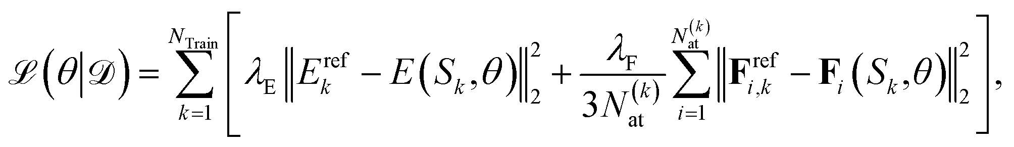 | (5) |
| Fi(Sk,θ) = −∇riE(Sk,θ). | (6) |
For the case where only reference energies are available, e.g., on the QM9 data set,34–36λF = 0 a.u. Å2 is employed.
The Adam optimizer52 is used to minimize the combined loss function in eqn (5). The respective parameters of the optimizer are β1 = 0.9, β2 = 0.999, and ε = 10−7. We employ a minibatch of 32 molecules if not stated otherwise. When training on reference energies and forces, the layer-wise learning rates were set to 0.03 for the parameters of the fully connected layers, 0.02 for the trainable representation, as well as 0.05 and 0.001 for the shift and scale parameters of atomic energies, respectively. The training was performed for 1000 training epochs. When training on reference energies only, the respective set of learning rates is 0.005, 0.0025, 0.05, and 0.001, respectively. In this case, the model was trained for 500 epochs. To prevent overfitting during training, we employed the early stopping technique.53
All models were trained within the TensorFlow framework45 on a central processing unit (CPU) node equipped with two Intel Xeon E6252 Gold (Cascade Lake) CPUs. For all tests performed in this work, eight models were trained in parallel on a single CPU node, i.e. six cores were used by a process.
3 Active learning
All BMDAL approaches considered here require an estimate of the informativeness of a queried point to the model. Here, we are interested in BMDAL approaches which are able to select a diverse set , with Nbatch > 1 at once from the unlabeled pool of data
  . We employ the framework proposed by ref. 29. Thus, BMDAL methods will be defined through base kernels representing some measure of similarity and importance on the data, transformations of the base kernels and selection methods using the transformed kernels.
Here, the framework mentioned earlier29 is extended to the application of interatomic NN potentials. Therefore, a thorough derivation of all components is required. In the following, we introduce the positive semi-definite kernel  , defined by a finite-dimensional feature map
  as
as
| k(S,S′) = ϕ(S)Tϕ(S′), | (7) |
 being a set of structures and dfeature being the dimensionality of the feature space. For more information on kernels, the reader is referred to ref. 54.
Only the energy output is considered in this section, provided directly by the model. The atomic forces are neglected as they are defined by a negative gradient of the total energy. Additionally, for the last-layer gradient approximation, it has been demonstrated that the informativeness defined by atomic forces is only marginally more expressive than the one obtained by the energy-based approaches.19 Moreover, the computational demand of atomic force-based approaches is far greater than that of total-energy-based ones. An exception are the reference literature methods such as QBC and those based on absolute errors.10–14
3.1 Kernels as measures for similarity and uncertainty
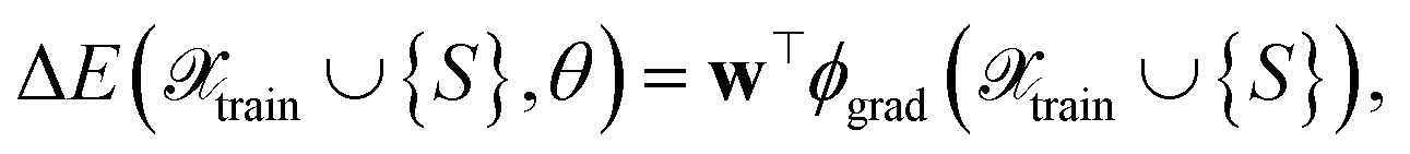
In the following, we will discuss several ways to define kernels as similarity and uncertainty measures for NN models, which will be combined with different selection methods. We expect trained NNs to learn better measures of similarity between points and, therefore, lead to better uncertainty estimates for the NN. To be able to refer to them in Section 4, we now assign labels to them, like FEAT(LL) for the similarity measured as the distance between last-layer gradient feature vectors. We will do this by first considering various base kernels and then various transformations thereof.| E(S,θ) ≈ E(S,θ*) + wT∇θE(S,θ)|θ=θ*, | (8) |
 | (9) |
 as the difference between reference labels and predictions
  .
.
The kernel kgrad(S,S′) = ϕgrad(S)Tϕgrad(S′) corresponds to the finite-width NTK,32 and depends on the linearization point θ*. In the infinite width limit, i.e. dl → ∞ for 1 ≤ l ≤ L − 1, it can converge to a deterministic limit.32,55–57 For this work, however, it is essential that NTK governs the training of NN-based models, at least in the first-order Taylor approximation. Thus, it contains relevant information on the informativeness of queried samples. Then, for example, the distances between the respective feature vectors
 | (10) |
We recall that a sum of atomic contributions models the total energy of a system. Therefore, the feature map ϕgrad(S) can also be decomposed into the atomic contributions ϕgrad(Gi), i.e. one can write
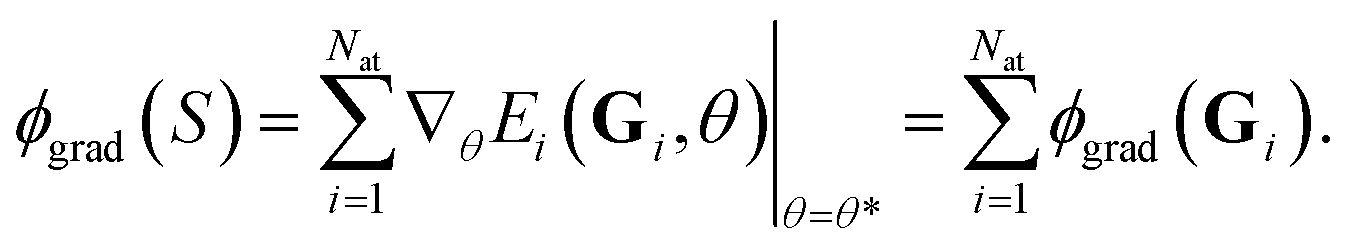 | (11) |
Formally, ϕgrad(Gi) can be easily computed by employing its product structure. For this purpose, we rewrite the network in eqn (3) as29
 | (12) |
 | (13) |
The product structure of ϕgrad in eqn (13) will be essential in Section 3.1.3.
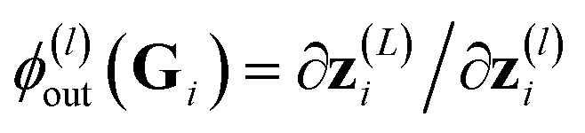
ϕll(S) = ∇![[W with combining tilde]](https://www.rsc.org/images/entities/b_char_0057_0303.gif) (L)E(S,θ), (L)E(S,θ), | (14) |
referred to as network's sensitivity in ref. 19. Similar features are frequently used in the literature.16,28 In Section 4, we will refer to the respective kernel, i.e. k(S,S′) = ϕll(S)Tϕll(S′), as to FEAT(LL).
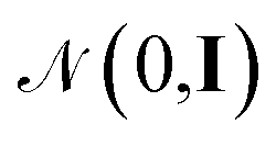
For a general feature map ϕ(Gi) ∈ ![[Doublestruck R]](https://www.rsc.org/images/entities/char_e175.gif) dfeature and a random matrix
dfeature and a random matrix  with drp being the number of random projections, we can consider the randomly projected feature map
 | (15) |
 | (16) |
For the random feature map ϕrpgrad(Gi) one obtains by employing the expressions in eqn (16)
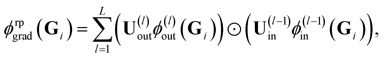 | (17) |
 and ϕ(l)in(Gi) =
 ![[x with combining tilde]](https://www.rsc.org/images/entities/b_char_0078_0303.gif) (l)i. All U(l)in and U(l)out are sampled independently.
(l)i. All U(l)in and U(l)out are sampled independently.
In contrast to ref. 29, we cannot directly use eqn (17), since we need to work with a sum 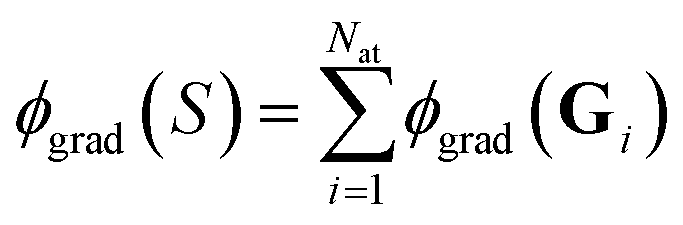 of atomic gradient features. In order to apply the random projections from eqn (17) to a sum of features, we note that the individual projections (rows of eqn (17)) are linear in the features ϕgrad(Gi)
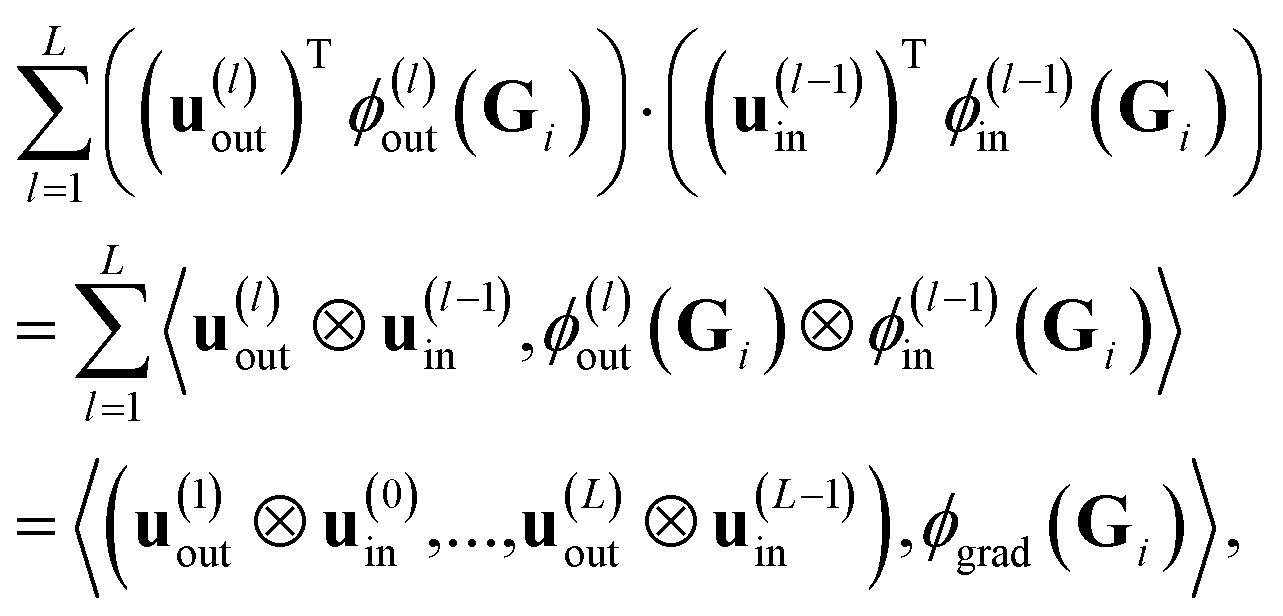 | (18) |
Given the linearity in eqn (18), we can apply random projections to a sum of feature maps simply by summing the individual random projections, given that all of the individual random projections use the same random matrices. Specifically, we obtain for the feature map of a structure S
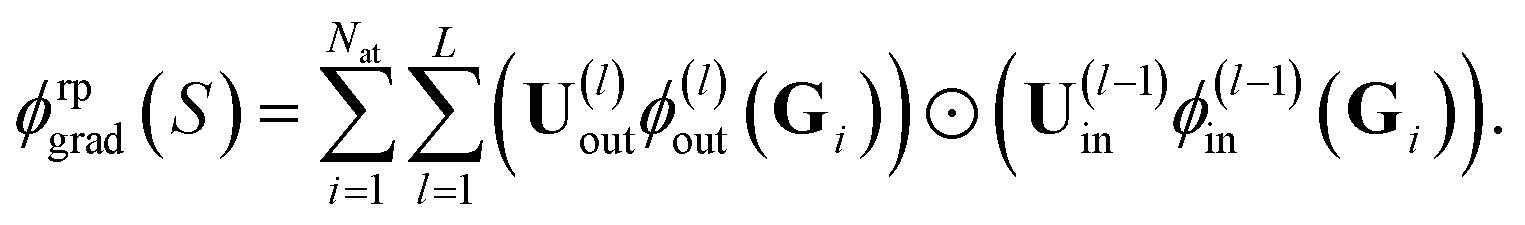 | (19) |
These random projections gradient features can be used when computing the distance between two structures (similarity) in the respective feature space, see eqn (10). In Section 4, we will refer to the respective kernel, i.e., k(S,S′) = ϕrpgrad(S)Tϕrpgrad(S′), as FEAT(RP). Alternatively, one can obtain the variance at a queried point and the covariance between queried points by computing the GP posterior on k(S,S′).
 . The energy is then modeled by
| E(S,θ) = wTϕ(S) + ε, | (20) |
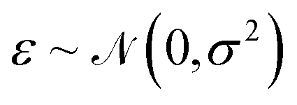 is the observation noise and wTϕ(S) is the random function with covariance defined by eqn (7). After observing the training data
  one obtains again a Gaussian process with the well-known covariance kernel7
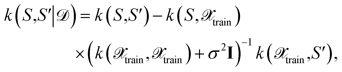 | (21) |
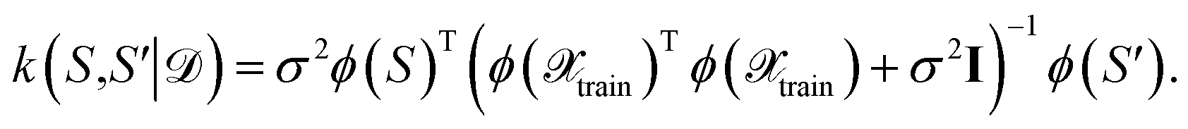 | (22) |
Thus, one may define a GP posterior transformed feature map as
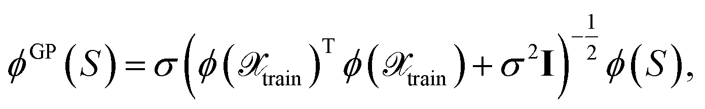 | (23) |
which can be used to estimate the informativeness of a queried point by eqn (10). In Section 4, we refer to the kernel in eqn (22) or (21) as GP(LL) and GP(RP) if last-layer or random projections gradient features have been used, respectively. Similar to the scaling transformation in ref. 29, we choose σ2 in a data-dependent fashion as 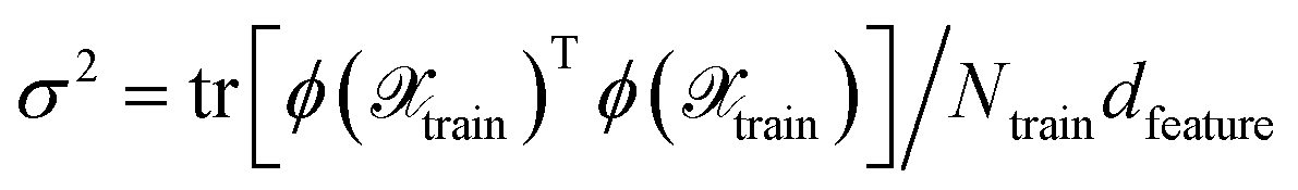 .
.
As an alternative to the distance-based measure of informativeness in eqn (10), after the GP posterior transformation the uncertainty of the network is given by the diagonal elements of the kernel in eqn (21), i.e.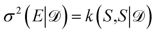 , which is equivalent to the results obtained in the OED framework,19 if last-layer gradient features are used. A naive BMDAL approach would select Nbatch samples with the highest uncertainty.19 However, the off-diagonal elements of kernel in eqn (21) and (22) describe the cross-correlation of structures S and S′ and can be used to obtain BMDAL methods satisfying (1) and (2); see Section 3.2.2.
 | (24) |
respectively. Then, the respective kernels are defined as k(S,S′) = ΔE(S)δS,S′ or k(S,S′) = ΔF(S)δS,S′. In Section 4, we will refer to the abovementioned kernels as AE(E) and AE(F), respectively.
Alternatively, for the QBC approach, we define the disagreement between ensemble members by
 | (25) |
for total energies and atomic forces, respectively. Here, Nens is the number of models in the ensemble,  and
and  are the mean of the respective property prediction. The corresponding kernels are defined by k(S,S′) = σensE(S)δS,S′ or k(S,S′) = σensF(S)δS,S′. These kernels will be called QBC(E) and QBC(F), respectively. Throughout this work, we employed an ensemble of three models. For all numerical results in Section 4, we report the average errors over the individual models in the ensemble.
Finally, one can model random selection by a diagonal kernel with k(S,S′) = uSδS,S′ with uS drawn i.i.d. from, e.g., a uniform distribution. We refer to this random kernel as RND.
3.2 Selection methods
Given an appropriate measure of informativeness, one has to define particular selection methods. Here, we describe various selection methods. Some of them satisfy only the informativeness criterion (1). Others ensure the diversity of the acquired batch (2) and the representativeness of the updated training set (3). An efficient algorithmic realization of the selection methods discussed in this section has been used for our implementation but is not discussed here; for more details, see Appendix D of ref. 29. we select the next point by
 | (26) |
until Nbatch structures are selected. Combined with the GP(LL) kernel, we obtain the method previously derived within the OED framework.19 The selection method in eqn (26) (or MAXDIAG in the following) can be combined with all kernels described in Section 3.1.5 resembling most of the literature methods.10–14 However, MAXDIAG satisfies only the informativeness criterion (1) and do not enforce batch diversity or the representativeness criteria. Therefore, it may select similar structures which would deteriorate performance of an MLIP.
 | (27) |
The above expression is equivalent to the BatchBALD approach proposed for classification problems,33 if applied to a GP model.29 A naive implementation of eqn (27) would require computing each determinant separately. In this work, we employ the greedy algorithm proposed by ref. 59 and described in ref. 29, which uses the partial pivoted matrix-free Cholesky decomposition.59 We call the corresponding selection method MAXDET, which corresponds to MAXDET-P in ref. 29. MAXDET satisfies (1) and (2) but does not take the distribution of the pool data (3) into account.
In ref. 29, it was assumed that the training and pool labels are corrupted with Gaussian noise. In this work, the labels are generated by ab initio methods and are assumed to be noise-free. Therefore, compared to ref. 29, we skip the label noise in eqn (27), i.e., we maximize  instead of
 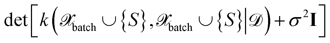 . This modification additionally ensures that the same input cannot be queried multiple times in the same batch. On the other hand, it also means that MAXDET can select at most dfeature batch elements in a BMDAL step, since the determinant in eqn (27) becomes zero afterwards. In contrast, the distance-based methods defined below can select a batch of arbitrary size.
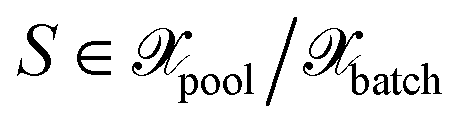
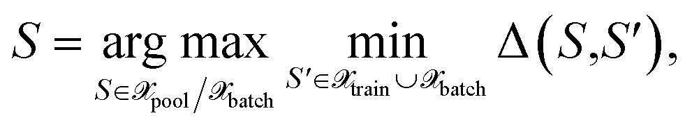 | (28) |
with the distance measure defined in eqn (10) but employing the selected kernel. Originally, the approach defined by eqn (28) was proposed for classification tasks.28 Some examples of the usage of distances in the feature space are known also for MLIPs,16 but they are restricted to measuring the distance to all training points as shown in Fig. 1 (left). Here, we are dealing with a greedy distance optimization as in Fig. 1 (middle), instead. We call the corresponding selection methods as MAXDIST, which corresponds to MAXDIST-TP in ref. 29. Similar to MAXDET, MAXDIST satisfies (1) and (2) but does not take the distribution of the pool data (3) into account.
 we define the associated center as
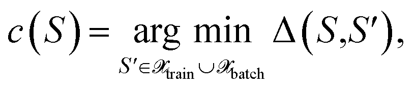 | (29) |
with the distance measure as defined by eqn (10). Then, for each center  the cluster size is defined as the sum over squared distances from the cluster center to all points in the cluster
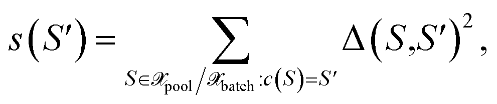 | (30) |
i.e., for all points S for which c(S) = S′ holds. Finally, among all points from the cluster with maximum size, the most distant point from the respective cluster center is selected
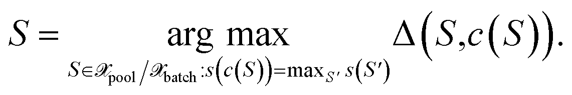 | (31) |
We should note that the LCMD approach can be disadvantageous compared to MAXDIST and MAXDET if the pool data is not representative for the test data or if the maximum error is important.29
4 Results
In the following, methods and algorithms presented in this work are applied to learning interatomic potentials, specifically to GM-NN models;47,48 see Section 2. We employ four benchmark data sets. The MD17 data set37–40 covers the sampling of the conformational space, while QM934–36 covers the sampling of the chemical space. Moreover, we investigate the applicability of the proposed approaches on bulk materials by employing the TiO241,42 and LMNTO data sets.43,44
We have employed 15 BMDAL algorithms obtained by combining selection and kernel methods discussed in Section 3. These are:
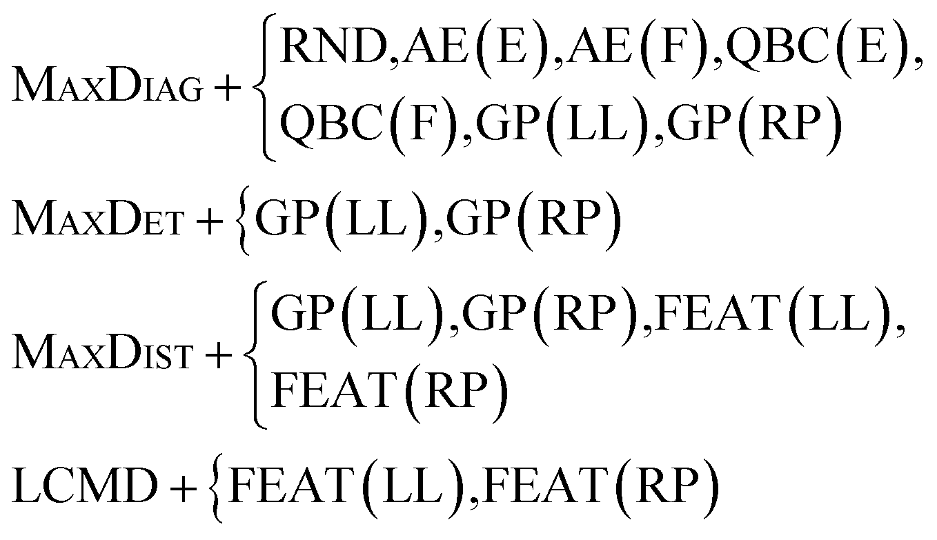
The chosen combinations of selection methods and kernels are motivated as follows: MAXDIAG + RND performs random selection and is used as a baseline. The MAXDIAG + QBC and MAXDIAG + GP methods correspond to conventional AL methods.10–14,19 The MAXDIAG + AE methods show what is possible with AL when labels on the pool set are available. The combinations MAXDET + GP, MAXDIST + FEAT, and LCMD + FEAT are motivated by ref. 29. We include MAXDIST + GP as an additional experiment.
In total, we ran 292 BMDAL experiments that were repeated five times with different seeds for NN initialization and splitting data into training, validation, pool, and test data sets. In total, 69154 models have been trained. However, as it is infeasible to visualize all the results in this section, only the most illustrative results are presented. For more details (including the numerical values for the selected experiments), the reader is referred to the ESI.†
4.1 Sampling conformational space
Probably the most appropriate benchmark data for BMDAL presented in the literature is the MD17 data set,37–40 which contains 150000 to almost 1000000 conformations of each of eight small organic molecules. The data set includes structures, energies, and atomic forces of the respective conformations. Here, we decided to use only the aspirin molecule data, while similar results are expected for the other molecules contained in MD17. As a cutoff radius we selected a value of rmax = 4.0 Å.47 The respective data was sampled from ab initio molecular dynamics (AIMD) simulations. Given many conformations, we expect most of them to be similar. Thus, methods that ignore diversity (2) may lead to worse performance of actively learned GM-NN potentials than those trained on randomly selected samples.
The aspirin data set contains structures, energies, and atomic forces of 211762 conformations; 150000 were reserved as pool data. Depending on the specific BMDAL scenario, we began by training the GM-NN model on 10 or 100 samples drawn randomly from the data set. Additionally, we reserve 2000 structures for validation, which are used for early stopping. We hold back the remaining 59752 and 59662 conformations for testing the GM-NN models, respectively. In each BMDAL step, the training data set is increased by a batch size of Nbatch = {2, 5, 10} or Nbatch = {10, 25, 50, 100} structures, until a maximum size of 100 and 1000 has been reached, respectively. For brevity we refer to the respective BMDAL experiments as (10, 100; {2, 5, 10})MD17 and (100, 1000; {10, 25, 50, 100})MD17. Here, the results for the former are discussed in more detail. For the results on (100, 1000; {10, 25, 50, 100})MD17 the reader is referred to the ESI.†
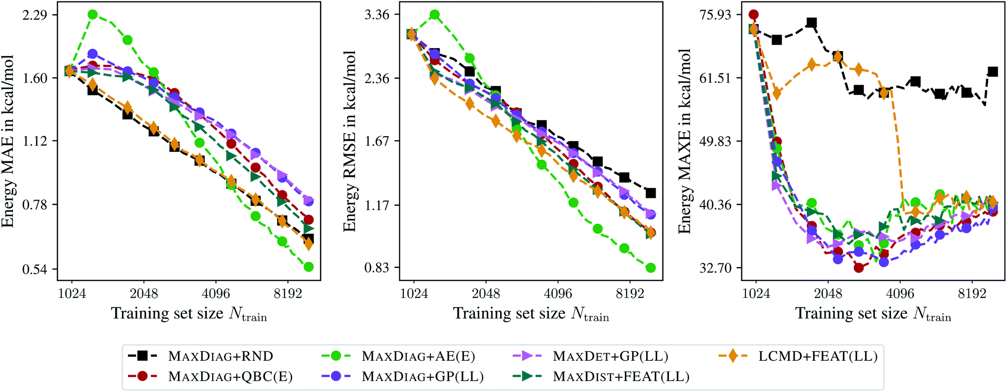
Fig. 2 shows the dependence of the mean absolute errors (MAE), root-mean-square errors (RMSE), and maximum errors (MAXE) on the acquired batch size Nbatch for atomic forces. The respective plots for total energies can be found in the ESI.† From Fig. 2 one can observe that GM-NN models trained via BMDAL algorithms that ignore (2), i.e., MAXDIAG + QBC(F), MAXDIAG + AE(F), MAXDIAG + GP(LL), perform worse than those trained on randomly selected data, MAXDIAG + RND. Moreover, their MAE, RMSE, and MAXE increase with increasing size of the acquired batch. By contrast, the BMDAL methods that enforce diversity (2), i.e., MAXDET + GP(LL) and MAXDIST + FEAT(LL), or diversity (2) and representativeness (3), i.e., LCMD + FEAT(LL), improve the performance of GM-NN models compared to random selection.
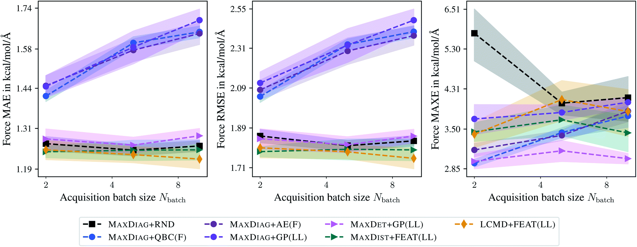 | ||
| Fig. 2 Dependence of the mean absolute errors (MAE), root-mean-square errors (RMSE), and maximum errors (MAXE) of atomic forces on the acquired batch size Nbatch. All errors are evaluated for the last BMDAL step on the aspirin molecule data from MD17.37–40 Shaded areas denote the standard error on the mean evaluated over five independent runs. | ||
Fig. 3 demonstrates the learning curves for the selected BMDAL methods. All results are presented for the maximal acquired batch size of Nbatch = 10. From Fig. 3, we can see that the BMDAL methods that satisfy at least (1) and (2) outperform random selection over the course of BMDAL. The MAXDIAG-based methods lead to results worse than those obtained for models trained on randomly selected data. We found for LCMD + FEAT(LL), the best performing BMDAL method in terms of MAE and RMSE, 1.22, 1.75, and 3.83 kcal mol−1 Å−1 for force MAE, RMSE, and MAXE, respectively. By contrast, for random selection we obtained 1.26, 1.83, and 4.12 kcal mol−1 Å−1, respectively. MAXDIST + FEAT(LL) and MAXDET + GP(LL) appear to outperform LCMD + FEAT(LL) in terms of MAXE with 3.43 and 3.00 kcal mol−1 Å−1, respectively. All results are given for Ntrain = 100 training samples. While the achieved MAE in atomic forces still exceeds the desired accuracy of 1 kcal mol−1 Å−1, this can be resolved by selecting slightly more data points, as demonstrated in Fig. 5 in the ESI.†
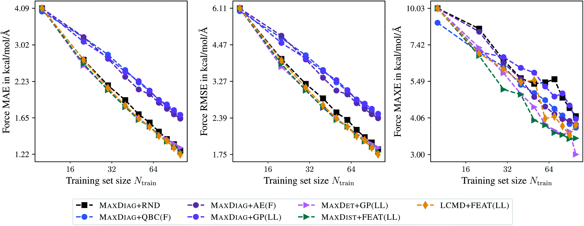 | ||
| Fig. 3 Learning curves for the aspirin molecule data from MD17.37–40 The mean absolute errors (MAE), root-mean-square errors (RMSE), and maximum errors (MAXE) of atomic forces are plotted against the training set size acquired during BMDAL. The training errors before the first BMDAL step are identical for most methods since they use the same random seed. This does not apply to QBC, where more models are trained. Results obtained for larger data set sizes can be found in the ESI.† | ||
Besides the last BMDAL step, we analyze MAE, RMSE, and MAXE averaged over the learning curve in order to investigate the general learning behavior. Here, MAXDIST + FEAT(LL) with 1.90, 2.78, and 4.86 kcal mol−1 Å−1, respectively, appears to be the best performing BMDAL strategy. MAXDET + GP(LL) slightly outperforms LCMD + FEAT(LL), especially in terms of MAXE with 5.02 and 5.33 kcal mol−1 Å−1, respectively. For comparison, we find for random selection 1.96, 2.89, and 6.04 kcal mol−1 Å−1 in predicted atomic forces. We observe that AL approaches are especially beneficial for MAXE and less so for MAE. This is in line with our previous observations.19,29
Concerning the computational demand, random selection is certainly advantageous compared to any BMDAL method since it does not require any additional computational steps. Thus, to motivate the presented BMDAL methods, we compare them to the QBC approach. For MAXDIAG + QBC(F) we obtained 280 s for evaluating the respective features. The evaluation of gradient features requires less time by a factor of 3 to 4, even neglecting the fact that it only required to train a single model. Another important criterion is the time used to select the batch of structures. While MAXDIAG + QBC(F) selects the batch in 0.00–0.03 s, MAXDET + GP(LL) and LCMD + FEAT(LL) require 0.89 and 4.65 s, respectively. Thus, the proposed BMDAL methods, i.e., those based on gradient features and selection methods which enforce (2) or (2) and (3), are still much more time-efficient than literature methods.10–14 We should note that MAXDIAG + AE(F) would require much more time since it would require performing ab initio calculations for all structures in the pool. All times are obtained when running eight processes in parallel on two Intel Xeon E6252 Gold (Cascade Lake) CPUs.
Now we compare the last-layer with random projections of gradient kernels. For this purpose, we plot MAE, RMSE, and MAXE for the last BMDAL step against the acquired batch size Nbatch, similar to Fig. 2. Fig. 4 demonstrates that in most cases, BMDAL methods which estimate the informativeness of structures by the random projections gradient kernel outperform those which use the last-layer gradient one, similar to ref. 29. Additionally, we observed an improved correlation of the uncertainty with the actual error: the linear correlation or Pearson correlation coefficient (PCC) for MAXDET + GP(RP) and MAXDET + GP(LL) are 0.47 and 0.23, respectively. We note that computing random projections gradient features are computationally more demanding than the last-layer ones. However, the difference is only about a factor of 1.31. For MAXDET + GP(LL) the feature matrix was computed during 66.54 s, while for MAXDET + GP(RP) it required 87.37 s. All times are obtained when running eight processes in parallel on two Intel Xeon E6252 Gold (Cascade Lake) CPUs.
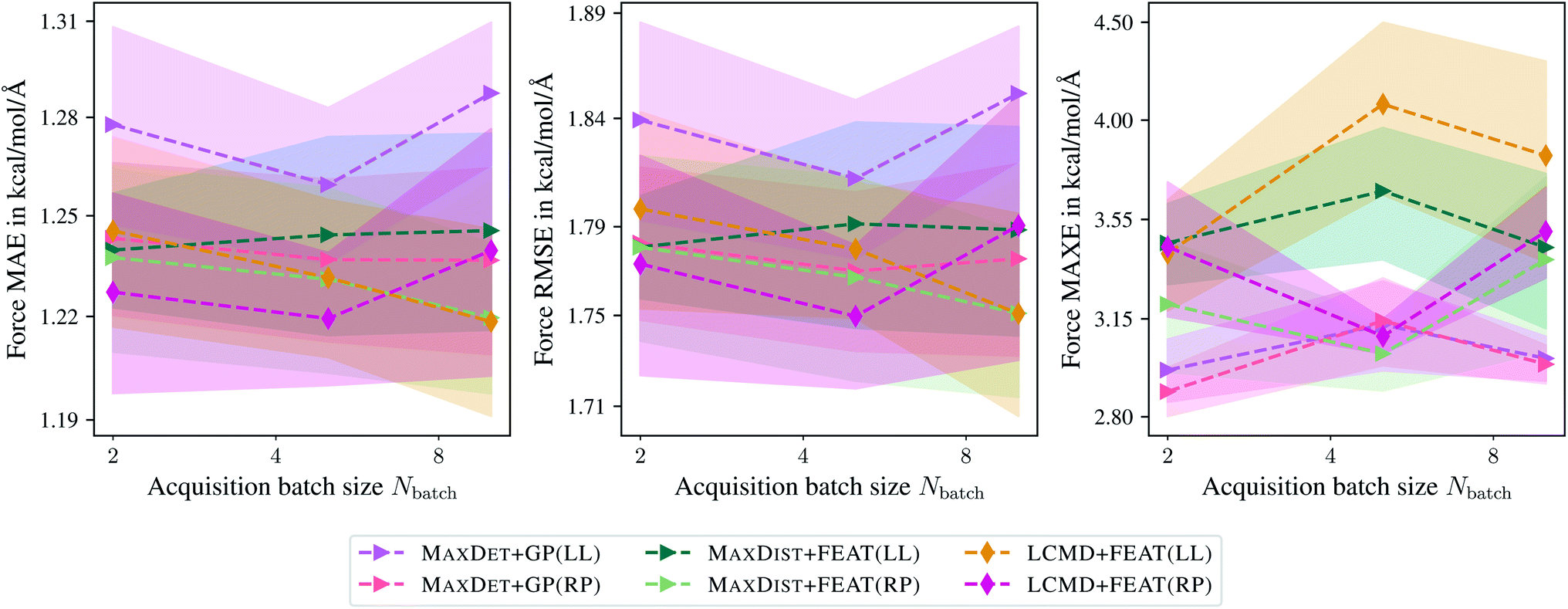 | ||
| Fig. 4 Comparison of the last-layer and random projections gradient feature maps on the aspirin molecule data from MD17.37–40 The mean absolute errors (MAE), root-mean-square errors (RMSE), and maximum errors (MAXE) of atomic forces are plotted against the acquired batch size Nbatch. Shaded areas denote the standard error on the mean evaluated over five independent runs. | ||
4.2 Sampling chemical space
The QM9 data set34–36 contains several properties of molecules in equilibrium, i.e., all forces vanish. Here, we are interested in predicting atomization energies. In total, the QM9 data set consists of 133885 neutral, closed-shell organic molecules with up to 9 heavy atoms (C, O, N, F) and a varying number of hydrogen (H) atoms. As 3054 molecules from the original QM9 data set failed a consistency test,35 we used only the remaining 130831 structures in the following. For the QM9 data set, we used a cutoff radius of rmax = 3.0 Å.47,48 The application of BMDAL methods to QM9 can be seen as an application to the sampling of the chemical space.
For all BMDAL experiments, we reserve 100000 molecules for the unlabeled pool. Depending on the specific BMDAL scenario, the GM-NN model is initialized by training on 1000 or 5000 samples drawn randomly from the data set. Additionally, we reserve 2000 structures for validation. We hold back the remaining 27831 and 23831 molecules for testing the GM-NN models, respectively. In each BMDAL step, the training data set is increased by a batch size of Nbatch = {50, 100, 250} or Nbatch = 250 molecules, until a maximum size of 10000 or 25000 has been reached, respectively. For brevity we refer to the respective BMDAL experiments as (1000, 10000; {50, 100, 250})QM9 and (5000, 25000; 250)QM9. Here, the results for the former are discussed in more detail. For the results on (5000, 25000; 250)QM9 the reader is referred to the ESI.†
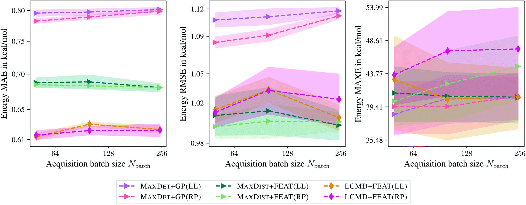
Fig. 5 shows the dependence of MAE, RMSE, and MAXE of the atomization energies on the acquired batch size Nbatch. From Fig. 5 one can observe that only LCMD + FEAT(LL) and MAXDIAG + AE(E) could improve on the MAE compared to random selection. However, we see a considerable improvement for all methods for RMSE and MAXE, although no improvement over literature MAXDIAG + QBC(E) methods could be achieved. MAXDIAG + GP(LL) provides similar results to those of MAXDET + GP(LL). MAXDIAG + AE(E) provides the best results in terms of MAE and RMSE. This observation can be explained by the high diversity of molecules in the QM9 data set. In summary, all considered BMDAL approaches are relatively successful on this kind of data.
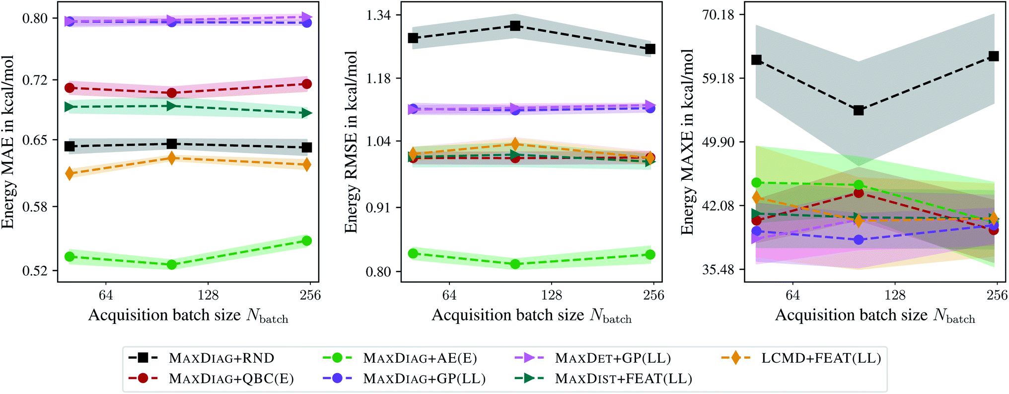 | ||
| Fig. 5 Dependence of the mean absolute errors (MAE), root-mean-square errors (RMSE), and maximum errors (MAXE) of the atomization energies on the acquired batch size Nbatch. All errors are evaluated for the last BMDAL step on the QM9 data set.34–36 Shaded areas denote the standard error on the mean evaluated over five independent runs. | ||
Fig. 6 presents the learning curves for the QM9 data set obtained for the maximum acquired batch size of Nbatch = 250. From Fig. 6 one can observe that only LCMD + FEAT(LL) and MAXDIAG + AE(E) can improve on the MAE compared to random selection. Moreover, LCMD + FEAT(LL) considerably outperforms MAXDIAG + AE(E) for Ntrain ≲ 2048. We note that MAXDIAG + AE(E) requires computing labels on the pool data and is not tractable in a practical setting. From Fig. 6 one can see that all proposed AL methods improve on RMSE and MAXE compared to random selection, similar to the results by ref. 19. For LCMD + FEAT(LL) and Ntrain = 10000, we obtained MAE, RMSE, and MAXE of 0.62, 1.01, and 40.67 kcal mol−1, respectively. By contrast, for random selection we found 0.64, 1.25, and 62.77 kcal mol−1, respectively.
 | ||
| Fig. 6 Learning curves for the QM9 data set.34–36 The mean absolute errors (MAE), root-mean-square errors (RMSE), and maximum errors (MAXE) of the atomization energies are plotted against the training set size acquired during BMDAL. The markers show only a subset of all BMDAL steps for better visibility, while the lines use all steps. The training errors before the first BMDAL step are identical for most methods since they use the same random seed. This does not apply to QBC, where more models are trained. | ||
Interestingly, for (5000, 25000; 250)QM9 no improvement in terms of MAXE could be observed, different from ref. 19, while RMSE is reduced considerably by employing BMDAL. The observed behavior may be attributed to the improvements introduced to the GM-NN approach in ref. 48 or to the fact that ref. 19 used the remaining pool data as the test data, which is more realistic if BMDAL is run in an on-the-fly fashion. For LCMD + FEAT(LL) and Ntrain = 25000 we obtained 0.40, 0.71, and 35.85 kcal mol−1 for MAE, RMSE, and MAXE, respectively. We obtained 0.43, 0.92, and 38.61 kcal mol−1 for random selection, respectively.
The selection time is another important criterion when deciding which particular BMDAL method should be used. For example, while the QBC features requires about 46 s for the calculation, the naive selection algorithm in Section 3.2.1 needs only a few milliseconds. By contrast, the last-layer features in LCMD + FEAT(LL) required 27.35 s for the evaluation. However, the corresponding selection method is much more demanding and needs 180.74 s. The total time required by the MAXDET + GP(LL) strategy equals 40.46 s, which makes it advantageous compared to LCMD + FEAT(LL). All times are obtained when running eight processes in parallel on two Intel Xeon E6252 Gold (Cascade Lake) CPUs.
Finally, we compare the last-layer and random projections gradient kernels employed for the uncertainty estimation. Fig. 7 indicates that random projections gradient kernel may lead to a slight improvement over the last-layer gradient kernel. At the same time, only minor differences in computational demand have been observed; computing the feature matrix takes 27.35 s and 38.32 s for LCMD + FEAT(LL) and LCMD + FEAT(RP), respectively. A slight improvement in measured PCC could be observed; 0.22 and 0.26 for MAXDET + GP(LL) and MAXDET + GP(RP), respectively.
 | ||
| Fig. 7 Comparison of the last-layer and random projections gradient feature maps on the QM9 data set.34–36 The mean absolute errors (MAE), root-mean-square errors (RMSE), and maximum errors (MAXE) of the atomization energies are plotted against the acquired batch size Nbatch. Shaded areas denote the standard error on the mean evaluated over five independent runs. | ||
4.3 Bulk materials
Now we apply the proposed BMDAL methods to two bulk systems: TiO241,42 and Li–Mo–Ni–Ti oxide (LMNTO).43,44 The former contains Cartesian coordinates, energies, and atomic forces of distorted rutile, anatase, and brookite structures. Moreover, the configurations sampled from short AIMD simulations and supercell structures with oxygen vacancies are included. In total, the TiO2 data set contains 7815 structures ranging in size from 6 to 95 atoms per unit cell. The LMNTO data set contains 2616 Cartesian coordinates, energies, and atomic forces extracted from a 50 ps long AIMD simulation at 400 K. Each structure in the LMNTO data set consists of 56 atoms (Li8Mo2Ni7Ti7O32). For both data sets we used a cutoff radius of rmax = 6.5 Å.48
For the TiO2 data set, we reserved 6000 structures for the pool data. Depending on the specific scenario, the initial training set contained 10 or 500 structures. Additionally, we reserve 200 structures for validation. We hold back the remaining 1605 and 1115 structures for testing the GM-NN models obtained during BMDAL runs. In each BMDAL step, the training data set is increased by a batch size of Nbatch = {2, 5, 10} or Nbatch = {50, 100, 250} molecules, until a maximum size of 100 or 2500 has been reached, respectively. For the LMNTO data set, we reserved 100, 200, and 2000 structures for the training, validation, and pool data. The remaining 316 structures were used to test the resulting GM-NN models. For brevity we refer to the respective BMDAL experiments as (10, 250; {2, 5, 10})TiO2, (500, 2500; {50, 100, 250})TiO2, and (100, 1000; {25, 50, 100})LMNTO, respectively. Here, the results for (10, 250; {2, 5, 10})TiO2 and (100, 1000; {25, 50, 100})LMNTO are discussed in more detail. For the results on (500, 2500; {50, 100, 250})TiO2 the reader is referred to the ESI.†
Fig. 8 and 9 show the dependence of MAE, RMSE, and MAXE in atomic forces on the acquired batch size Nbatch on the TiO2 and LMNTO data sets. The respective plots for total energies can be found in the ESI.† From Fig. 8 one can observe that for RMSE and MAXE, the application of any BMDAL method leads to a considerable improvement over random selection. This observation is consistent with the fact that unlike MD17, where all data was obtained by running AIMD, the TiO2 data set contains many diverse structures. For MAE, the dependence on the batch size can be observed for methods that do not satisfy the diversity criterion (2). MAXDET + GP(LL), MAXDIST + FEAT(LL), and LCMD + FEAT(LL) improve on MAE and the results are independent of the acquired batch size. Similar results for MAE and RMSE are obtained for the LMNTO data set; see Fig. 9. However, no improvement could be achieved for MAXE as the data set most probably does not contain any strongly distorted structures. We decided to skip LMNTO in the following discussion.
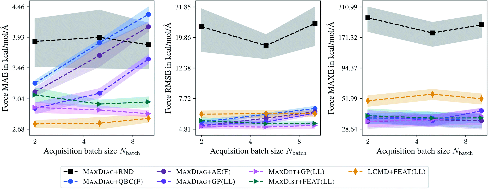 | ||
| Fig. 8 Dependence of the mean absolute errors (MAE), root-mean-square errors (RMSE), and maximum errors (MAXE) of atomic forces on the acquired batch size Nbatch. All errors are evaluated for the last BMDAL step on the TiO2 data set.41,42 Shaded areas denote the standard error on the mean evaluated over five independent runs. | ||
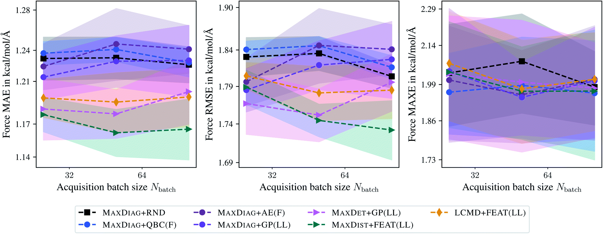 | ||
| Fig. 9 Dependence of the mean absolute errors (MAE), root-mean-square errors (RMSE), and maximum errors (MAXE) of atomic forces on the acquired batch size Nbatch. All errors are evaluated for the last BMDAL step on the LMNTO data set.43,44 Shaded areas denote the standard error on the mean evaluated over five independent runs. | ||
Fig. 10 shows learning curves obtained for the TiO2 data set and an acquired batch size of Nbatch = 10. We can observe a considerable improvement of BMDAL methods which enforce at least (2) over naive or random selection. The GM-NN models trained by BMDAL methods required only about half of the structures to reach the same RMSE value as MAXDIAG-based approaches. For example, for MAXDET + GP(LL) we obtained an RMSE of 17.43 kcal mol−1 Å−1 for Ntrain = 30, while an RMSE of 17.71 kcal mol−1 Å−1 for Ntrain = 60 was found for MAXDIAG + GP(LL). For MAXE in atomic forces the difference between the respective methods is considerable for smaller training set sizes, but decreases as the training set size increases. In ref. 29, it has been observed that the improvement of BMDAL over random selection is typically larger on data sets where the quotient RMSE/MAE is large on the initial training set. This phenomenon is also apparent on the TiO2 data set, where our results exhibit a large quotient RMSE/MAE and a large benefit of BMDAL over random selection.
 | ||
| Fig. 10 Learning curves for the TiO2 data set.41,42 The mean absolute errors (MAE), root-mean-square errors (RMSE), and maximum errors (MAXE) of atomic forces are plotted against the training set size acquired during BMDAL. The markers show only a subset of all BMDAL steps for better visibility, while the lines use all steps. The training errors before the first BMDAL step are identical for most methods since they use the same random seed. This does not apply to QBC, where more models are trained. | ||
Compared to the QBC-based AL approaches, which require training and evaluating multiple models, the proposed BMDAL approaches are computationally more efficient. For MAXDIAG + QBC(F) the total time, including the features and selection, was found to be 37.43 s. In contrast, we have found 7.62 s and 7.87 s for MAXDET + GP(LL) and LCMD + FEAT(LL), respectively.
Finally, Fig. 11 compares the last-layer and random-projections gradient kernels in terms of MAE, RMSE, and MAXE dependence on the maximum acquisition batch size. Here, random projections gradient features are slightly worse than the last-layer gradient approximation, different from the previous sections. Additionally, we have not observed any improvement in terms of PCCs. For example, for Ntrain = 250, we obtained a PCC of 0.66 and 0.65 for the last-layer and random projections gradient features. The computational demand for computing random projections gradient features is slightly higher than last-layer gradients.
 | ||
| Fig. 11 Comparison of the last-layer and random projections gradient feature maps on the TiO2 data set.41,42 The mean absolute errors (MAE), root-mean-square errors (RMSE), and maximum errors (MAXE) of atomic forces are plotted against the acquired batch size Nbatch. Shaded areas denote the standard error on the mean evaluated over five independent runs. | ||
5 Discussion
One of the central goals of this work is to develop and motivate the application of BMDAL algorithms for the problems of modelling chemical processes. The expressiveness of the proposed uncertainty measure can be estimated simply from its correlation with the actual error. We have seen in Section 4 that it is on par with or better than other state-of-the-art approaches like QBC, also in terms of the accuracy of the resulting models. However, the time required to select a batch has also to be put in the context of computational chemistry.We have observed that all BMDAL algorithms that are presented in this work and that satisfy (2) and (3), i.e., go beyond the naive selection, require a few seconds to a few minutes in order to select a batch of 10 to 250 structures. Thus, some computational overhead is introduced by imposing the diversity (2) and possibly the representativeness (3) criteria compared to the naive selection. Nevertheless, for the calculation of labels, i.e., total energies and atomic forces, typically density-functional-theory-based methods are employed, requiring a few minutes for the respective calculation. Moreover, more accurate quantum chemical methods may take several hours. Selection of new structures in batches, in contrast, allows for the efficient parallelization of first-principles calculations and, thus, may lead to a considerable speed-up of the AL cycle.
We see that all BMDAL methods may lead to more data-efficient models, i.e., fewer labels have to be computed, saving computational time. For the TiO2 data set41,42 and random selection, we obtained an RMSE of 24.68 kcal mol−1 Å−1 in predicted forces when training on 250 randomly chosen structures. In contrast, for the MAXDIAG + GP(LL) we obtained an RMSE of 21.51 kcal mol−1 Å−1 and 6.16 kcal mol−1 Å−1 in predicted forces when training on 40 and 250 actively selected structures, respectively. Thus, on this data set the BMDAL approaches require six times fewer data to reach the same accuracy as random selection, or alternatively reach four times better accuracy when using the same number of data points.
Moreover, when employing the BMDAL algorithms that enforce (2), we reduce the number of required samples by a factor of two compared to naive selection. As an example, we obtained an RMSE of 17.43 kcal mol−1 Å−1 for Ntrain = 30 and the MAXDET + GP(LL) method. For MAXDIAG + GP(LL), an RMSE of 17.71 kcal mol−1 Å−1 in predicted forces for Ntrain = 60 was found. Thus, selecting a diverse batch is essential for the speed-up mentioned above as it avoids first-principles calculations on similar structures. The effect is more pronounced for data sets that contain many similar structures, e.g., the MD17 data set.37–40 Thus, we expect that enforcing (2) while generating highly informative data sets in an on-the-fly fashion may be advantageous.
The importance of the representativeness criterion (3) in the particular setting of atomistic modelling, however, needs to be studied in more detail. We have mentioned in Section 3 that imposing (3) may be disadvantageous if the pool data set is not representative of the test data. In computational chemistry, the modelling of chemical processes is typically a demanding task where it is difficult to estimate the importance of specific regions of the conformational and chemical spaces. Thus, it is not always possible to identify what the model should be good for, i.e., it is not possible to define the test data. The methods which enforce diversity (2) often outperform those with (2) and (3) criteria imposed in terms of MAXE. Therefore, they may be advantageous in the specific setting of atomistic modelling.
6 Conclusions
In this work, we extended the BMDAL framework by ref. 29 to a specific case of active learning for interatomic NN potentials. Particularly, the gradient kernel or NTK32 has been defined for atomistic NNs, and several approximations allowing for its efficient evaluation have been presented, specifically the last-layer and random projections gradient kernels. Employing the respective kernels, we defined the informativity of queried structures as a distance in the respective feature space. Alternatively, we computed the GP posterior on the last-layer and random projections gradient kernels, which provides an uncertainty estimate as well as the cross-correlation or covariance between queried structures.Particular attention has been drawn to selection methods that satisfy the (1) informativeness, (2) diversity, and (3) representativeness of the acquired batch of structures.27 We have discussed that most of the methods frequently used in the literature satisfy only (1). We compare various greedy selection algorithms, which can be seen as an equivalent of optimizing the respective acquisition function and which enforce (2) or even (3) of the selected batch. For an illustrative example of the difference between various methods, see Fig. 1.
We tested the proposed BMDAL approaches on various benchmark data sets, which cover sampling conformational and chemical spaces of molecular and periodic bulk systems. The advantage of our BMDAL methods, i.e., those based on gradient features and selection methods which enforce (2) or (2) and (3), over the literature methods10–14 could be observed on the example of the aspirin molecule from the MD17 data set,37–40 as it contains a large number of similar configurations. While literature methods could hardly improve on MAE, RMSE, and MAXE with respect to random selection, our methods specifically designed for BMDAL provided models with improved performance. Moreover, we observed deteriorating performance of the literature methods, such as the ones based on QBC and absolute errors, with increasing batch size. By contrast, we observed almost no batch-size dependence for our BMDAL methods.
Sampling the chemical space, i.e. the QM9 data set,34–36 with our BMDAL methods, we could achieve considerable improvement in the data efficiency when employing the LCMD selection method.29 However, we did not achieve considerable improvements over the literature methods when evaluating the errors for the final model. Similar observations could be made on the TiO241,42 and LMNTO data sets.43,44
For most data sets, we have seen that the computational overhead of the proposed methods is comparable or much smaller than that of QBC and, particularly, of absolute-error-based approaches. We also want to emphasize that the runtimes are quite small in general compared to the runtime of ab initio methods. While applying random projections to the gradient kernel only marginally increases the computational cost with respect to the last-layer approximation, it often leads to more accurate and data-efficient models than the latter. The random projections gradient features lead to better correlations of the estimated uncertainties with the actual error than the last-layer gradient features.
In summary, the proposed BMDAL approaches are expected to be a valuable extension of existing AL methodologies as they allow for selecting multiple data points for labeling at once. Particularly, they can be used to accelerate the construction of highly informative atomistic data sets on the fly, e.g., by running any atomistic simulation.
Data availability
Additional experimental results are presented in the ESI.† The code for the active learning and evaluation of Gaussian moment neural network models can be found at https://gitlab.com/zaverkin_v/gmnn.Conflicts of interest
There are no conflicts to declare.Acknowledgements
Funded by Deutsche Forschungsgemeinschaft (DFG, German Research Foundation) under Germany's Excellence Strategy – EXC 2075 – 390740016, the SPP 2363 (497249646), and the Ministry of Science, Research and the Arts Baden-Wuerttemberg in the Artificial Intelligence Software Academy (AISA). We acknowledge the support by the Stuttgart Center for Simulation Science (SimTech). The authors acknowledge support by the state of Baden-Württemberg through the bwHPC consortium for providing computer time, DFG grant no INST 40/575-1 FUGG (JUSTUS 2 cluster). The authors thank the International Max Planck Research School for Intelligent Systems (IMPRS-IS) for supporting David Holzmüller. Viktor Zaverkin acknowledges the financial support received in the form of a PhD scholarship from the Studienstiftung des Deutschen Volkes (German National Academic Foundation).Notes and references
- P. O. Dral, J. Phys. Chem. Lett., 2020, 11, 2336–2347 CrossRef CAS PubMed
.
- T. Mueller, A. Hernandez and C. Wang, J. Chem. Phys., 2020, 152, 50902 CrossRef CAS PubMed
- O. T. Unke, S. Chmiela, H. E. Sauceda, M. Gastegger, I. Poltavsky, K. T. Schütt, A. Tkatchenko and K.-R. Müller, Chem. Rev., 2021, 121, 10142–10186 CrossRef CAS PubMed
- S. Manzhos and T. Carrington, Chem. Rev., 2021, 121, 10187–10217 CrossRef CAS PubMed
- V. L. Deringer, A. P. Bartók, N. Bernstein, D. M. Wilkins, M. Ceriotti and G. Csányi, Chem. Rev., 2021, 121, 10073–10141 CrossRef CAS PubMed
-
B. Settles, Active Learning Literature Survey, University of Wisconsin–Madison Computer Sciences Technical Report, 2009, vol. 1648 Search PubMed
-
C. E. Rasmussen and C. K. I. Williams, Gaussian processes for machine learning, MIT Press, 2006 Search PubMed
- Y. Guan, S. Yang and D. H. Zhang, Mol. Phys., 2018, 116, 823–834 CrossRef CAS
- J. Vandermause, S. B. Torrisi, S. Batzner, Y. Xie, L. Sun, A. M. Kolpak and B. Kozinsky, npj Comput. Mater., 2020, 6, 20 CrossRef
- Z. Li, J. R. Kermode and A. De Vita, Phys. Rev. Lett., 2015, 114, 096405 CrossRef PubMed
- M. Gastegger, J. Behler and P. Marquetand, Chem. Sci., 2017, 8, 6924–6935 RSC
- J. S. Smith, B. Nebgen, N. Lubbers, O. Isayev and A. E. Roitberg, J. Chem. Phys., 2018, 148, 241733 CrossRef PubMed
- L. Zhang, D.-Y. Lin, H. Wang, R. Car and W. E, Phys. Rev. Mater., 2019, 3, 023804 CrossRef CAS
- C. Schran, J. Behler and D. Marx, J. Chem. Theory Comput., 2020, 16, 88–99 CrossRef PubMed
- Y. Gal and Z. Ghahramani, ICML, 2016, 48, 1050–1059 Search PubMed
- J. P. Janet, C. Duan, T. Yang, A. Nandy and H. J. Kulik, Chem. Sci., 2019, 10, 7913–7922 RSC
- J. P. Janet and H. J. Kulik, J. Phys. Chem. A, 2017, 121, 8939–8954 CrossRef CAS PubMed
- A. Nandy, C. Duan, J. P. Janet, S. Gugler and H. J. Kulik, Ind. Eng. Chem. Res., 2018, 57, 13973–13986 CrossRef CAS
- V. Zaverkin and J. Kästner, Mach. Learn.: Sci. Technol., 2021, 2, 035009 Search PubMed
-
V. Fedorov, Theory of optimal experiments, Academic Press, New York, 1972 Search PubMed
- D. J. C. MacKay, Neural Comput., 1992, 4, 590–604 CrossRef
-
D. A. Cohn, Neural Network, 1996, vol. 9, pp. 1071–1083 Search PubMed
- E. V. Podryabinkin and A. V. Shapeev, Comput. Mater. Sci., 2017, 140, 171–180 CrossRef CAS
- K. Gubaev, E. V. Podryabinkin and A. V. Shapeev, J. Chem. Phys., 2018, 148, 241727 CrossRef PubMed
- N. J. Browning, R. Ramakrishnan, O. A. von Lilienfeld and U. Roethlisberger, J. Phys. Chem. Lett., 2017, 8, 1351–1359 CrossRef CAS PubMed
- B. Huang and O. A. von Lilienfeld, Nat. Chem., 2020, 12, 945–951 CrossRef CAS PubMed
- D. Wu, IEEE Transactions on Neural Networks and Learning Systems, 2019, 30, 1348–1359 Search PubMed
-
O. Sener and S. Savarese, ICLR, 2018, pp. 1–13 Search PubMed
- D. Holzmüller, V. Zaverkin, J. Kästner and I. Steinwart, 2022, arXiv:abs/2203.09410, pp. 1–49.
- P. Kumar and A. Gupta, J. Comput. Sci. Technol., 2020, 35, 913–945 CrossRef
- P. Ren, Y. Xiao, X. Chang, P.-Y. Huang, Z. Li, B. B. Gupta, X. Chen and X. Wang, ACM Comput. Surv., 2021, 54, 1–40 Search PubMed
-
A. Jacot, F. Gabriel and C. Hongler, NeurIPS, 2018, pp. 8580–8589 Search PubMed
- A. Kirsch, J. Van Amersfoort and Y. Gal, Adv. Neural Inf. Process. Syst., 2019, 32, 7026–7037 Search PubMed
- L. Ruddigkeit, R. van Deursen, L. C. Blum and J.-L. Reymond, J. Chem. Inf. Model., 2012, 52, 2864–2875 CrossRef CAS PubMed
- R. Ramakrishnan, P. O. Dral, M. Rupp and O. A. von Lilienfeld, Sci. Data, 2014, 1, 140022 CrossRef CAS PubMed
-
R. Ramakrishnan, P. Dral, M. Rupp and O. A. von Lilienfeld, Quantum chemistry structures and properties of 134 kilo molecules, 2014, DOI:10.6084/m9.figshare.c.978904.v5
- S. Chmiela, A. Tkatchenko, H. E. Sauceda, I. Poltavsky, K. T. Schütt and K.-R. Müller, Sci. Adv., 2017, 3, e1603015 CrossRef PubMed
- K. T. Schütt, F. Arbabzadah, S. Chmiela, K. R. Müller and A. Tkatchenko, Nat. Commun., 2017, 8, 13890 CrossRef PubMed
- S. Chmiela, H. E. Sauceda, K.-R. Müller and A. Tkatchenko, Nat. Commun., 2018, 9, 3887 CrossRef PubMed
- MD Trajectories of small molecules, accessed 17 December 2020, https://www.quantum-machine.org/gdml Search PubMed.
- N. Artrith and A. Urban, Comput. Mater. Sci., 2016, 114, 135–150 CrossRef CAS
- TiO2 bulk structures, accessed 18 March 2021, https://ann.atomistic.net/download/ Search PubMed.
- A. M. Cooper, J. Kästner, A. Urban and N. Artrith, npj Comput. Mater., 2020, 6, 1–14 CrossRef
- A. Cooper, J. Kästner, A. Urban and N. Artrith, Efficient Training of ANN Potentials by Including Atomic Forces via Taylor Expansion and Application to Water and a Transition-Metal Oxide, 2020, DOI:10.24435/materialscloud:2020.0037/v1.
-
M. Abadi, A. Agarwal, P. Barham, E. Brevdo, Z. Chen, C. Citro, G. S. Corrado, A. Davis, J. Dean, M. Devin, S. Ghemawat, I. Goodfellow, A. Harp, G. Irving, M. Isard, Y. Jia, R. Jozefowicz, L. Kaiser, M. Kudlur, J. Levenberg, D. Mané, R. Monga, S. Moore, D. Murray, C. Olah, M. Schuster, J. Shlens, B. Steiner, I. Sutskever, K. Talwar, P. Tucker, V. Vanhoucke, V. Vasudevan, F. Viégas, O. Vinyals, P. Warden, M. Wattenberg, M. Wicke, Y. Yu and X. Zheng, TensorFlow: Large-Scale Machine Learning on Heterogeneous Systems, 2015, Software available from https://www.tensorflow.org/ Search PubMed
-
A. Paszke, S. Gross, F. Massa, A. Lerer, J. Bradbury, G. Chanan, T. Killeen, Z. Lin, N. Gimelshein, L. Antiga, A. Desmaison, A. Kopf, E. Yang, Z. DeVito, M. Raison, A. Tejani, S. Chilamkurthy, B. Steiner, L. Fang, J. Bai and S. Chintala, NeurIPS, ed. H. Wallach, H. Larochelle, A. Beygelzimer, F. d'Alché Buc, E. Fox and R. Garnett, Curran Associates, Inc., 2019, vol. 32, pp. 8024–8035 Search PubMed
- V. Zaverkin and J. Kästner, J. Chem. Theory Comput., 2020, 16, 5410–5421 CrossRef CAS PubMed
- V. Zaverkin, D. Holzmüller, I. Steinwart and J. Kästner, J. Chem. Theory Comput., 2021, 17, 6658–6670 CrossRef CAS PubMed
- J. Behler and M. Parrinello, Phys. Rev. Lett., 2007, 98, 146401 CrossRef PubMed
-
S. Elfwing, E. Uchibe and K. Doya, Neural Network, 2018, vol. 107, pp. 3–11 Search PubMed
-
P. Ramachandran, B. Zoph and Q. V. Le, ICLR, 2018, pp. 1–13 Search PubMed
-
D. P. Kingma and J. Ba, ICLR, 2015, pp. 1–15 Search PubMed
-
L. Prechelt, in Neural Networks: Tricks of the Trade, ed. G. Montavon, G. B. Orr and K.-R. Müller, Springer, Berlin, Heidelberg, 2nd edn, 2012, pp. 53–67 Search PubMed
-
I. Steinwart and A. Christmann, Support vector machines, Springer Science & Business Media, 2008 Search PubMed
- J. Lee, L. Xiao, S. S. Schoenholz, Y. Bahri, R. Novak, J. Sohl-Dickstein and J. Pennington, J. Stat. Mech.: Theory Exp., 2020, 2020, 124002 CrossRef
-
S. Arora, S. S. Du, W. Hu, Z. Li and R. Wang, ICML, 2019, pp. 1–31 Search PubMed
-
S. Arora, S. S. Du, W. Hu, Z. Li, R. R. Salakhutdinov and R. Wang, NeurIPS, 2019, pp. 8141–8150 Search PubMed
- D. P. Woodruff, Found. Trends Theor. Comput. Sci., 2014, 10, 1–157 CrossRef
- M. Pazouki and R. Schaback, J. Comput. Appl. Math., 2011, 236, 575–588 CrossRef
Footnote |
| † Electronic supplementary information (ESI) available. See https://doi.org/10.1039/d2dd00034b |
| This journal is © The Royal Society of Chemistry 2022 |