
 Open Access Article
 This Open Access Article is licensed under a Creative Commons Attribution-Non Commercial 3.0 Unported Licence
Simulation and analysis of the relaxation dynamics of a photochromic furylfulgide†‡
Michał Andrzej
Kochman
 *a,
Tomasz
Gryber
a,
Bo
Durbeej
b and
Adam
Kubas
a
*a,
Tomasz
Gryber
a,
Bo
Durbeej
b and
Adam
Kubas
a
aInstitute of Physical Chemistry, Polish Academy of Sciences, Marcina Kasprzaka 44/52, 01-224 Warsaw, Poland. E-mail: mkochman@ichf.edu.pl; Tel: +49 16093180173
bDivision of Theoretical Chemistry, Department of Physics, Chemistry and Biology (IFM), Linköping University, 581 83 Linköping, Sweden
First published on 18th July 2022
Abstract
Furylfulgides, a class of photochromic organic compounds, show a complex system of photoinduced reactions. In the present study, the excited-state dynamics of the Eα and Eβ isomers of a representative furylfulgide is modelled with the use of nonadiabatic molecular dynamics simulations. Moreover, a pattern recognition algorithm is employed in order to automatically identify relaxation pathways, and to quantify the photoproduct distributions. The simulation results indicate that, despite differing only in the orientation of the furyl group, the two isomers show markedly different photochemical behaviour. The predominant Eα isomer undergoes photocyclisation with a quantum yield (QY) of 0.27 ± 0.10. For this isomer, the undesired E → Z photoisomerisation around the central double bond represents a minor side reaction, with a QY of 0.09 ± 0.07. In contrast, the minority Eβ isomer, which is incapable of photocyclisation, undergoes efficient E → Z photoisomerisation, with a QY as high as 0.56 ± 0.14. The relaxation kinetics and the photoproduct distributions are interpreted in the light of the available experimental data.
1 Background
The furylfulgides, sometimes referred to simply as fulgides, are a class of organic compounds best known for exhibiting photochromism – a reversible colour change brought about by exposure to light. A representative example is provided by the series of compounds of the type 1, shown in Fig. 1. The photochromically active species is the Eα isomer. Under irradiation in the ultraviolet range, it undergoes two competing photochemical reactions: photocyclisation, which leads to the closed-ring form (C), and photoisomerisation around the C3![[double bond, length as m-dash]](https://www.rsc.org/images/entities/char_e001.gif) C4 bond, leading to the Zα isomer. Both these photoinduced reactions are reversible photochemically, but they are thermally irreversible at room temperature.1,2 The open-ring isomers are colourless, while the closed-ring form C shows intense red coloration. The controllable colour change provides the basis for the potential application of furylfulgides as components of rewritable optical memory devices, or as molecular switches in other technologies which employ materials with variable optical properties.3–11
C4 bond, leading to the Zα isomer. Both these photoinduced reactions are reversible photochemically, but they are thermally irreversible at room temperature.1,2 The open-ring isomers are colourless, while the closed-ring form C shows intense red coloration. The controllable colour change provides the basis for the potential application of furylfulgides as components of rewritable optical memory devices, or as molecular switches in other technologies which employ materials with variable optical properties.3–11
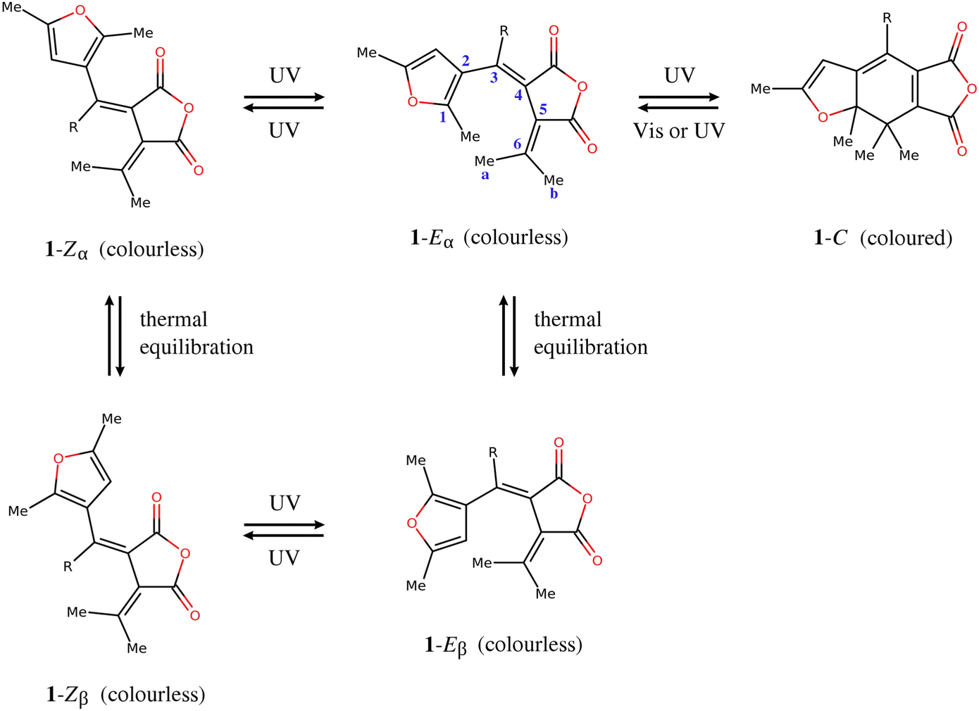 | ||
| Fig. 1 Molecular structures and photochemistry of furylfulgides in the series 1. Here, R denotes an alkyl substituent. | ||
Another isomer, the Eβ isomer, differs from the Eα isomer in the orientation of the furyl group. In the solution phase, the two isomers exist in equilibrium with one another.12 Unlike the Eα isomer, the Eβ isomer is incapable of photocyclisation, but it does undergo reversible photoisomerisation into the Zβ isomer. (The two Z isomers, Zα and Zβ, are in thermal equilibrium with one another.) From the standpoint of photochromism, the E ⇌ Z photoisomerisations of furylfulgides are undesirable side reactions. Recently, however, Filatov and coworkers13,14 have proposed that they can potentially serve as the basis for a new class of light-driven molecular motors.
In order to provide context for the present study, which will focus on the excited-state relaxation dynamics of furylfulgides, we first provide an overview of relevant earlier work in this area. For a more comprehensive discussion of the structural design and photochemistry of furylfulgides and related compounds, the reader is referred to the review paper by Yokoyama15 and to the more recent one by Renth and coworkers.16
The relaxation dynamics of furylfulgides following photoexcitation has been the subject of several spectroscopic studies. Notably, Handschuh and coworkers17 studied the relaxation dynamics of the E isomers of Me-1 and another furylfulgide in the solution phase with the use of TA spectroscopy with subpicosecond time resolution. The TA spectrum was fitted with a kinetic model which included two reaction pathways for photocyclisation: a direct pathway, and an indirect pathway which leads through an intermediate species I.17 In this model, the Eα and Eβ isomers were not differentiated, and the E → Z photoisomerisation reactions were neglected.17 On the basis of the fit to the spectroscopic data, Handschuh et al. inferred that both the direct and the indirect pathways are involved in the reaction mechanism.17 In that model, the direct pathway was characterised by a time constant of roughly 3.3 ps, while the indirect pathway was slower because of trapping in the reaction intermediate I.17 This sequence of events is illustrated in Scheme 1.
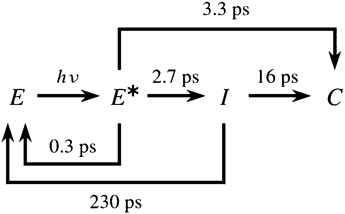 | ||
| Scheme 1 Kinetic model of the photorelaxation process of furylfulgide Me-1 proposed by Handschuh et al.17 | ||
In another study to investigate the photochemistry of the E isomers of compound Me-1 with the use of TA spectroscopy, Siewertsen et al.18 put forward a markedly different mechanism. These authors reported that the early stages of the relaxation dynamics involve two processes with time constants of 0.10 ps and 0.25 ps. The shorter time constant was assigned to the photocyclisation reaction of the Eα isomer, while the longer one was attributed to the E → Z photoisomerisation reactions of the Eα and/or the Eβ isomers.18 In this regard, Siewertsen et al. noted that they were unable to determine whether the Z photoproducts originate mainly from the Eα isomer, or from the Eβ isomer.18 Both these possibilities are illustrated in Scheme 2. Vibrational cooling of the photoproducts was reported to take place over a period of roughly 10 ps.18 In contrast to the earlier study by Handschuh et al.,17 Siewertsen and coworkers found no evidence for an additional, slower, photocyclisation pathway, or for the involvement of a long-lived intermediate.
 | ||
| Scheme 2 Two kinetic models for the photorelaxation process of Me-1 considered by Siewertsen et al.18 | ||
Moreover, Siewertsen et al. performed electronic structure simulations in which the ground- and excited-state potential energy surfaces (PESs) of Me-1 were scanned along the C1–C6 distance, and along the C2–C3 = C4–C5 torsion angle.18 For the description of electronic structures, these authors employed density functional theory (DFT) for the singlet ground state (S0), and time-dependent DFT (TDDFT) for the lowest singlet excited state (S1). Basing on these calculations, it was concluded that the photocyclisation reaction of the Eα isomer and photoinduced ring opening both begin in the S1 state, and are mediated by a conical intersection (CI) with the S0 state that is located at a C1–C6 distance of roughly 2.3 Å.
A subsequent study by the same group addressed the photoinduced ring-opening reactions of compounds Me-1, i-Pr-1 (the compound in the Series 1 with an isopropyl group), and two other more extensively modified furylfulgides.19
Further insight into the mechanism of furylfulgide photocyclisation and photoinduced ring opening was provided by the theoretical study by Tomasello and coworkers.20 In that study, the electronic structure of the system was treated with the CASPT2//CASSCF approach – second-order complete active space perturbation theory21 (CASPT2) single-point energies at molecular geometries optimised at the complete active space self-consistent field22 (CASSCF) level of theory. Using this advanced methodology, Tomasello et al. mapped out the full reaction pathway for photocyclisation and photoinduced ring opening. As shown schematically in Fig. 2(a), the photocyclisation reaction is triggered by excitation of the Eα isomer into the zwitterionic S1 state.20 Following the initial photoexcitation, the molecule is driven by the slope of the PES of the S1 state towards the S1/S0 CI seam.20 In the vicinity of the S1/S0 CI seam, the molecule undergoes internal conversion to the S0 state. Once in the S0 state, the reaction path bifurcates: part of the nuclear wavepacket relaxes towards the closed-ring isomer, while the remainder is reflected back towards the open-ring isomer.20
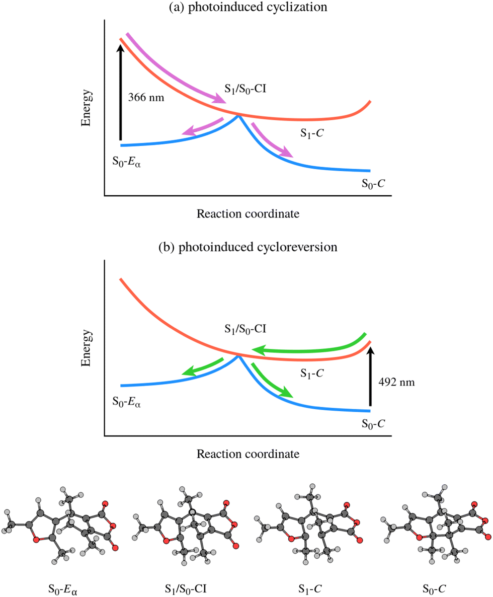 | ||
| Fig. 2 Overview of the mechanisms of (a) photocyclisation and (b) photoinduced ring opening of Me-1 and related furylfulgides as reported in the study by Tomasello and coworkers.20 The reaction coordinate, viewed from left to right, corresponds to ring closing. The key molecular structures along the reaction coordinate are depicted on the bottom. | ||
Regarding, in turn, the photoinduced ring opening reaction, Tomasello et al. predicted that it is mediated by the same S1/S0 CI seam as the photocyclisation reaction20 (see Fig. 2(b)). This is in agreement with the hypothesis put forward by Siewertsen et al.18
As for other studies, Schönborn and coworkers performed nonadiabatic molecular dynamics (NAMD) simulations of the photorelaxation processes of the Eα and Eβ isomers of furylfulgides i-Pr-123 and, in a later study, Me-1.24 In these simulations, the electronic structure of the system was treated with the semiempirical orthogonalisation-corrected method OM325–27 in a multireference configuration interaction (MRCI) framework.28 Furthermore, the CASPT2//CASSCF combination of methods was used in a supporting role, for the characterisation of minimum-energy geometries along S1/S0 CI seams (S1/S0 MECIs). These static calculations revealed that Me-1 and i-Pr-1 each possess three minimum-energy geometries (MECIs) along the S1/S0 CI seam, of which the first lies along the reaction coordinate for photocyclisation, and the other two are ethylenic-type MECIs which arise from twisting around the C3C4 and the C5C6 double bonds.23,24 The NAMD simulations, in turn, showed that internal conversion from the S1 state into the S0 state does not only take place in the immediate vicinity of the MECI structures, but rather, it occurs along an extended segment of the S1/S0 CI seam.23,24 In the case of the Eα isomer of furylfulgide Me-1, the predominant pathway involved nonradiative deactivation near the ethylenic MECI associated with twisting around the C3C4 bond, accounting for 80% of the total number of simulated trajectories for the Eα isomer.24 Roughly half of those simulated trajectories which approached that MECI went on to complete a full rotation around the C3C4 bond, giving a Eα → Z photoisomerisation quantum yield (QY) of 0.43.24 Photocyclisation (Eα → C), in turn, was less efficient, with a QY of only 0.04.24 As the authors were careful to point out, the NAMD simulations overestimated the overall QY of E → Z photoisomerisation (i.e. for an equilibrium mixture of the Eα and the Eβ isomers) relative to experiment, while underestimating the QY of photocyclisation (Eα → C).
Furthermore, Schönborn et al. found that on going from furylfulgide Me-1 to i-Pr-1, the QY of E → Z photoisomerisation decreased markedly, while the QY of photocyclisation increased.23,24 The direction of these changes was noted to be consistent with experimental data.23,24 From the results of the NAMD simulations, Schönborn et al. concluded that a bulky alkyl substituent at carbon atom C3 has a twofold influence on the photochemistry of furylfulgides: it causes the molecule to adopt a ground-state geometry which promotes photocyclisation (pre-orientation), and, furthermore, following photoexcitation, it drives the molecule towards the region of the S1/S0 CI seam which mediates photocyclisation.23,24
The studies reviewed above leave open the question of the relative importance of the various relaxation pathways of the Eα and Eβ isomers of furylfulgides. This problem is difficult to address with experimental methods alone, as the Eα and Eβ isomers exist in thermal equilibrium with one another, and their photoabsorption spectra overlap, meaning that they cannot be photoexcited selectively. In principle, computer simulations are well positioned to resolve the question of the relative contributions of the various relaxation processes, because the individual isomers can be modelled in isolation from one another. In this regard, if the results of the NAMD simulations by Schönborn et al.23,24 are taken at face value, then the most important side reactions are photoisomerisations around the C3C4 and C5C6 double bonds. However, these authors have noted that, in the case of furylfulgide Me-1, the NAMD simulations significantly overestimated the overall QY of E → Z photoisomerisation. Hence, there is a need for a re-examination of the roles of the different relaxation pathways in the overall mechanism.
In order to clarify the quantitative picture of the photorelaxation of furylfulgides, in the present study we performed NAMD simulations of the excited-state dynamics of the Eα and Eβ isomers of Me-1 as a representative member of this important class of photochromic compounds. In our simulations, the electronic structure of the molecule was treated with the use of spin-flip TDDFT29,30 (SF-TDDFT), a variant of the TDDFT method where the states of interest are obtained through spin-flipping excitations from a high-spin triplet reference determinant. Crucially, benchmarking against extended multi-state multireference second-order perturbation theory31 (XMS-CASPT2) indicates that SF-TDDFT achieves excellent accuracy for the relevant ground- and excited-state PESs of furylfulgides in the series 1. The emergent reaction pathways were identified automatically by employing k-means clustering (KMC),32,33 a pattern recognition algorithm which partitions observations (in this case, molecular geometries) into clusters whose elements are similar to each other, and different from those in other clusters. The application of the KMC algorithm affords an unprecedented level of insight into the dynamics of the photoexcited molecule, allowing a detailed comparison to spectroscopic data and the experimentally-determined photoproduct distribution.
The rest of this paper is organised as follows. We first discuss the setup of the NAMD simulations, and the pattern recognition procedure that was employed in order to analyse the results. We then examine the relaxation processes of the Eα and Eβ isomers of furylfulgide Me-1 in separation from one another. Finally, we use the simulation results as a basis to construct a model of the photochemistry of a sample containing both isomers at equilibrium, and tie it in with the available experimental data.
2 Computational methods
2.1 NAMD simulations
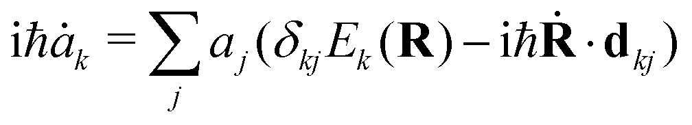
The aim of our NAMD simulations was to characterise the relaxation processes of the Eα and Eβ isomers of furylfulgide Me-1 following photoexcitation into the S1 state. The simulation model consisted of a single isolated molecule of the given isomer, and its electronic structure was treated with SF-TDDFT. The time evolution of the molecule was propagated with the fewest switches surface hopping34–36 (FSSH) method. In this approach, the nuclear wavepacket of the system is represented by an ensemble of mutually independent semiclassical trajectories. In each simulated trajectory, nuclear dynamics is described by means of classical mechanics, while the electronic structure of the molecule is treated quantum mechanically. The overall wave function Ψ(r,t;R) of the electrons along a given nuclear trajectory R = R(t) is expressed as a linear combination of adiabatic electronic states {ψj(r;R)} with time-dependent coefficients {aj(t)}: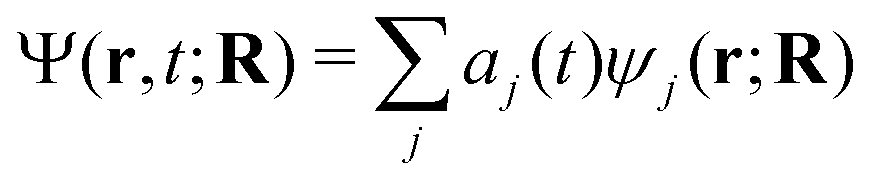 | (1) |
 | (2) |
| dkj = 〈ψk(r;R)|∇R|ψj(r;R)〉 | (3) |
 | (4) |
The NAMD simulations were performed with our existing “wrapper” program,37 which features an interface to the electronic structure program Q-Chem.38,39 For a detailed description of our implementation, the Reader is referred to ref. 37 The dynamics of the nuclei (eqn (4)) was propagated with the use of the velocity Verlet integrator with a time step of 0.5 fs. The expansion coefficients {aj(t)} were corrected for decoherence using the technique proposed by Granucci and Persico.40 As recommended in ref. 40, the value of the damping constant for the correction was set to C = 0.1Eh (Hartree).
The electronic structure of the molecule during the simulated dynamics was monitored by following the classical populations of the S0 and S1 states. As per the usual convention, the classical population (Pj) of the j-th adiabatic state from among those included in the linear expansion 1 is defined as the fraction of trajectories that is currently evolving in that state:
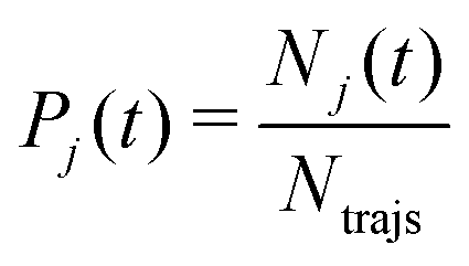 | (5) |
The initial conditions for the NAMD simulations were generated as follows: the ground-state equilibrium geometries of the Eα and Eβ isomers of Me-1 were optimised at the DFT level of theory. Afterwards, the normal modes of either isomer were calculated numerically using analytical gradients. The initial conditions (sets of nuclear positions and velocities) were sampled from the Wigner distribution of either isomer in its vibrational ground state. As discussed in ref. 41 and 42, molecular dynamics simulations of molecules containing hydrogen atoms are prone to an artificial leakage of zero-point energy from the stretching modes of hydrogen-heavy atom bonds to other vibrational modes. In order to mitigate this problem, when generating the Wigner distribution we froze the highest sixteen vibrational modes, which correspond to C–H stretching modes. At the outset of each trajectory, the S1 state was chosen the current state, and its expansion coefficient was set to unity. Ntrajs(Eα) = 75 trajectories were generated for the Eα isomer, and Ntrajs(Eβ) = 50 for the Eβ isomer. For either isomer, the trajectories were propagated for a period of 500 fs. We did not experience any crashes, or convergence failures, in the SF-TDDFT calculations, and all trajectories that were propagated for either isomer completed successfully.
2.2 Electronic structure calculations
The DFT and SF-TDDFT calculations were performed with the computational chemistry software package Q-Chem,38,39 version 5.1.2. The SF-TDDFT calculations were performed in the collinear approximation, and furthermore, the Tamm-Dancoff approximation43 was imposed. We employed the 50–50 exchange-correlation functional29 (50% Hartree-Fock + 8% Slater + 42% Becke for exchange, and 19% VWN + 81% LYP for correlation), which is based on the well-known B3LYP functional,44,45 but includes a larger fraction of Hartree-Fock exchange. For the sake of computational efficiency, which is of utmost importance in molecular dynamics simulations, we used the relatively small 6-31G(d) basis set.46,47 The nonadiabatic coupling vector (NACV) between the S0 and S1 states was calculated analytically via the method of Zhang and Herbert.48 Because the calculation of the NACV is expensive in terms of computing time, during the NAMD simulations we began calculating the NACV only after the energy gap between the S0 and S1 states in a given trajectory decreased to below a threshold of 0.5 eV for the first time. Once that had happened, the NACV was subsequently calculated for the remainder of the given trajectory, even if the energy gap increased to over 0.5 eV again.With these settings, propagating a single 500 fs-long trajectory requires 1000 gradient evaluations, and an average of around 650 NACV evaluations. (The exact number of NACV calculations along the given trajectory depends on when the S1–S0 energy gap decreases to below 0.5 eV.) The cost of a gradient calculation and a NACV calculation is about the same, at roughly 75 CPU minutes on an Intel(R) Xeon(R) E5-2670 2.3 GHz processor. Thus, propagating a single trajectory takes roughly 2000 CPU hours. In our study, we have propagated a total of 125 simulated trajectories (75 and 50, respectively, for the Eα and the Eβ isomers), and the total cost of our simulations amounted to some 250![[thin space (1/6-em)]](https://www.rsc.org/images/entities/char_2009.gif) 000 CPU hours.
000 CPU hours.
In closing this section, we acknowledge that although there has been progress in evaluating the performance of SF-TDDFT in various contexts,49–55 it still remains a relatively untested method. In order to verify whether SF-TDDFT is reliable for the topographies of the ground- and excited-state PESs of compound Me-1, we have compared its predictions to the benchmark provided by the XMS-CASPT2 method, which is the highest-level electronic structure method that we are able to apply to furylfulgides. The details of these benchmark calculations are given in Section S1 of the ESI.† Encouragingly, we found that the two methods are in very close agreement for the PESs of the S0 and S1 states. We therefore believe that our NAMD simulations are realistic not only in the qualitative sense, but they can also serve as a basis for the estimation of quantities such as photoisomerisation QYs and relaxation time scales.
2.3 Pattern recognition analysis
In the electronic ground state, the open-ring form of furylfulgide Me-1 exhibits rotamerism around the C2–C3 bond, but otherwise the molecule is fairly rigid. Once photoexcited into the S1 state, however, it becomes much more flexible: given a suitable orientation of the furyl grop, it can undergo cyclisation, but alternatively it can also undergo photoisomerisation around the C3C4 or the C5C6 bonds. What is more, in the course of our NAMD simulations, it became evident that the anhydride ring is flexible enough to permit a partial rotation around the C4–C5 bond. In hindsight, the flexibility of the anhydride ring is unsurprising – all five bonds comprising that ring are formally single bonds.
The flexibility of the photoexcited molecule means that the relaxation dynamics is a multidimensional process: in order to obtain a comprehensive picture of the time evolution of molecular geometry in the simulated trajectories, one needs to take into account several structural parameters (or, internal coordinates). The exact choice of parameters is, to some extent, arbitary, as long as it provides a good description of molecular geometry. Presently, we elected to monitor the C1⋯C6 distance (denoted R16), which describes cyclisation, and the following four torsion angles: C1C2–C3C4 (τ1234), C2–C3C4–C5 (τ2345), C3C4–C5C6 (τ3456), and C4–C5C6Ca (τ456a).
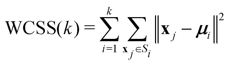
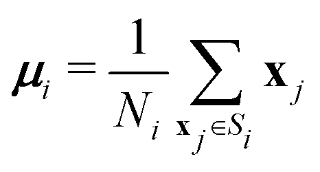
The fairly high dimensionality of the data poses a challenge for interpretation, as it is far from obvious how to make out distinct reaction pathways (subsets of mutually similar trajectories), or even how many reaction pathways there are. In order to facilitate the analysis of the simulation results, we employed the KMC algorithm,33 a well-known and widely used pattern recognition method. KMC takes as input a number (n) of observations ({x1, x2,…, xn}), where each observation is a d-dimensional real vector. The components of this vector are the input variables, which in this context are called features. The algorithm partitions the observations into a predefined number (k) of clusters ({S1, S2,…, Sk}), in such a way that each observation is assigned to the cluster with the nearest centroid (or, geometric center). The optimal partitioning for the given value of k is found by minimising the within-cluster sum of squares (WCSS):
 | (6) |
 | (7) |
In the present case, the observations consist of a set of “snapshots” from the NAMD simulations, which is to say, a set of molecular geometries at a time point t. This situation is depicted schematically in Fig. 3. Our goal is to partition the snapshots into k clusters in such a way that each cluster contains geometries which are similar to each other, and different from those in other clusters. Note that we are not partitioning the entire ensemble of simulated trajectories, but rather, a set of snapshots at a time point t during the simulations. Furthermore, we consider the sets of trajectories starting from the Eα isomer and from the Eβ isomer separately.
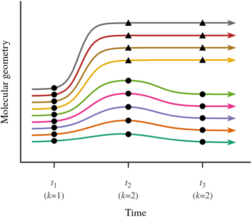 | ||
| Fig. 3 Schematic illustration of the analysis of an ensemble of simulated trajectories with the use of the KMC algorithm. The colored lines represent the individual trajectories. In this example, the ensemble of trajectories bifurcates into two relaxation pathways. The partitioning of snapshots from different time points during the simulation into clusters is indicated with circles and triangles. At time t1, the simulated trajectories are best described as forming a single cluster, whereas at times t2 and t3, the snapshots are partitioned into two clusters. | ||
The right value for k, which is the number of distinct relaxation pathways, is not known a priori, but the principle of parsimony (Occam's razor) dictates that we choose the lowest possible k that gives a satisfactorily low WCSS. This reasoning leads to the so-called elbow method56,57 for choosing the right value for k: the lowest value is chosen that converges, or nearly converges, the WCSS. This is the approach that we adopted in our analysis. We note here that the right value for k can and does change with time. This is because, for either isomer of compound Me-1, all simulated trajectories start out narrowly distributed in the Franck-Condon region. Only later do the simulated trajectories spread out in the configuration space, and fork out into distinct relaxation pathways.
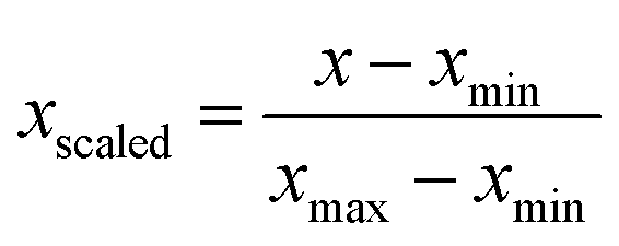
One final issue which needs to be discussed is the way the molecular geometry is represented for analysis with the KMC algorithm. KMC requires that all features vary on a similar scale, and are measured in the same units or are dimensionless. The set of five internal coordinates defined above does not meet this condition, as one of the five is an interatomic distance, while the other four are torsion angles. Another complication is that a torsion angle has a periodic discontinuity at a value of ±180°. We addressed this latter issue by taking the cosines of the four torsion angles instead of the torsion angles themselves. Unlike the torsion angles themselves, their cosines are continuous functions of molecular geometry. The final list of features which are passed on to the KMC algorithm is therefore as follows: R16, cos(τ1234), cos(τ2345), cos(τ3456), and cos(τ456a).
Prior to analysis, all five features were scaled with the standard min-max scaler, which shifts the data in such a way that all features lie in the range [0,1]:
 | (8) |
We used the implementation of the KMC algorithm in the scikit-learn library,58 version 0.24.2, with Python 3, version 3.6.9. As per the default settings, the assignment of observations to clusters was performed using Lloyd's algorithm.33 The solution obtained with this algorithm is dependent on the initial conditions. For this reason, when running the algorithm, we always started from 25 random choices of initial conditions, and selected the best result, namely, the one that gives the lowest WCSS.
2.4 Calculation of quantum yields
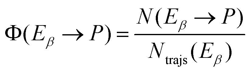
A key point of comparison between our NAMD simulations and experimental data is the photoproduct distribution resulting from the irradiation of an equilibrium mixture of the Eα and Eβ isomers of Me-1. In the present section, we outline the calculation of the QYs of the various photochemical reactions which occur in this system.Let us begin with the photoproduct distributions of the relaxation processes of the Eα and Eβ isomers individually. We assume that the photoisomerisation reactions of either isomer are complete by the time that the NAMD simulations were terminated (t = 500 fs). This is justified by the fact that, by this time, both isomers have almost fully undergone internal conversion into the vibrationally hot ground state, and they are unlikely to undergo further isomerisations, other than α ⇌ β rotamerism. With this assumption, the photoproduct distribution for either isomer may be equated with the final cluster assignment. Thus, for a given photoproduct P, the QYs of the processes Eα → P and Eβ → P (denoted Φ (Eα → P) and Φ (Eβ → P)) are calculated as follows:
 | (9) |
 | (10) |
For the purposes of the analysis of QYs, the photoproduct Zα and Zβ isomers are considered together, as are the unreacted Eα and Eβ isomers. This is because all open-ring isomers undergo α ⇌ β rotamerisation and, within a short time of the irradiation of the sample, they will re-establish the Zα ⇌ Zβ and the Eα ⇌ Eβ equilibria.
Because the QYs of the Eα → P and the Eβ → P processes are each calculated on the basis of a finite number of simulated trajectories, they are subject to statistical uncertainties associated with finite sample sizes. The treatment of the statistical uncertainties in the calculated QYs is discussed in more depth in Section S4 of the ESI.†
In the solution phase, the Eα and Eβ isomers coexist in equilibrium with one another. We denote their mole fractions as x(Eα) and x(Eβ), respectively. Prior to the irradiation of the sample, no other isomer is present, so that x(Eα) + x(Eβ) = 1. Suppose now that the sample is irradiated with monochromatic radiation which falls within the first photoabsorption band of the E isomer mixture (ca. 325–375 nm). The overall QY of photoproduct P (denoted ΦOA(P)) is estimated as the sum of the QYs for the Eα → P and Eβ → P processes weighted by the mole fractions of the respective starting isomers:
| ΦOA(P) = x(Eα)Φ(Eα → P) + x(Eβ)Φ(Eβ → P) | (11) |
As with the QYs of the Eα → P and Eβ → P processes, the overall QY is subject to statistical uncertainty. A separate issue is that the exact population ratio of the Eα and Eβ isomers is unknown. To the best of our knowledge, the population ratio has not been determined experimentally; in some previous studies, it was estimated by means of semiempirical59 and DFT18 calculations. In view of the importance of the population ratio for the calculation of the photoproduct distribution, in the present study we sought to obtain an improved estimate. To this end, we carried out a series of DFT thermochemistry calculations with several choices of exchange–correlation functional. Moreover, in one set of calculations, single-point energy corrections were evaluated with the domain-based local pair natural orbital coupled cluster with perturbative triples60,61 (DLPNO-CCSD(T)) method at molecular geometries optimised at the DFT level. The details of these calculations are given in Section S3 of the ESI.† Our best estimate is that the mole fraction of the Eα isomer lies in the range of 0.8 ± 0.1, where the width of this interval reflects the spread in the predictions of the various DFT functionals and the DLPNO-CCSD(T) method. The uncertainty in the mole fractions of the two isomers contributes to the uncertainty in the calculated overall QYs.
3 Results and discussion
3.1 Relaxation dynamics of the Eα isomer
Fig. 4 provides an overview of the dynamics of the Eα isomer photoexcited initially into the S1 state. Accompanying this data, as part of the ESI,† we provide animations of eight representative simulated trajectories. Each animation shows the time-evolution of the molecular geometry and the energies and populations of the S0 and S1 states. The passage of time is indicated with a vertical black line moving along the time axis. The currently occupied state is marked with a black circle. The initial photoexcitation occurs at t = 0 fs.
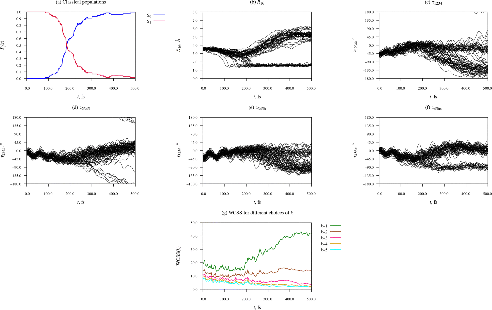 | ||
| Fig. 4 Time-evolution of electronic structure and molecular geometry during the relaxation dynamics of the Eα rotamer of furylfulgide Me-1. | ||
Panel (a) of Fig. 4 shows the classical populations of the S0 and S1 states in the ensemble of simulated trajectories. The stepped appearance of the plot is a consequence of the fact that when trajectories hop from one state to another, the classical populations change discontinuously. At the outset of the simulations, all trajectories were occupying the S1 state, such that its population was equal to 1. From around 100 fs after the initial photoexcitation, the simulated trajectories began encountering the CI seam between the S1 and S0 states, and hopping down from the S1 state into the S0 state. The onset of internal conversion into the S0 state manifests itself as a sharp drop in the classical population of the S1 state, and a corresponding increase in the classical population of the S0 state. From around t = 300 fs until the end of the simulations at t = 500 fs, only a few simulated trajectories remained in the S1 state. The median earliest hopping time was calculated to be 184 fs.
Panels (b) to (f) of Fig. 4 characterise the time-evolution of molecular geometry by showing the distance R16 and values of the torsion angles τ1234, τ2345, τ3456, and τ456a among the ensemble of simulated trajectories. Although the relaxation dynamics and the resulting dataset are quite complex, some trends in the data are readily apparent. At the time of the initial photoexcitation (t = 0), the simulated trajectories were distributed in the Franck-Condon region, the narrow region of the configuration space near the ground-state equilibrium geometry of the Eα isomer. During the initial 100 fs-long period after the initial photoexcitation, the trajectories remained narrowly distributed. In fact, it can be seen that the vibrational modes of the molecule which modulate the torsion angles τ2345, τ3456, and τ456a maintained some degree of phase coherence for roughly 100–150 fs after the photoexcitation.
Between around t = 100 fs and t = 300 fs, the ensemble of simulated trajectories branched out into multiple (at least two, possibly more) relaxation pathways. The exact number of distinct relaxation pathways will be determined later on with the use of the KMC algorithm. As expected, in a number of trajectories, 20 to be specific, the molecule underwent cyclisation. The ring closing is clearly visible in Fig. 4(b), which shows values of the C1⋯C6 distance – in 20 of the simulated trajectories, R16 contracted to around 1.6 Å, which is typical of sterically strained carbon–carbon single bonds. In these 20 trajectories, R16 subsequently oscillated in the range of roughly 1.4 Å to 1.8 Å, which shows that the newly formed C1–C6 bond remained intact for the duration of the simulation. Furthermore, in these 20 trajectories, the dimethylmethylene group containing atom C6 (the = C6Me2 group) rotated by roughly 90° around axis of the C5C6 bond, permitting the formation of the C5–C6 bond. The rotation around the C5C6 bond is clearly visible in Fig. 4(f), which shows values of the C4–C5C6–Ca torsion angle (τ456a).
Moreover, inspection of Fig. 4(d), which shows values of the C2–C3C4–C5 torsion angle (τ2345), reveals that in 7 of the simulated trajectories, the molecule underwent a substantial rotation around the C3C4 bond, which is to say, Eα → Zα photoisomerisation. In Fig. 4(d), these trajectories can be seen splitting off from the remainder of simulated trajectories, and shifting towards lower values of τ2345. 6 of these trajectories crossed the ±180° line, while the seventh was lagging behind the other two, and it did not reach the ±180° line by the time the simulations were discontinued at t = 500 fs. All 7 of these trajectories hopped down from the S1 into the S0 state in the vicinity of the S1/S0 CI seam at τ2345 ≈ 90°.
At early times during the simulations, up to around t = 100 fs, there is a slight reduction in WCSS on going from k = 1 to k = 2, but increasing k beyond 2 does not bring about a significant further lowering of WCSS. From our earlier discussion, we know that at this stage, the distribution of simulated trajectories was fairly compact. This indicates the KMC algorithm is simply picking up on relatively minor differences between the molecular geometry in different simulated trajectories, and there is not yet any indication that the ensemble of trajectories has split into distinct relaxation pathways.
During the time interval from around t = 100 fs to around t = 200 fs, the k = 1, k = 2, and k = 3 curves separate out, and they remain separated for the remainder of the simulation time of 500 fs. This is a clear-cut signature of the ensemble of simulated trajectories branching out into a number of relaxation pathways. Meanwhile, the k = 4 and k = 5 curves always remain just below the k = 3 curve. The fact that the k = 3 curve is well separated from the k = 2 curve, while in turn the k = 4 and k = 5 curves are close to the k = 3 curve, indicates that the underlying data at t > 200 fs is well described by a partitioning into three clusters.
Having thus determined that the ensemble of simulated trajectories split into three relaxation pathways, we can now examine these pathways in more detail. Fig. 5 shows how the KMC algorithm partitions the molecular geometries at three time points during the NAMD simulations: t = 0 fs, 250 fs, and 500 fs. Basing on what was said above, at t = 0 fs we interpret all snapshots from the NAMD simulations as comprising a single cluster (k = 1), whereas at t = 250 fs and at t = 500 fs, we have set k = 3.
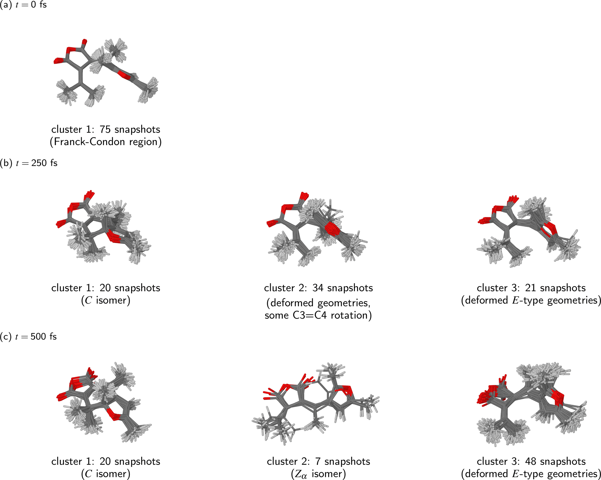 | ||
| Fig. 5 Clustering of snapshots at different time points during the NAMD simulations of the photorelaxation process of the Eα isomer. We assume k = 1 cluster at t = 0 fs, and k = 3 clusters at t = 250 fs and at t = 500 fs. The clusters were visualised by overlaying all molecular geometries comprising the given cluster. | ||
It can be seen that at the time of the initial photoexcitation (t = 0 fs), the molecular geometries were indeed localised in a narrow region of configuration space around the ground-state equilibrium geometry – the Franck-Condon region. This is a consequence of the fact that the initial conditions for the NAMD simulations were generated by sampling from the Wigner distribution of the molecule in the vibrational ground state.
By t = 250 fs, the simulated trajectories had spread out in the configuration space. Of the three clusters into which the snapshots have been partitioned, the first consists of 20 snapshots, and it clearly represents the closed-ring photoproduct (isomer C). On the other hand, the second and third clusters (containing 34 and 21 snapshots, respectively) correspond to deformed open-ring geometries. A shared characteristic of the geometries comprising the second cluster appears to be twisting around the C3C4 bond. However, none of the molecular geometries comprising the second cluster has yet completed a full isomerisation around the C3C4 bond. As regards the third cluster, its defining characteristic appears to be intramolecular rotation around the C2–C3 bond. The second and third clusters actually appear somewhat similar to one another. It seems that, at this stage during the relaxation process, only the closed-ring isomer had emerged as a distinct photoproduct, and the remaining molecular geometries were still rather undifferentiated.
Finally, by the time the simulations were concluded (t = 500 fs), all three clusters identified by the KMC algorithm correspond to recognizable photoproducts. The contents of the first cluster (20 snapshots) is the same as at t = 250 fs: it contains snapshots from those trajectories in which the molecule has undergone photocyclisation. On the other hand, the compositions and sizes of the second and third clusters have changed considerably. At t = 500 fs, the second cluster contains only 7 snapshots, all of which adopt the Zα isomeric form. The inspection of their geometries shows that the photoisomerisation takes place through a one-bond-flip mechanism – that is to say, the C3C4 bond is the only one to undergo a rotation by roughly 180°. The adjacent C2–C3 bond does not go through a significant rotation.
The third and largest cluster (48 snapshots) comprises unreacted molecular geometries, which is to say, those where the molecule has undergone neither photocyclisation nor double-bond photoisomerisation. All of these molecular geometries show a partway rotation around the C2–C3 bond, and also a conspicuous deformation of the anhydride ring. These structural changes presumably occurred because in most of the trajectories from which these snapshots originate, the hopping from the S1 state into the S0 state took place in a region of the configuration space where the PES of the S0 state is strongly repulsive with respect to the distance between atoms C1 and C6. As a result, the furyl group and the dimethylmethylene group containing atom C6 were pushed away from one another. Possibly, this effect ultimately leads to a full rotation around the C2–C3 bond, and the formation of the Eβ isomer, although the simulation time of 500 fs was too short for that to happen.
In order to shed more light on the role of the torsional degrees of freedom (rotation around the C2–C3 and the C3C4 bonds), we scanned the PES of the S1 state as a function of the torsion angles τ1234 and τ2345. The detailed description of this calculation is given in Section S2 of the ESI.† The results indicate that rotation around the C3C4 bond (E → Z photoisomerisation) is driven by the topography of the PES of the S1 state. Conversely, the topography of the S1 state does not appear to provide a driving force for rotation around the C2–C3 bond. We hypothesize that when a rotation around the C2–C3 bond does happen, it is caused by a redistribution of vibrational energy from other modes.
As explained in Section 2.4, the final cluster assignment serves as the basis for the estimation of the photoproduct distributions. The calculated QYs for the pure Eα isomer are shown as the first entry in Fig. 8. The QY of Eα → C photocyclisation is 0.27 ± ± 0.10, and that of Eα → Z photoisomerisation is 0.09 ± 0.07. The remaining fraction of photoexcited molecules (0.64 ± 0.11) deactivate to the ground state in a deformed E-like geometry; we denote this outcome Eα → E. It is tempting to think of this latter relaxation pathway as a strictly negative phenomenon, but it does ultimately regenerate the photochromically active Eα isomer. In this sense, it contributes to the photostability of the Eα isomer.
The relatively low incidence of Eα → Z photoisomerisation in our simulations requires some comment. As discussed in more detail in Section S1 of the ESI,† SF-TDDFT achieves excellent agreement with the benchmark provided by XMS-CASPT2. Moreover, during the NAMD simulations, we have propagated a relatively large number of trajectories, leading to a thorough sampling of the photoproduct distribution. For these reasons, we have confidence in the prediction that, Eα → Z photoisomerisation is only a minor relaxation pathway. At the same time, however, the photoproduct distribution predicted by our simulations stands in contrast to the results of the earlier theoretical study of Schönborn and coworkers,24 where Eα → Z photoisomerisation was found to be the predominant relaxation pathway of the Eα isomer of furylfulgide Me-1. In the work just cited, it was acknowledged that the overall QY of E → Z photoisomerisation was overestimated with respect to experiment, and this error was attributed to the neglect of solvent effects, and to other approximations inherent in the simulation model.24 However, the solvent is also absent in our own simulations, so the neglect of solvent effects is unlikely to be responsible. The most important difference between the simulation setup used by Schönborn et al.24 and in the present study is the choice of electronic structure method: in ref. 24, the ground- and excited-state PESs of the molecule were generated with the use of the semiempirical OM3/MRCI approach, whereas in the present study, the SF-TDDFT method is used. We therefore conjecture that the overestimation of the incidence of E → Z photoisomerisation in ref. 24 may reflect a systematic error in the PESs calculated at the OM3/MRCI level, which introduces a bias for E → Z photoisomerisation over photocyclisation.
3.2 Relaxation dynamics of the Eβ isomer
 | ||
| Fig. 6 Time-evolution of electronic structure and molecular geometry during the relaxation dynamics of the Eβ rotamer of furylfulgide Me-1. | ||
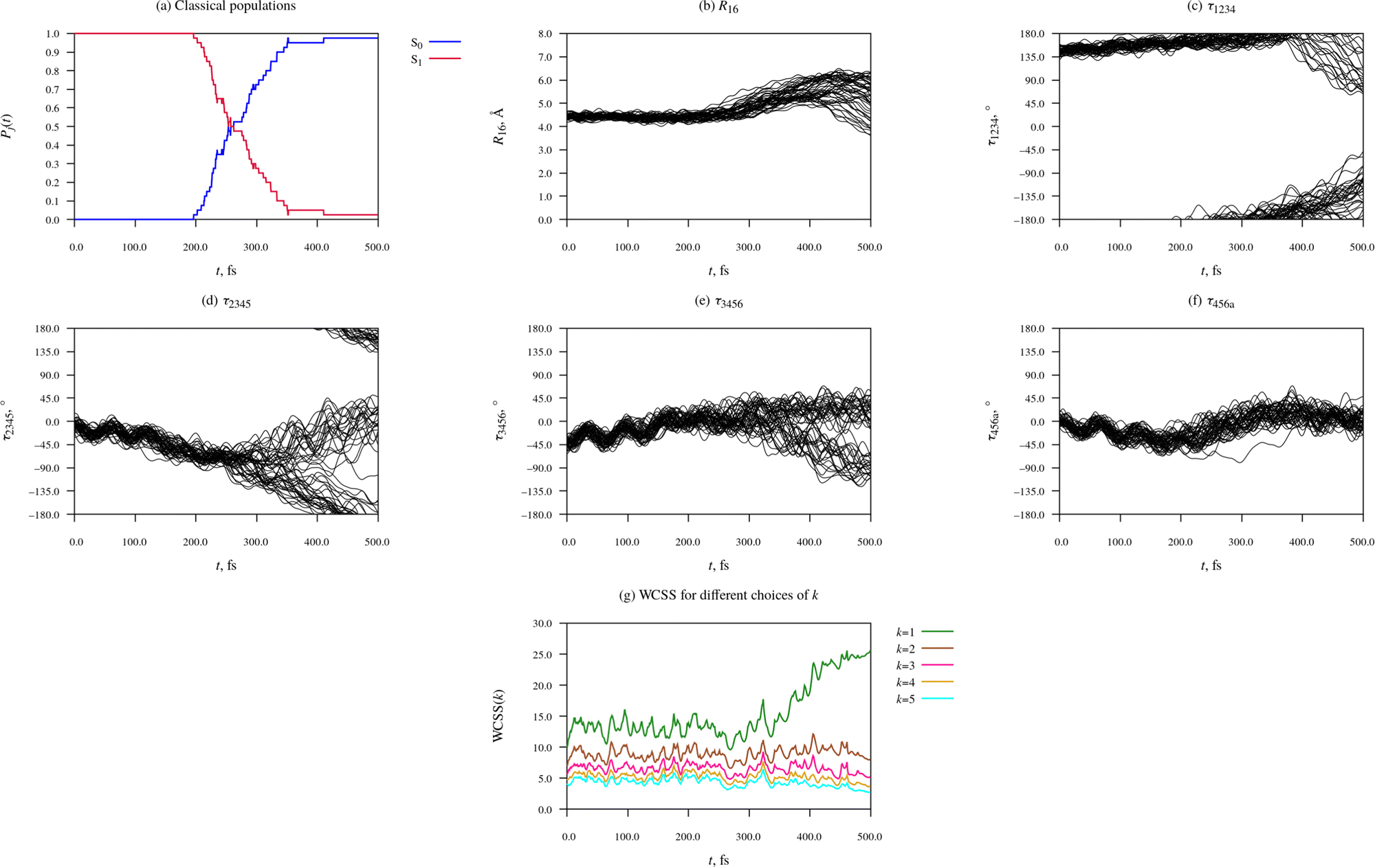
The first thing to note about the photorelaxation dynamics of the Eβ isomer is that internal conversion from the S1 state into the S0 state was somewhat slower than for the Eα isomer – whereas for the Eα isomer, the median earliest hopping time was 184 fs, for the Eβ isomer it was 254 fs.
Moreover, it is immediately apparent that the Eβ isomer did not undergo photocyclisation, as the C1⋯C6 distance (R16) did not decrease below 3 Å in any of the simulated trajectories. Instead, the relaxation dynamics of the Eβ isomer was dominated by torsional deformations of the heavy-atom skeleton. Shortly after the initial photoexcitation, the molecule began to undergo intramolecular rotations around the C3C4 bond and, to a lesser degree, also around the C2–C3, the C4–C5, and the C5C6 bonds. Until around t = 250 fs, the rotations in the different trajectories proceeded in a concerted fashion, such that the ensemble of trajectories as a whole remained fairly compact.
At around t = 300 fs, the ensemble of trajectories branched out into multiple (two or more) relaxation pathways. The forking into distinct pathways is clearly visible in the plots of the torsion angles τ1234, τ2345, and τ3456(Fig. 6(c)–(e), respectively), all of which began to spread out at around t = 300 fs. Roughly half of the simulated trajectories continued evolving in the negative τ2345 direction and eventually reach or approach the τ2345 = ±180°, which indicates that one of the emergent pathways is isomerisation around the C3C4 bond (i.e. Eβ → Z photoisomerisation). Most of the remaining trajectories were reflected back in the positive τ2345 direction, meaning that the other pathway can be described as failed Eβ → Z photoisomerisation.
At around t = 300 fs, the WCSS value for k = 1 begins to increase rapidly, while the WCSS values for k = 2 and for higher values of k remain stable, undergoing only minor fluctuations. The sharp rise of the k = 1 curve, together with the fact that the curves for k = 2 to 5 remain closely spaced, shows that the ensemble of simulated trajectories separated into exactly two relaxation pathways; there is no evidence for an additional third pathway.
The clusters identified by the KMC algorithm at different time points during the simulated dynamics (t = 0 fs, 250 fs, and 500 fs) are shown in Fig. 7. As stated above, from t = 0 fs until around t = 300 fs, the ensemble of simulated trajectories followed a single relaxation path. Indeed, it can be seen that at the t = 0 fs and t = 250 fs (Fig. 7(a) and (b), respectively), the molecular geometries were narrowly distributed in the configuration space of the system.
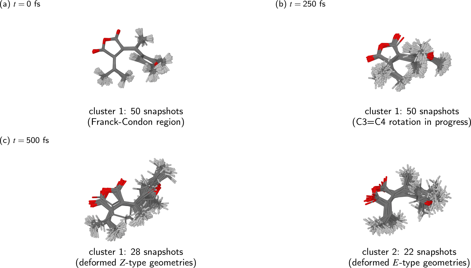 | ||
| Fig. 7 Clustering of snapshots at different time points during the NAMD simulations of the photorelaxation process of the Eβ isomer. We assume k = 1 cluster at t = 0 fs and at t = 250 fs, and k = 2 clusters at t = 500 fs. The clusters were visualised by overlaying all molecular geometries comprising the given cluster. | ||
By the end of the simulations at t = 500 fs, the ensemble of trajectories had branched out into two distinct relaxation pathways. Of the two clusters identified by the KMC algorithm at that point in time, the first consists of 28 snapshots, and corresponds to the photoproduct Z isomer. In most of these molecular geometries, the furyl group is oriented at roughly a right angle to the anhydride moiety, meaning that the photoproduct cannot be identified as either the Zα or Zβ isomer; it is best desribed as a vibrationally hot Z isomer whose molecular geometry is deformed away from the ground-state equilibrium geometry. The second cluster consists of the remaining 22 snapshots, all of which adopt a Eβ-type geometry. In many cases, the molecule displays a substantial deformation of the anhydride ring, and sometimes also a partial rotation of the furyl group around the C2–C3 bond.
The calculated QYs for the relaxation processes of the Eβ isomer are presented as the second entry in Fig. 8. The QY of Eβ → Z photoisomerisation is predicted to be 0.56 ± 0.14. The remaining fraction of photoexcited molecules (0.44 ± 0.14) deactivate to the ground state without undergoing photoisomerisation; we denote this outcome as Eβ → E.
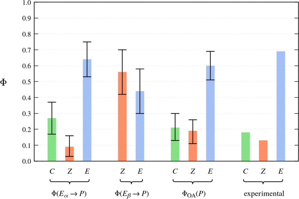 | ||
| Fig. 8 Photoproduct distributions (QYs) estimated on the basis of the NAMD simulations. For reference, the rightmost entry shows the experimentally-determined product distribution of Me-1 in toluene solution as reported in ref. 62. | ||
3.3 Overview of relaxation mechanism
The calculated photoproduct distribution of an equilibrium mixture of the Eα and Eβ isomers is presented visually as the third entry in Fig. 8. The calculated overall QYs (ΦOA(P)) are 0.21 ± 0.08 for photocyclisation (E → C), 0.19 ± 0.08 for E → Z photoisomerisation, and 0.60 ± 0.09 for no reaction (E → E). Rewardingly, the calculated photoproduct distribution coincides quite closely with the photoproduct distribution determined experimentally by Yokoyama and coworkers62 (the fourth entry in Fig. 8). In fact, the experimentally-determined QYs lie within the confidence intervals of the overall QYs estimated on the basis of the NAMD simulations. However, we place no special significance on this particular result. This is because the confidence intervals only account for statistical uncertainty and for the systematic uncertainty in the population ratio of the Eα and Eβ isomers. They do not account for other potentially significant sources of error, such as the neglect of solvent, and the approximations inherent in the FSSH method.
With the above caveat in mind, the good agreement with experiment means that our model of the photochemistry of furylfulgide Me-1 has passed a crucial test, as any major inconsistency between the simulation-based prediction of the photoproduct distribution and experimental data would indicate that the simulation model was inaccurate. According to our results, the closed-ring isomer (C) originates exclusively from the photocyclisation reaction of the Eα isomer. As for the Z isomers, these are formed in comparable proportions from the photoexcited Eα and Eβ isomers.
 | ||
| Scheme 3 Kinetic model of the relaxation dynamics of furylfulgide Me-1 based on the present simulations. | ||
A connection can be drawn to the findings of the joint spectroscopic and theoretical study by Siewertsen and coworkers.18 As mentioned in the Introduction section, these authors considered two possible mechanisms for the photochemistry of the E isomers of furylfulgide Me-1 in n-hexane solution. In the first mechanism (see Scheme 2a), the Eα isomer undergoes photocyclisation, and it is also responsible for the majority of the Z photoproducts. The second mechanism (Scheme 2b) instead envisions that it is mainly the minority Eβ isomer that gives rise to the Z photoproducts. The TA spectroscopic data was noted to be compatible with both these mechanisms. According to our simulations, the situation is somewhere in between these two limiting scenarios: both the Eα and Eβ isomers contribute to the formation of the Z photoproducts in similar amounts.
Siewertsen et al. further reported that the photorelaxation dynamics of the mixture of Eα and Eβ isomers is characterised by two time constants of 100 fs and 250 fs, of which the first attributed to cyclisation, and the second to E → Z isomerisations.18 Our NAMD simulations support the interpretation that cyclisation occurs on a slightly shorter time scale than E → Z isomerisations, but they do not reproduce the experimentally-observed time constants. More specifically, in the simulations, the onset of cyclisation occurs roughly at t = 100 fs, but most of those trajectories which undergo cyclisation do so at later times, at around t = 200 fs (see Fig. 4 in Section 3.1). Also, the E → Z photoisomerisations take roughly 500 fs to complete.
There is no grounds to believe that the NAMD simulations are artificially overestimating the amount of time required for the molecule to undergo either ring closing or E → Z photoisomerisation. As discussed in Section S1 of the ESI,† the SF-TDDFT method provides an accurate picture of the ground- and excited-state PESs along the reaction coordinate for both these processes. If anything, the neglect of solvent effects means that the simulations are likely to be underestimating the timescale of E → Z photoisomerisation.
In our assessment, the 100 fs time constant is too short to be assigned to a photocyclisation reaction, especially in a large molecule such as Me-1, where the ring closing involves the motion, relative to one another, of two fairly heavy chemical moieties. For this reason, and also due to the lack of agreement with the NAMD simulations, we hypothesise that the 100 fs time constant does not actually correspond to cyclisation, but can be instead attributed to an earlier event during the relaxation dynamics, presumably the initial motion of the nuclear wavepacket away from the Franck-Condon region. If this assignment is correct, it would follow that it is the longer time constant of 250 fs that corresponds to cyclisation. Leaving aside the question of the assignment of the rate constants, our simulations support the view that both photocyclisation and E → Z photoisomerisation take place within a few hundred femtoseconds of the initial photoexcitation.
On the other hand, the results of our simulations are incompatible with the kinetic model proposed by Handschuh and coworkers17 (see Scheme 1). The most serious discrepancy between that model and ours is the timescale of photocyclisation, which is several picoseconds in the model put forward by Handschuh et al.,17 but only a few hundred femtoseconds in our simulations. We believe that the disparity in timescale is too large to be attributed to the fact that the spectroscopic measurements by Handschuh et al.17 were performed in the solution phase, whereas our simulations do not include solvent effects. This is especially because the timescale of photocyclisation in our simulations is on the same order of magnitude as reported in the study by Siewertsen et al.,18 where the spectroscopic measurements were also performed in the solution phase. In the model of Handschuh et al.,17 the only process that occurs on a subpicosecond timescale is the nonradiative deactivation of the photoexcited E isomers without them undergoing a photochemical reaction (denoted E* → E in Scheme 1), whose time constant was reported to be τ1 = 0.3 ps.17 This time constant coincides closely with the timescale of photocyclisation in our simulations. We therefore conjecture that the kinetic model of Handschuh et al.17 conflates unproductive deactivation with photocyclisation and with E → Z photoisomerisation, and that the time constant τ1 actually corresponds to the occurrence of all three processes. Furthermore, we believe that the longer time constants describe the vibrational cooling of the photoproducts and the unreacted E isomers.
4 Conclusions
In this study, the photorelaxation process of the Eα and Eβ isomers of furylfulgide Me-1 was modeled with the use of NAMD simulations. The KMC algorithm was employed to analyze the time evolution of molecular geometry during the simulated dynamics, and to automatically identify the relaxation pathways and the photoproducts. The simulation results explain the role of each isomer in the overall photochemical reactivity of Me-1. Upon the photoexcitation of a sample comprising both isomers at equilibrium, the majority isomer, Eα, undergoes moderately efficient photocyclisation, with E → Z photoisomerisation occurring as a minor side reaction. Meanwhile, the minority Eβ isomer does not undergo photocyclisation, but it does exhibit efficient E → Z photoisomerisation. Rewardingly, the photoproduct distribution estimated on the basis of the simulations agrees well with that determined experimentally in a previous study.62Given the success of the SF-TDDFT method at describing the relevant ground- and excited-state PESs of furylfulgides, a logical next step is to use that method to study the effect of structural modifications, such as the replacement of the furyl moiety with a benzofuryl moiety, or the introduction of bulky alkyl groups at positions C3 and/or C6. However, in its present form the simulation approach used in the present study is too demanding, in terms of computing time, to lend itself to the study of molecules larger than the archetypal compound Me-1. Accordingly, we are working on implementing a number of approximations which will reduce the overall cost of the NAMD simulations. One such approximation is to construct the PESs of the molecule with the use of a hybrid (or, multilayer) method.63–66 In this approach, we would take advantage of the fact that the bulky alkyl substituents are not directly involved in low-lying excited electronic states, which are localised in the conjugated π-bonding system that extends over the furyl and the anhydride moieties. Hence, the alkyl groups can be treated at a lower level of approximation than the moieties which form part of the π-bonding system. We expect that the resulting improvement in efficiency will bring within reach the simulation of larger structurally modified furylfulgides.
On the methodological side, our study showcases the usefulness of pattern recognition algorithms (in this instance, the KMC algorithm) the analysis of the results of NAMD simulations. Indeed, it would have been impracticable to identify the relaxation pathways and to quantify the photoproduct distribution manually, without recourse to some form of automatic clustering analysis.
Author contributions
M. A. K. and B. D. conceived and planned the research project and performed the NAMD simulations. M. A. K. also carried out the benchmark XMS-CASPT2 calculations. T. G. and A. K. carried out the thermochemical calculations. M. A. K. took the lead in writing the manuscript. All authors discussed the results and contributed to the final manuscript.Conflicts of interest
There are no conflicts of interest to declare.Acknowledgements
M. A. K. acknowledges funding from the European Union's Horizon 2020 research and innovation programme under the Marie Skłodowska-Curie grant agreement No. 847413. B. D. acknowledges funding from Vetenskapsr det (grant no. 2019-03664), Stiftelsen Olle Engkvist Byggmästare (grant no. 204-0183), Stiftelsen ÅForsk (grant no. 20–570) and Carl Tryggers Stiftelse för Vetenskaplig Forskning (grant no. CTS 20: 102). This work has been published as part of an international co-financed project funded from the programme of the Minister of Science and Higher Education entitled “PMW” in the years 2020–2024; agreement no. 5005/H2020-MSCA-COFUND/2019/2. The simulations reported in this article were carried out with the use of the computational resources kindly provided to us by the Wrocław Centre for Networking and Supercomputing (WCSS, https://wcss.pl), the Centre of Informatics of the Tricity Academic Supercomputer and Network (CI TASK, https://task.gda.pl), and the Poznań Supercomputing and Networking Center affiliated to the Institute of Bioorganic Chemistry of the Polish Academy of Sciences (PCSS, https://www.pcss.pl). We gratefully acknowledge the generous support from these agencies.References
- P. D'Arcy, H. G. Heller, P. J. Strydom and J. R. M. Whittall, J. Chem. Soc., Perkin Trans., 1981, 12, 202–205 RSC.
- Y. Yoshioka, M. Usami, M. Watanabe and K. Yamaguchi, J. Mol. Struct.: THEOCHEM, 2003, 623, 167–178 CrossRef CAS.
- K. D. Belfield, K. J. Schafer, Y. Liu, J. Liu, X. Ren and E. V. Stryland, J. Phys. Org. Chem., 2000, 13, 837–849 CrossRef CAS.
- Y. Chen, C. Wang, M. Fan, B. Yao and N. Menke, Opt. Mater., 2004, 26, 75–77 CrossRef CAS.
- Y. Chen, T. Li, M. Fan, X. Mai, H. Zhao and D. Xu, Mater. Sci. Eng., B, 2005, 123, 53–56 CrossRef.
- B. Yao, Y. Wang, N. Menke, M. Lei, Y. Zheng, L. Ren, G. Chen, Y. Chen and M. Fan, Mol. Cryst. Liq. Cryst., 2005, 430, 211–219 CrossRef CAS.
- Y. Chen, J. P. Xiao, B. Yao and M. G. Fan, Opt. Mater., 2006, 28, 1068–1071 CrossRef CAS.
- S. Malkmus, F. Koller, S. Draxler, T. Schrader, W. Schreier, T. Brust, J. DiGirolamo, W. Lees, W. Zinth and M. Braun, Adv. Funct. Mater., 2007, 17, 3657–3662 CrossRef CAS.
- S. Rath, M. Heilig, H. Port and J. Wrachtrup, Nano Lett., 2007, 7, 3845–3848 CrossRef CAS PubMed.
- Y. Kohno, Y. Tamura and R. Matsushima, J. Photochem. Photobiol., A, 2009, 201, 98–101 CrossRef CAS.
- Y. Jiao, R. Yang, Y. Luo, L. Liu, B. Xu and W. Tian, CCS Chem., 2022, 4, 132–140 CrossRef CAS.
- Y. Yokoyama, T. Iwai, Y. Yokoyama and Y. Kurita, Chem. Lett., 1994, 225–226 CrossRef CAS.
- M. Filatov, M. Paolino, S. K. Min and K. S. Kim, J. Phys. Chem. Lett., 2018, 9, 4995–5001 CrossRef CAS PubMed.
- M. Filatov, M. Paolino, S. K. Min and C. H. Choi, Chem. Commun., 2019, 55, 5247–5250 RSC.
- Y. Yokoyama, Chem. Rev., 2000, 100, 1717–1740 CrossRef CAS PubMed.
- F. Renth, R. Siewertsen and F. Temps, Int. Rev. Phys. Chem., 2013, 32, 1–38 Search PubMed.
- M. Handschuh, M. Seibold, H. Port and H. C. Wolf, J. Phys. Chem. A, 1997, 101, 502–506 CrossRef CAS.
- R. Siewertsen, F. Renth, F. Temps and F. Sönnichsen, Phys. Chem. Chem. Phys., 2009, 11, 5952–5961 RSC.
- R. Siewertsen, F. Strübe, J. Mattay, F. Renth and F. Temps, Phys. Chem. Chem. Phys., 2011, 13, 15699–15707 RSC.
- G. Tomasello, M. Bearpark, M. Robb, G. Orlandi and M. Garavelli, Angew. Chem., Int. Ed., 2010, 49, 2913–2916 CrossRef CAS PubMed.
- K. Andersson, P.-Å. Malmqvist and B. O. Roos, J. Chem. Phys., 1992, 96, 1218–1226 CrossRef CAS.
- B. O. Roos, The Complete Active Space Self-Consistent Field Method and its Applications in Electronic Structure Calculations, 1987, pp. 399–445 Search PubMed.
- J. B. Schönborn, A. Koslowski, W. Thiel and B. Hartke, Phys. Chem. Chem. Phys., 2012, 14, 12193–12201 RSC.
- J. B. Schönborn and B. Hartke, Phys. Chem. Chem. Phys., 2014, 16, 2483–2490 RSC.
- W. Weber and W. Thiel, Theor. Chem. Acc., 2000, 103, 495–506 Search PubMed.
- N. Otte, M. Scholten and W. Thiel, J. Phys. Chem. A, 2007, 111, 5751–5755 CrossRef CAS PubMed.
- M. R. Silva-Junior and W. Thiel, J. Chem. Theory Comput., 2010, 6, 1546–1564 CrossRef CAS PubMed.
- A. Koslowski, M. E. Beck and W. Thiel, J. Comput. Chem., 2003, 24, 714–726 CrossRef CAS PubMed.
- Y. Shao, M. Head-Gordon and A. I. Krylov, J. Chem. Phys., 2003, 118, 4807–4818 CrossRef CAS.
- J. M. Herbert and A. Mandal, ChemRxiv, 2022 DOI:10.26434/chemrxiv-2022-gj75d.
- T. Shiozaki, W. Györffy, P. Celani and H.-J. Werner, J. Chem. Phys., 2011, 135, 081106 CrossRef PubMed.
- E. W. Forgy, Biometrics, 1965, 21, 768–769 Search PubMed.
- S. Lloyd, IEEE Trans. Inform. Theory, 1982, 28, 129–137 CrossRef.
- J. C. Tully and R. K. Preston, J. Chem. Phys., 1971, 55, 562–572 CrossRef CAS.
- J. C. Tully, J. Chem. Phys., 1990, 93, 1061–1071 CrossRef CAS.
- S. Hammes-Schiffer and J. C. Tully, J. Chem. Phys., 1994, 101, 4657–4667 CrossRef CAS.
- A. Bil and M. A. Kochman, J. Chem. Theory Comput., 2020, 16, 3273–3286 CrossRef CAS PubMed.
- A. I. Krylov and P. M. W. Gill, Wiley Interdiscip. Rev.: Comput. Mol. Sci., 2013, 3, 317–326 CAS.
- Y. Shao, Z. Gan, E. Epifanovsky, A. T. Gilbert, M. Wormit, J. Kussmann, A. W. Lange, A. Behn, J. Deng, X. Feng, D. Ghosh, M. Goldey, P. R. Horn, L. D. Jacobson, I. Kaliman, R. Z. Khaliullin, T. Kuś, A. Landau, J. Liu, E. I. Proynov, Y. M. Rhee, R. M. Richard, M. A. Rohrdanz, R. P. Steele, E. J. Sundstrom, H. L. Woodcock, P. M. Zimmerman, D. Zuev, B. Albrecht, E. Alguire, B. Austin, G. J. O. Beran, Y. A. Bernard, E. Berquist, K. Brandhorst, K. B. Bravaya, S. T. Brown, D. Casanova, C.-M. Chang, Y. Chen, S. H. Chien, K. D. Closser, D. L. Crittenden, M. Diedenhofen, R. A. DiStasio, H. Do, A. D. Dutoi, R. G. Edgar, S. Fatehi, L. Fusti-Molnar, A. Ghysels, A. Golubeva-Zadorozhnaya, J. Gomes, M. W. Hanson-Heine, P. H. Harbach, A. W. Hauser, E. G. Hohenstein, Z. C. Holden, T.-C. Jagau, H. Ji, B. Kaduk, K. Khistyaev, J. Kim, J. Kim, R. A. King, P. Klunzinger, D. Kosenkov, T. Kowalczyk, C. M. Krauter, K. U. Lao, A. D. Laurent, K. V. Lawler, S. V. Levchenko, C. Y. Lin, F. Liu, E. Livshits, R. C. Lochan, A. Luenser, P. Manohar, S. F. Manzer, S.-P. Mao, N. Mardirossian, A. V. Marenich, S. A. Maurer, N. J. Mayhall, E. Neuscamman, C. M. Oana, R. Olivares-Amaya, D. P. O'Neill, J. A. Parkhill, T. M. Perrine, R. Peverati, A. Prociuk, D. R. Rehn, E. Rosta, N. J. Russ, S. M. Sharada, S. Sharma, D. W. Small, A. Sodt, T. Stein, D. Stück, Y.-C. Su, A. J. Thom, T. Tsuchimochi, V. Vanovschi, L. Vogt, O. Vydrov, T. Wang, M. A. Watson, J. Wenzel, A. White, C. F. Williams, J. Yang, S. Yeganeh, S. R. Yost, Z.-Q. You, I. Y. Zhang, X. Zhang, Y. Zhao, B. R. Brooks, G. K. Chan, D. M. Chipman, C. J. Cramer, W. A. Goddard, M. S. Gordon, W. J. Hehre, A. Klamt, H. F. Schaefer, M. W. Schmidt, C. D. Sherrill, D. G. Truhlar, A. Warshel, X. Xu, A. Aspuru-Guzik, R. Baer, A. T. Bell, N. A. Besley, J.-D. Chai, A. Dreuw, B. D. Dunietz, T. R. Furlani, S. R. Gwaltney, C.-P. Hsu, Y. Jung, J. Kong, D. S. Lambrecht, W. Liang, C. Ochsenfeld, V. A. Rassolov, L. V. Slipchenko, J. E. Subotnik, T. Van Voorhis, J. M. Herbert, A. I. Krylov, P. M. Gill and M. Head-Gordon, Mol. Phys., 2015, 113, 184–215 CrossRef CAS.
- G. Granucci and M. Persico, J. Chem. Phys., 2007, 126, 134114 CrossRef PubMed.
- J. M. Bowman, B. Gazdy and Q. Sun, J. Chem. Phys., 1989, 91, 2859–2862 CrossRef CAS.
- Y. Guo, D. L. Thompson and T. D. Sewell, J. Chem. Phys., 1996, 104, 576–582 CrossRef CAS.
- S. Hirata and M. Head-Gordon, Chem. Phys. Lett., 1999, 314, 291–299 CrossRef CAS.
- A. D. Becke, J. Chem. Phys., 1993, 98, 5648–5652 CrossRef CAS.
- P. J. Stephens, F. J. Devlin, C. F. Chabalowski and M. J. Frisch, J. Phys. Chem., 1994, 98, 11623–11627 CrossRef CAS.
- R. Ditchfield, W. J. Hehre and J. A. Pople, J. Chem. Phys., 1971, 54, 724–728 CrossRef CAS.
- P. C. Hariharan and J. A. Pople, Theor. Chem. Acc., 1972, 28, 213–222 Search PubMed.
- X. Zhang and J. M. Herbert, J. Chem. Phys., 2014, 141, 064104 CrossRef PubMed.
- Z. Rinkevicius and H. Ågren, Chem. Phys. Lett., 2010, 491, 132–135 CrossRef CAS.
- Z. Li and W. Liu, J. Chem. Phys., 2012, 136, 024107 CrossRef PubMed.
- H. Zhao, C. Fang, J. Gao and C. Liu, Phys. Chem. Chem. Phys., 2016, 18, 29486–29494 RSC.
- L. Yue, Y. Liu and C. Zhu, Phys. Chem. Chem. Phys., 2018, 20, 24123–24139 RSC.
- Y. Horbatenko, S. Lee, M. Filatov and C. H. Choi, J. Phys. Chem. A, 2019, 123, 7991–8000 CrossRef CAS PubMed.
- S. Lee, S. Shostak, M. Filatov and C. H. Choi, J. Phys. Chem. A, 2019, 123, 6455–6462 CrossRef CAS PubMed.
- M. Winslow, W. B. Cross and D. Robinson, J. Chem. Theory Comput., 2020, 16, 3253–3263 CrossRef CAS PubMed.
- R. L. Thorndike, Psychometrika, 1953, 18, 267–276 CrossRef.
- C. Shi, B. Wei, S. Wei, W. Wang, H. Liu and J. Liu, J. Wireless Com. Network, 2021, 31 CrossRef.
- scikit-learn: Machine Learning in Python., https://scikit-learn.org/stable/.
- Y. Yokoyama, K. Ogawa, T. Iwai, K. Shimazaki, Y. Kajihara, T. Goto, Y. Yokoyama and Y. Kurita, Bull. Chem. Soc. Jpn., 1996, 69, 1605–1612 CrossRef CAS.
- Y. Guo, C. Riplinger, U. Becker, D. G. Liakos, Y. Minenkov, L. Cavallo and F. Neese, J. Chem. Phys., 2018, 148, 011101 CrossRef PubMed.
- D. G. Liakos, Y. Guo and F. Neese, J. Phys. Chem. A, 2020, 124, 90–100 CrossRef CAS PubMed.
- Y. Yokoyama, T. Goto, T. Inoue, M. Yokoyama and Y. Kurita, Chem. Lett., 1988, 1049–1052 CrossRef CAS.
- R. A. Friesner and V. Guallar, Annu. Rev. Phys. Chem., 2005, 56, 389–427 CrossRef CAS PubMed.
- H. Lin and D. G. Truhlar, Theor. Chem. Acc., 2007, 117, 185–199 Search PubMed.
- H. M. Senn and W. Thiel, Top. Curr. Chem., 2007, 268, 173–290 CrossRef CAS.
- D. R. Salahub, Phys. Chem. Chem. Phys., 2022, 24, 9051–9081 RSC.
Footnotes |
| † Electronic supplementary information (ESI) available: Description of benchmark calculations, topography of the PES of the S1 state along the torsional degrees of freedom, thermochemical calculations of the Eα ⇌ Eβ equilibrium, uncertainty analysis, and molecular geometries (PDF). Animations of simulated trajectories (MP4). See DOI: https://doi.org/10.1039/d2cp02143a |
| ‡ In order to ensure that our results can be reproduced, the NAMD trajectories of both the Eα and the Eβ isomers of Me-1 are available for download at https://doi.org/10.5281/zenodo.6536350. |
| This journal is © the Owner Societies 2022 |