
 Open Access Article
 This Open Access Article is licensed under a Creative Commons Attribution-Non Commercial 3.0 Unported Licence
Simulating protein–ligand binding with neural network potentials†
Shae-Lynn J.
Lahey
 and
Christopher N.
Rowley
*
and
Christopher N.
Rowley
*
Memorial University of Newfoundland, St. John's, Newfoundland and Labrador, Canada. E-mail: crowley@mun.ca
First published on 23rd January 2020
Abstract
Drug molecules adopt a range of conformations both in solution and in their protein-bound state. The strain and reduced flexibility of bound drugs can partially counter the intermolecular interactions that drive protein–ligand binding. To make accurate computational predictions of drug binding affinities, computational chemists have attempted to develop efficient empirical models of these interactions, although these methods are not always reliable. Machine learning has allowed the development of highly-accurate neural-network potentials (NNPs), which are capable of predicting the stability of molecular conformations with accuracy comparable to state-of-the-art quantum chemical calculations but at a billionth of the computational cost. Here, we demonstrate that these methods can be used to represent the intramolecular forces of protein-bound drugs within molecular dynamics simulations. These simulations are shown to be capable of predicting the protein–ligand binding pose and conformational component of the absolute Gibbs energy of binding for a set of drug molecules. Notably, the conformational energy for anti-cancer drug erlotinib binding to its target was found to be considerably overestimated by a molecular mechanical model, while the NNP predicts a more moderate value. Although the ANI-1ccX NNP was not trained to describe ionic molecules, reasonable binding poses are predicted for charged ligands, but this method is not suitable for modeling charged ligands in solution.
Introduction
Molecular simulation of the binding of small molecules to proteins has provided computational prediction and rationalization of the affinity and selectivity of drugs with their targets. These simulations rely on molecular mechanical (MM) force fields to describe the intra and intermolecular interactions of the solvent, protein, and ligand. These “force fields” are constructed from simple mathematical functions that approximate the potential energy surface of the protein–ligand complex. A force fieldrequires the definition of a large set of parameters, which are typically chosen to yield the closest agreement with empirical or quantum chemical data.Development of accurate models of potential energy terms of protein–ligand binding and their optimal parameters is a longstanding objective in computational chemistry. The electrostatic,1,2 repulsive, and dispersion3,4 interaction terms have been developed actively; however, accurate representation of intramolecular potential energy of the ligand is particularly challenging and no complete, general solution has been developed. Current force fields approximate intramolecular forces using simple but generally effective terms that were introduced more than 50 years ago,5 where bond angles and stretches are described with harmonic potentials (i.e., spring-like) and torsional barriers are defined as the sum of a handful of cosine functions. Force fields for drug-like compounds are particularly difficult to develop because of the enormous variety of chemical motifs, which often feature complex chemical effects like conjugation, hyperconjugation, and aromaticity. This is compounded by the enormous variety of chemical motifs that are possible in chemical drug space, where each could require a distinct set of parameters. For example, the proprietary OPLS3 force field defines 124 atom types and 48![[thin space (1/6-em)]](https://www.rsc.org/images/entities/char_2009.gif) 142 torsional parameters.6 Other methods provide options to reparameterize force fields automatically using ab initio calculations,7–11 although this complicates the simulation workflow and can be computationally expensive.
142 torsional parameters.6 Other methods provide options to reparameterize force fields automatically using ab initio calculations,7–11 although this complicates the simulation workflow and can be computationally expensive.
Recently, machine-learned neural network potentials (NNPs) have emerged as an alternative to conventional MM force fields.12 The ANI models13,14 developed by Roitberg and coworkers define the atomic positions in terms of a set of “symmetry functions”,15 which are constructed from the position of a given atom relative to nearby atoms. A neural network is trained to reproduce the high-level ab initio electronic energies (i.e., CCSD(T)) from these data. These potentials are remarkably robust and predict the structures and relative stabilities of molecular conformations across a broad set of chemical structures with similar accuracy to the high-level ab initio data they were trained to reproduce. The computational cost of NNPs is comparable to molecular mechanical models, so they can be used to perform nanosecond (ns) length simulations of molecules containing dozens or hundreds of atoms routinely.
Here, we present a strategy to simulate protein–ligand complexes using a machine-learned NNP to represent the intramolecular interactions of the ligand. This model is embedded inside a conventional MM force field for the protein and solvent, so established models for these components can be used without modification. We call this method NNP/MM, as it functions the same as Quantum Mechanical/Molecular Mechanical (QM/MM) models do, but with the NNP used in place of the QM method. This method is tested for its ability to predict the poses of protein-bound drugs in comparison to electron density distributions determined by X-ray crystallography. The Gibbs energies for restraining the ligands to their bound conformations are calculated using NNP/MM and compared to the CGenFF force field.
Computational methods
Theory
In this method, the potential energy of the whole system is defined as the sum of the potential energy of the subsystem described by the NNP (i.e., the intramolecular interactions of the ligand) , the potential energy of the environment around the ligand
  , and the interactions between the ligand and its environment
  (eqn (1)).
 | (1) |
where r is the coordinates of the whole system, rMM is the coordinates of the ligand environment, and rNNP is the coordinates of the ligand. The MM region is represented using a conventional MM force field, so  is calculated in the normal fashion for an additive force field. For non-covalent protein–ligand binding, the
  term is the conventional MM non-bonded interactions between the protein and the ligand, which is simply the sum of Lennard-Jones and pairwise coulombic interactions between the NNP atoms and MM atoms (eqn (2)).
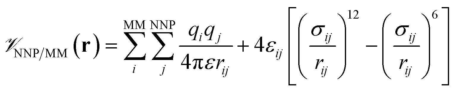 | (2) |
This functions similarly to mechanically-embedded QM/MM models,16 where the NNP serves as the “QM” model embedded within the MM system. This method can be employed in many established simulation codes without modification because they can implemented using existing QM/MM features, which allow the energy and forces of a critical subsection of the system to be calculated using an external method.
The immediate advantage of this method is that highly-accurate intramolecular forces can be calculated for ligands without parameterization and without modifications to current molecular simulation codes. A limitation of this approach is that the protein–ligand interactions are still calculated by the CGenFF/CHARMM electrostatic and Lennard-Jones terms. The development of efficient NNPs that are capable of describing the entire system could provide more accurate and non-empirical protein–ligand binding energies.
There have been several reports where QM/MM simulations were used to model protein–ligand complexes.17–19 The drawback of these QM methods is that typically they use semi-empirical quantum mechanics in order to calculate the energy and forces of the ligand sufficiently quickly to perform sufficiently long MD simulations. These methods generally are less accurate than the ANI NNPs for the calculations of the relative conformational stability of ligand conformations and the computational cost is generally greater. One advantage of QM/MM methods over the NNP/MM method used here is that the electron density of the ligand can be polarized by the protein and solvent (i.e., through electrostatic-embedding QM/MM16). This is not possible for the NNPs used here because these methods do make any calculation of the electron density of the ligand, so they are effectively mechanically embedded.
Technical details
All molecular dynamics (MD) simulations were performed using NAMD 2.13.20 The ligand intramolecular energies and forces were calculated using the ANI-1ccX14 NNP implemented in the TorchANI package.21 The programs were interfaced through the general-purpose external-force functionality of the NAMD QM/MM code.22 The CHARMM36m force field23 was used to represent the protein and the mTIP3P model24,25 was used to represent the water molecules. Sample input files and our scripts can be downloaded from our online repository26 and will be included in future distributions of NAMD. The CGenFF27 Lennard-Jones and electrostatic parameters were used to calculate the non-bonded ligand–protein interactions (i.e., ). Non-bonded interactions were calculated using a 12 Å cutoff, although lattice-summation methods are also available in the QM/MM NAMD interface.
The calculation of the erlotinib potential energy surface was performed using ORCA 4.2.1.28 Optimizations with constraints on the amine torsional angle were performed using the resolution of identity 2nd-order Møller–Plesset theory (RI-MP2) with the def2-TZVP basis set.29 Single point energy evaluations were performed at these optimized structures using Domain-based Local Pair Natural Orbital – Coupled Cluster Singles and Doubles with perturbative triples30 with the def2-TZVP basis set (DLPNO-CCSD(T)/def2-TZVP//RI-MP2/def2-TZVP) to generate the QM potential energy surface.
Test set
To evaluate the ability of the ANI-1ccX potential to predict the pose of a bound ligand, we developed a test set of protein–ligand complexes. We selected a structurally-diverse set of complexes where a high-resolution crystallographic structure of the protein–ligand complex was available, including several where the ligand is in a conformationally-strained pose. The ANI-1ccX NNP is only defined for carbon, nitrogen, hydrogen, and oxygen, so only ligands comprised of these elements were selected. The full details of the structures are included in the ESI.†Simulations of ligand binding poses
The NNP/MM ligand binding poses were generated by MD simulations of the protein–ligand complexes. The crystallographic structure (including crystallographic water molecules) was placed in a periodic unit cell of liquid water. The protonation states of the protein and ligand were assigned using H++ 3.2 (ref. 31) and by examining the intermolecular interactions of titratable residues in the crystallographic structure. A 5 ns equilibration MD simulation using the CGenFF force field for the ligand was performed where all non-hydrogen atoms of the ligand and protein were restrained to their crystallographic positions. The equilibrated structures were used as the initial structures of 2 ns NNP/MM MD simulations of the complexes. In these simulations, the Cα atom of the protein backbone were restrained to their crystallographic positions using harmonic potentials (kc = 10 kcal mol−1 Å−2). These simulations were performed with a thermostat temperature set to correspond to the temperature the crystallographic structure was collected for (e.g., 100 K). The ligand electron density was obtained from the crystallographic electron density map (2fo − fc), selecting all points within 2 Å of the ligand atoms in the PDB structure. An isosurface value of 0.5 was used in the renderings.Calculation of conformational Gibbs energy
Confine-and-release alchemical free energy perturbation is a popular technique for calculating absolute protein–binding energies.32–35 In these methods, the total binding energy is divided into a set of Gibbs energies for each step in a path where the ligand is constrained to its bound conformation and is then decoupled from its environment. The component corresponding to the reversible work required to constrain the ligand to its bound conformation is defined as ΔGcons. Physically, this energy corresponds to the reduction of conformational freedom and isomerization to a higher energy conformation that occurs when a ligand binds to a protein. In confine-and-release absolute binding energy calculation schemes, this is the only term where the intramolecular interactions of the ligand are significant. Accordingly, it is only necessary to use the NNP/MM method when calculating this term; the remaining terms can be calculated using conventional force fields. Notably, this step does not include any alchemical transformation, so performing the calculation with NNP/MM does not present any special challenges.This term can be calculated by defining the root-mean-square deviation (RMSD) of the ligand relative to its bound conformation (ζ) and then calculating the Gibbs energy required to impose a harmonic restraint on the RMSD 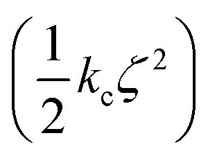 so that the ligand is restricted to hold its bound conformation. This procedure is performed for the ligand in solution and in the site to obtain Gibbs energies for restricting the conformation of the ligand in each of these states. The difference of these energies provides the conformational or “strain” component of the absolute binding energy (ΔGcons).
Using umbrella sampling, the potential of mean force (PMF) can be calculated as a function of the RMSD. Integration of this PMF biased by the harmonic restraining function provides the ΔGcons,site/solvent (eqn (3)).
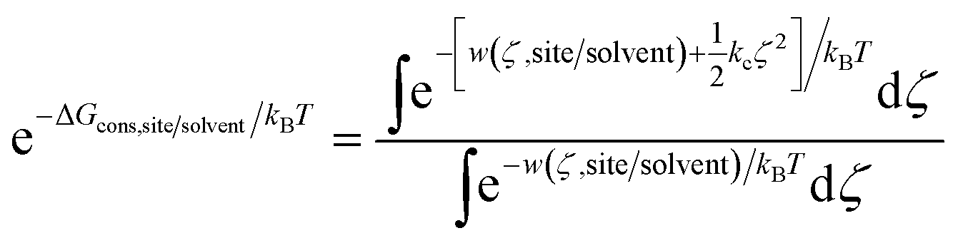 | (3) |
These PMFs are calculated from an umbrella sampling simulation where the windows were separated by 0.5 Å and a harmonic biasing potential with a spring constant of 50 kcal mol−1 Å−2 was used. Each window was sampled by performing a 1 ns equilibration simulation followed by a 4 ns sampling simulation. The PMF was constructed from the umbrella sampling simulations using Weighted Histogram Analysis Method (WHAM) with statistical uncertainties of the profiles estimated by bootstrap analysis.36–38
These calculations are performed for the ligand bound to the protein and in solution to yield ΔGcons,site and ΔGcons,solvent, respectively. The difference of these two energies provides ΔGcons (eqn (4)).
| ΔGcons = ΔGcons,site − ΔGcons,solvent | (4) |
Results and discussion
Prediction of ligand poses
Fig. 1 shows the ligand poses generated from the ANI/MD simulations overlaid with the crystallographic electron density maps of the ligand. Generally, the NNP/MM ligand pose overlaps well with the crystallographic density. The positions of the ligand phenyl rings in the thrombin complex (3DA9) and the biotin carboxylase complex (2W6N) are the most significant deviation. The NNP/MM model still relies on conventional MM parameters for the protein–ligand and water–ligand interactions, so these deviations may not be related to the NNP component of the model.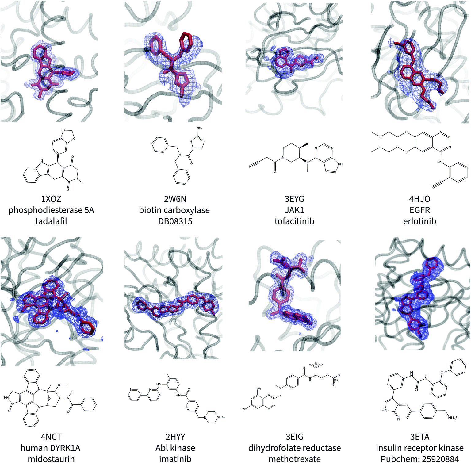 | ||
| Fig. 1 Calculated poses of ligands (red) in protein binding sites. The crystallographic electron density of the ligands are shown in blue. The PDB ID, protein name, and ligand name are included beneath the image. | ||
One notable success of the NNP/MM potential is in predicting the binding pose of erlotinib to the epidermal growth factor receptor (EGFR). The core scaffold of this drug is composed of amine-linked ethynyl-phenyl and quinazoline rings. Crystallographic structures of the protein-bound complex show the quinazoline ring bound in the adenosine-binding site while the ethynyl-phenyl group binds in a pocket formed by the T702, T830, and K721 residues. The binding pose predicted by CGenFF is inconsistent with the XRD data, in which the two rings form a more acute angle relative to each other (ϕ1 = 63 ± 1°, ϕ2 = 4 ± 1°). The simulation using the NNP/MM model is more consistent with the crystallographic data, (ϕ1 = 44 ± 1°, ϕ2 = 4 ± 1°).
Surprisingly, the poses predicted for the ligands that contain charged functional groups (2HYY, 3ETA, and 3EIG) are reasonable even though the ANI-1ccX potential was not designed to describe charged species and none of the molecules this NNP was trained for were charged.
Conformational free energies
The conformational strain of the ligand that occurs in protein–ligand binding arises from the need for the ligand to adopt the conformation it holds in its bound form. The bound conformation may be more strained than the lowest energy conformation it can hold in solution. Further, some ligands can adopt multiple conformations in solution, so limiting the conformational space of the ligand to the bound conformation is endergonic. For example, Roux and coworkers' calculations of the binding affinity of imatinib to Abl kinase predicted that while the net interaction energy of binding was −27.7 kcal mol−1, the conformational energy countered this by 11.3 kcal mol−1.39 The conformational energies for the test set of ligands were estimated by calculating the PMF (w(z)) for the deviation from the bound pose using umbrella-sampling MD simulations with both the CGenFF and NNP/MM models. ΔGcons was calculated from these PMFs using eqn (3). These energies are collected in Table 1. The PMFs for all complexes are presented in the ESI.†Amongst the neutral ligands, the NNP/MM conformational energies are generally similar in magnitude to the CGenFF strain energies. This indicates that the ANI-1ccX model can achieve similar results to the CGenFF model despite the lack of any explicit parameterization for these molecules. The conformational energies of 4HJO (erlotinib bound to EGFR) show the largest difference, with the NNP/MM strain energy being 4.7 kcal mol−1 smaller than the CGenFF strain energy. The high strain predicted by the CGenFF model is due to the amine functional group of erlotinib holding a pyramidal geometry in the solution simulations, creating a large energetic penalty to force the drug into its bound conformation. In the NNP/MM simulation of erlotinib in solution, the amine group remains close to a co-planar geometry with respect to the quinazoline ring, with a moderate skew in the dihedral angle between the phenyl group and the amine.
The ligands that contain charged functional groups (2HYY, 3ETA, and 3EIG) have anomalously high conformational energies. This issue originates from the use of the ANI-1ccX NNP, which was only trained on neutral molecules. This NNP predicts reasonable geometries of the ammonium and carboxylate groups in these molecules, but these ionic functional groups form spurious intramolecular contacts in the solution NNP/MM MD simulations. For example, the ligand of 3EIG adopts a conformation where the carboxylates groups are in close contact, rather than repelling each other like they should (see ESI†). This results in the stabilization of regions of the PMF corresponding to large structural deviations from the bound pose. As the NNP(ANI-1ccX) model was not designed for the description of charged molecules like this, it is unsuitable for calculating their conformational energies.
Extensive MD simulations are needed to calculate ΔGcons by calculating the PMF of the RMSD, but these simulations were completed at a modest computational cost because of efficient implementations of the ANI model for execution on graphical processing units (GPUs). For example, the NNP/MM MD simulations of imatinib (69 atoms) executed at a rate of 3.4 ns per day on a single Titan Xp NVIDIA GPU. Even faster performance is anticipated after the planned integration of NNPs directly into NAMD and other molecular simulation codes.
Empirical force fields are parameterized in an internally consistent manner, so it is possible that the MM parameters used to describe the non-bonded interactions between the ligand and its surroundings will not be optimal for the NNP/MM term. In particular, the balance between the MM ligand–water, ligand–protein, and the NNP ligand intramolecular dispersion interactions will not necessarily be consistent.3,4 This issue has been addressed in some QM/MM models by defining new parameters for the QM–MM Lennard-Jones terms.40,41 Nevertheless, the common practice has been to parameterize the intramolecular terms of ligands to gas phase potential energy surfaces, so the ANI-1ccX should a suitable replacement for these terms. If there were a serious inconsistency between the NNP and MM interaction energies, it would likely lead to a systematic difference in the conformational energies of the ligands, but the CGenFF and NNP/MM conformational energies are in close in magnitude for 1XOZ, 2W6N, 3EYG, and 4NCT.
Torsional potential energy surface of erlotinib
The large difference in the ANI-1ccX and CGenFF conformational energies of 4HJO (erlotinib bound to EGFR) originate from the ligand adopting conformations in solution that are drastically different than the bound conformation when the CGenFF model is used, while the NNP/MM model predicts similar conformations in both the binding site and solution. This is evident in the CGenFF PMF of the ligand's conformation relative to its bound pose in Fig. 2, which is considerably broader than the NNP/MM PMF and is higher energy in the crystallographic pose (RMSD = 0 Å).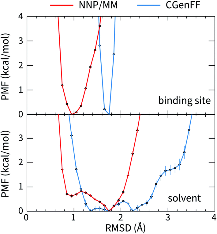 | ||
| Fig. 2 The potential of mean force for the deviation of the structure of erlotinib from its bound conformation when it is bound to EGFR (top, PDB ID: 4HJO) and when it is in solution (bottom) calculated using the hybrid NNP/MM and pure MM(CGenFF) methods. | ||
The geometry of the erlotinib amine linker and its aromatic substituents deviates sharply from the bound pose in the CGenFF solution structure (Fig. 3(b)); the amine is partially pyramidalized and the aromatic substituents are skew to each other. In contrast, in the NNP/MM simulation, the amine predominantly remains in a planar geometry, conjugated with the quinazoline and phenyl rings.
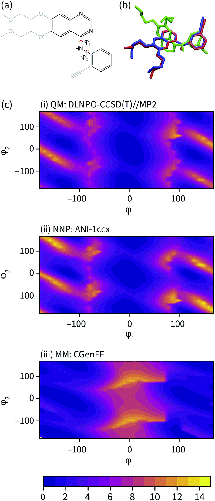 | ||
| Fig. 3 (a) The fragment of erlotinib used to calculate the potential energy surface. Truncated groups are shown in grey. (b) Representative solution conformations of erlotinib for the CGenFF MM model (green) and NNP/MM model (red) overlaid with the ligand pose from the 4HJO crystal structure. (c) The relaxed potential energy surfaces for rotation around the erlotinib fragment amine bonds calculated using (i) DLPNO-CCSD/def2-TZVP//MP2/def2-TZVP (ii) NNP(ANI-1ccX) and (iii) the CGenFF MM model. Energies are in kcal mol−1. | ||
The potential energy surface corresponding to rotations around the amine torsion angles of erlotinib is presented in Fig. 3(c). The minima on the CGenFF surface corresponds to structures where the amine is significantly pyramidal and the substituent phenyl and quinazoline rings adopt angles that reduce steric repulsion between them. The ANI-1ccX surface is consistent with the DLPNO-CCSD(T) surface, where there is a broad global minimum centered around ϕ1 = 0°, ϕ2 = 0° and the amine nitrogen holds a planar arrangement with the aromatic groups.
The failure of the CGenFF force field stems from the lack of a distinct atom type for amines conjugated with aromatic rings. While it would be possible to adjust the parameters of the CGenFF force field to improve its description of the arylamine potential energy surfaces, this introduces a new fitting stage and requires computationally demanding QM calculations to provide the target data. Generally, it is not immediately apparent where a general-purpose force field will fail. By using NNPs to calculate these interactions, these issues are avoided entirely because energy surfaces with near-CCSD(T) accuracy can be generated efficiently and without the need to parameterize the intramolecular potential energy surface explicitly.
Conclusions
NNPs provide accurate representations of the intramolecular interactions of drug molecules in molecular simulations of protein–ligand binding. These simulations take advantage of established MM models of the protein and solution, while eliminating the need to develop a force field for the intramolecular interactions of each ligand. By employing a NNP that has already been trained on a broad set of molecular species, the fundamental intramolecular interactions that give rise to the molecular energy surface are captured without the need to parameterize a force field. This representation is also free of the harmonic/torsional/improper terms used in conventional force fields. This allows the simulations to be deployed immediately, without the development of parameters for each new chemical moiety.These methods can be incorporated directly into existing confine-and-release methods to calculate the absolute binding energy because these methods include a step where the ligand's conformation is constrained to its bound pose. In several cases, the conformational energies calculated using the NNP(ANI-1ccX)/MM model were similar to those predicted by the popular general-purpose CGenFF force field.
The scope of the ligands that can be modelled is limited by the choice of the NNP, which is particularly true for the ANI-1ccX model. Firstly, the ANI-1ccX model only supports molecules containing C, N, O, and H, although many important drug molecules also contain sulfur, phosphorus, boron, or halogen atoms. Secondly, ANI-1ccX NNP was not designed for modeling ionic species. Although the binding poses predicted for these compounds were reasonable, the NNP spuriously favored high-energy conformations in solution. This reflects that the ANI-1ccX training data did not include ionic species. ANI-type models that are trained to describe molecules containing sulfur and halogens, as well as charged molecules, are currently in development.42
Conflicts of interest
There are no conflicts to declare.Acknowledgements
The authors thank NSERC of Canada for funding through the Discovery Grants program (RGPIN-05795-2016). SLJL thanks the School of Graduate Studies at Memorial University for a graduate fellowship, the Faculty of Science of Memorial University for a Science Undergraduate Research Award, and Dr Liqin Chen for a scholarship. Computational resources were provided by Compute Canada (RAPI: djk-615-ab). We gratefully acknowledge the support of NVIDIA Corporation with the donation of the Titan Xp GPU used for this research. CNR thanks the Beckman Institute at the University of Illinois for a travel grant.Notes and references
- K. Vanommeslaeghe, E. P. Raman and A. D. MacKerell, J. Chem. Inf. Model., 2012, 52, 3155–3168 CrossRef CAS PubMed.
- M. Riquelme, A. Lara, D. L. Mobley, T. Verstraelen, A. R. Matamala and E. Vöhringer-Martinez, J. Chem. Inf. Model., 2018, 58, 1779–1797 CrossRef CAS PubMed.
- M. Mohebifar, E. R. Johnson and C. N. Rowley, J. Chem. Theory Comput., 2017, 13, 6146–6157 CrossRef CAS PubMed.
- E. T. Walters, M. Mohebifar, E. R. Johnson and C. N. Rowley, J. Phys. Chem. B, 2018, 122, 6690–6701 CrossRef CAS PubMed.
- S. Lifson and A. Warshel, J. Chem. Phys., 1968, 49, 5116–5129 CrossRef CAS.
- E. Harder, W. Damm, J. Maple, C. Wu, M. Reboul, J. Y. Xiang, L. Wang, D. Lupyan, M. K. Dahlgren and J. L. Knight, et al. , J. Chem. Theory Comput., 2016, 12, 281–296 CrossRef CAS PubMed.
- L. Huang and B. Roux, J. Chem. Theory Comput., 2013, 9, 3543–3556 CrossRef CAS PubMed.
- L.-P. Wang, T. J. Martinez and V. S. Pande, J. Phys. Chem. Lett., 2014, 5, 1885–1891 CrossRef CAS.
- C. G. Mayne, J. Saam, K. Schulten, E. Tajkhorshid and J. C. Gumbart, J. Comput. Chem., 2013, 34, 2757–2770 CrossRef CAS PubMed.
- L. S. Dodda, I. Cabeza de Vaca, J. Tirado-Rives and W. L. Jorgensen, Nucleic Acids Res., 2017, 45, W331–W336 CrossRef CAS PubMed.
- M. Stroet, B. Caron, K. M. Visscher, D. P. Geerke, A. K. Malde and A. E. Mark, J. Chem. Theory Comput., 2018, 14, 5834–5845 CrossRef CAS PubMed.
- J. Behler, Angew. Chem., Int. Ed., 2017, 56, 12828–12840 CrossRef CAS PubMed.
- J. S. Smith, O. Isayev and A. E. Roitberg, Chem. Sci., 2017, 8, 3192–3203 RSC.
- J. S. Smith, B. T. Nebgen, R. Zubatyuk, N. Lubbers, C. Devereux, K. Barros, S. Tretiak, O. Isayev and A. E. Roitberg, Nat. Commun., 2019, 10, 2903 CrossRef PubMed.
- J. Behler and M. Parrinello, Phys. Rev. Lett., 2007, 98, 146401 CrossRef PubMed.
- D. Bakowies and W. Thiel, J. Phys. Chem., 1996, 100, 10580–10594 CrossRef CAS.
- M. P. Gleeson and D. Gleeson, J. Chem. Inf. Model., 2009, 49, 670–677 CrossRef CAS PubMed.
- Z. Fu, X. Li and K. M. Merz Jr, J. Comput. Chem., 2011, 32, 2587–2597 CrossRef CAS PubMed.
- K. D. Dubey and R. P. Ojha, J. Biol. Phys., 2011, 37, 69–78 CrossRef CAS PubMed.
- J. C. Phillips, R. Braun, W. Wang, J. Gumbart, E. Tajkhorshid, E. Villa, C. Chipot, R. D. Skeel, L. Kalé and K. Schulten, J. Comput. Chem., 2005, 26, 1781–1802 CrossRef CAS PubMed.
- Roitberg Group, TorchANI, 2019, https://github.com/aiqm/torchani Search PubMed.
- M. C. R. Melo, R. C. Bernardi, T. Rudack, M. Scheurer, C. Riplinger, J. C. Phillips, J. D. C. Maia, G. B. Rocha, J. V. Ribeiro and J. E. Stone, et al. , Nat. Methods, 2018, 15, 351–354 CrossRef CAS PubMed.
- J. Huang, S. Rauscher, G. Nawrocki, T. Ran, M. Feig, B. L. de Groot, H. Grubmüller, J. MacKerell and D. Alexander, Nat. Methods, 2017, 14, 71–73 CrossRef CAS PubMed.
- W. L. Jorgensen, J. Chandrasekhar, J. D. Madura, R. W. Impey and M. L. Klein, J. Chem. Phys., 1983, 79, 926–935 CrossRef CAS.
- E. Neria, S. Fischer and M. Karplus, J. Chem. Phys., 1996, 105, 1902–1921 CrossRef CAS.
- C. Rowley, NAMD–TorchANI interface scripts, 2019, https://github.com/RowleyGroup/NNP-MM Search PubMed.
- K. Vanommeslaeghe, E. Hatcher, C. Acharya, S. Kundu, S. Zhong, J. Shim, E. Darian, O. Guvench, P. Lopes, I. Vorobyov and A. D. Mackerell Jr, J. Comput. Chem., 2010, 31, 671–690 CAS.
- F. Neese, Wiley Interdiscip. Rev.: Comput. Mol. Sci., 2012, 2, 73–78 CAS.
- F. Weigend and R. Ahlrichs, Phys. Chem. Chem. Phys., 2005, 7, 3297–3305 RSC.
- Y. Guo, C. Riplinger, U. Becker, D. G. Liakos, Y. Minenkov, L. Cavallo and F. Neese, J. Chem. Phys., 2018, 148, 011101 CrossRef PubMed.
- R. Anandakrishnan, B. Aguilar and A. V. Onufriev, Nucleic Acids Res., 2012, 40, W537–W541 CrossRef CAS PubMed.
- J. Wang, Y. Deng and B. Roux, Biophys. J., 2006, 91, 2798–2814 CrossRef CAS PubMed.
- D. L. Mobley, J. D. Chodera and K. A. Dill, J. Chem. Theory Comput., 2007, 3, 1231–1235 CrossRef CAS PubMed.
- D. L. Mobley and K. A. Dill, Structure, 2009, 17, 489–498 CrossRef CAS PubMed.
- J. C. Gumbart, B. Roux and C. Chipot, J. Chem. Theory Comput., 2013, 9, 3789–3798 CrossRef CAS PubMed.
- S. Kumar, J. M. Rosenberg, D. Bouzida, R. H. Swendsen and P. A. Kollman, J. Comput. Chem., 1992, 13, 1011–1021 CrossRef CAS.
- B. Roux, Comput. Phys. Commun., 1995, 91, 275–282 CrossRef CAS.
- A. Grossfield, WHAM: the weighted histogram analysis method, version 2.0.6, 2018, http://membrane.urmc.rochester.edu/content/wham Search PubMed.
- Y.-L. Lin, Y. Meng, W. Jiang and B. Roux, Proc. Natl. Acad. Sci. U. S. A., 2013, 110, 1664–1669 CrossRef CAS PubMed.
- P. M. Zimmerman, M. Head-Gordon and A. T. Bell, J. Chem. Theory Comput., 2011, 7, 1695–1703 CrossRef CAS PubMed.
- C. N. Rowley and B. Roux, J. Chem. Theory Comput., 2012, 8, 3526–3535 CrossRef CAS PubMed.
- O. Isayev, personal communication.
Footnote |
| † Electronic supplementary information (ESI) available: Details of crystallographic structures and example NNP/MM NAMD input file. See DOI: 10.1039/c9sc06017k |
| This journal is © The Royal Society of Chemistry 2020 |