 Open Access Article
Fault diagnosis in a current sensor and its application to fault-tolerant control for an air supply subsystem of a 50 kW-Grade fuel cell engine
Rui Quan *ab,
Fan Wub,
Chengji Wangb,
Baohua Tanc and
Yufang Changa
aHubei Key Laboratory for High-efficiency Utilization of Solar Energy and Operation Control of Energy Storage System, Hubei University of Technology, Wuhan 430068, China. E-mail: quan_rui@126.com
bAgricultural Mechanical Engineering Research and Design Institute, Hubei University of Technology, Wuhan 430068, China
cSchool of Science, Hubei University of Technology, Wuhan, 430068, China
First published on 31st January 2020
Abstract
The safety, reliability and stability of air supply subsystems are still problems for the commercial applications of fuel cells; therefore, engine fault diagnosis and fault-tolerant control are essential to protect the fuel cell stack. In this study, a fault diagnosis and fault-tolerant control method based on artificial neural networks (ANNs) has been proposed. The offline ANN modification model was trained with a Levenberg–Marquardt (LM) algorithm based on other sensors' signals relevant to the current sensor of a 50 kW-grade fuel cell engine test bench. The output current was predicted via the ANN identification model according to other relevant sensors and compared with the sampled current sensor signal. The faults in the current sensor were detected immediately once the difference exceeded the given threshold value, and the invalid signals of the current sensor were substituted with the predictive output value of the ANN identification model. Finally, the reconstructed current sensor signals were sent back to a fuel cell controller unit (FCU) to adjust the air flow and rotate speeds of the air compressor. Experimental results show that the typical faults in the current sensor can be diagnosed and distinguished within 0.5 s when the threshold value is 15 A. The invalid signal of current sensor can be reconstructed within 0.1 s. Which ensures that the air compressor operate normally and avoids oxygen starvation. The proposed method can protect the fuel cell stack and enhance the fault-tolerant performance of air supply subsystem used in the fuel cell engine, and it is promising to be utilized in the fault diagnosis and fault-tolerant control of various fuel cell engines and multiple sensor systems.
1. Introduction
Green energy is a good alternative to alleviate the worldwide environmental and resource issues. Owing to high efficiency, no noise and zero pollution, the fuel cells have been considered as one of the future promising energy sources.1–3 Among the various fuel cells, the proton exchange membrane fuel cell (PEMFC) technology has been a research and commercialization focus in the stationary, mobile and transportation applications for its high-power density and efficiency, low operating temperature, and a quick response to the load.4–6 In recent years, the famous commercialized vehicles, such as “Mirai” of Toyota, “Clarity” of Honda, “ix35” and “NEXO” of Hyundai, have validated the sufficient performances of PEMFC for transportation applications with power of up to 100 kW. However, there are still some challenges such as lifetime, durability, costs, reliability, safety, and maintenance for fuel cells to overcome in commercial applications.7,8 Moreover, reliability and durability are the two main barriers, which impede its wide applications.In practical applications, improper operating conditions such as reactant starvation, flooding and drying may severely deteriorate the fuel cell performance, usually resulting in several single cell voltage drop. If the improper faulty conditions are recurrent or continue for a long period, other degradation phenomena may take place and accelerate the fuel cell stack ageing or even damage.9 Consequently, the fuel cell faults should be detected as early as possible. Among the solutions, fault diagnosis and fault-tolerant control, dedicated to detecting, isolating, reconstructing and analyzing different faults, are indispensable to keep the fuel cell stack operate safely and avoid mistakes in the control strategies of the fuel cell engine, which reduces downtime and mitigates performance degradation of the fuel cell stack.10–12
The fuel cell system (or called fuel cell engine) consists of multiple auxiliary subsystems other than fuel cell stacks, such as the air supply subsystem, hydrogen supply subsystem, cooling subsystem, electrical circuit and controller. As the air supply quantity is controlled according to the real output current value of the fuel cell stack, the majority of sensors may be affected by the severe electromagnetic interference (EMI) environment because of the high rotating speed, vibration and noise of air compressor, or common-mode and different-mode signals caused by other electrical components. Once the faults of the air supply subsystem occur without any detection, neither protective nor fault-tolerant control measures are taken in time, it will result in a shutdown, oxygen starvation or even permanent damage to the costly fuel cell stack. Thus, it is essential to study the fault diagnosis and fault-tolerant control for the fuel cell system, particularly for the current sensor used in the air supply subsystem.
The popular fault diagnosis approaches for the sensors include those based on hardware redundancy, Kalman filter, signal processing, neural networks and so on.13–17 The hardware redundancy-based method demands additional sensors to measure the same variable, but it will increase the complexity and costs of the fuel cell system. The Kalman filter is a promising method in the real time fault diagnosis of sensors for it can describe their dynamic performance,13 but the diagnosis performance mainly depends on the accurate mechanism models. In fact, the accurate mechanism models for different sensors are difficult to set up even though the accurate models during a certain time can be acquired. The accuracy may slowly decline, or the object parameters fluctuate as time flies. The signal processing method, particularly the wavelet analysis,14,15 is suitable for the signal singularity identification of the sensors; however, the output load of the fuel cell engine varies all the time and all the parameters of the fuel cell engine keep changing accordingly. Therefore, it is deficient to the fault diagnosis of sensors only by detecting sudden changes in their output signals.
Artificial neural networks (ANN) have an excellent ability of non-linear mapping and self-learning, and it can avoid the negative influence and subjective factors of the established unfaithful models.16,17 Therefore, ANN is applicable to the fault diagnosis of the complicated non-linear systems. In this study, the neural network trained with the Levenberg–Marquardt (LM) algorithm is utilized in the fault diagnosis of a current sensor and active fault-tolerant control for the air supply subsystem of a 50 kW-grade fuel cell engine designed by our group.
2. Schematic of the fuel cell engine
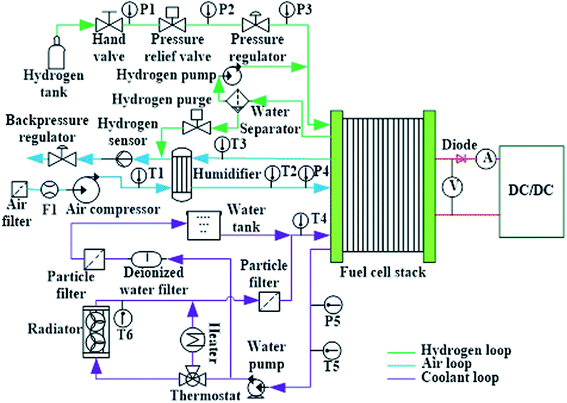
The detailed schematic of the 50 kW-grade fuel cell engine is shown in Fig. 1, and it includes a hydrogen supply subsystem, an air supply subsystem, a cooling subsystem and a fuel cell stack. The hydrogen subsystem consists of a hydrogen tank, a hand valve, a pressure relief valve, a pressure regulator, a hydrogen pump, a water separator, a hydrogen purge and several pressure sensors (P1 denotes the hydrogen tank pressure, P2 denotes the hydrogen relief pressure and P3 denotes the inlet hydrogen pressure); the air supply subsystem includes an air filter, an air compressor, a humidifier, a backpressure regulator, a hydrogen sensor (detecting hydrogen concentration) and several air sensors (F1 denotes the air flow sensor, T1 denotes the outlet temperature of air compressor, T2 and T3 denote the inlet and outlet air temperature, respectively, and P4 denotes the inlet air pressure); the cooling subsystem includes a radiator, a water tank, a thermostat, a particle filter, a deionized water filter, a heater, a water pump and several coolant sensors (T4 denotes the inlet coolant temperature, T5 denotes the outlet coolant temperature, T6 denotes radiator's outlet temperature and P5 denotes the coolant pressure). The output of the fuel cell engine is connected with a voltage sensor (denoted as V) in parallel and a current sensor (denoted as A) in series. The output power of the fuel cell engine is freely adjusted by the DC/DC converter.18According to the basic electrochemical reaction equation of the fuel cell, the required hydrogen and air flow are controlled by a fuel cell controller unit (FCU) according to the output current of the fuel cell engine. The required hydrogen flow and air flow are calculated as follows:19
 | (1) |
| FAir = 100/21 × 0.5 × FH2× λ = 0.0166λIn | (2) |
![[thin space (1/6-em)]](https://www.rsc.org/images/entities/char_2009.gif) 485), and λ is the excess air ratio (usually is 2).
485), and λ is the excess air ratio (usually is 2).
According to the above equations, when an error occurs in the current sensor, the required air flow will be out of control, particularly when the sampled value of the current sensor is much smaller than the practical value. If the air supply flow is controlled based on the inaccurate sampled value, the dangerous “oxygen starvation” fault occurs quickly with a large output power, it may also lead to irreversible damage to the fuel cell stack. Thus, the fault diagnosis and prediction of the current sensor used in the air supply subsystem is important. To enhance the robust performance of the fuel cell engine, the fault signal of the current sensor should be reconstructed with other relevant sensor signals.
3. Fault diagnosis and fault-tolerant control strategy
3.1. Diagnosis and signal reconstruction approach
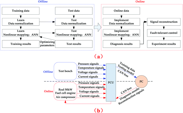
The proposed fault diagnosis and fault-tolerant control strategy are shown in Fig. 2, and the artificial neural network is trained and tested offline based on the sensor signals from the test bench, and the ANN parameters are optimized with the test results. The trained ANN model is used online for the fault diagnosis and signal reconstruction of the current sensor.In the offline process, the pressure, temperature, voltage and current signals of the above sensors are sampled with the A/D circuit of FCU, and saved as training and test data into a supervisory personal computer with a controller area network (CAN) bus. Then, the diagnosis model is trained using the supervisory personal computer (PC) and programmed with Python language. In the specific online stage, the real-time data are measured and processed using a PC with the trained offline model. The variability of the current sensor is predicted by the established ANN model according to other relevant sensors (such as pressure sensors, voltage sensors and temperature sensors) and compared with the practically sampled current signal. Once the compared result (i.e. the absolute error) is above the given threshold value, the fault of the output current sensor is validated, its practically sampled signal is substituted by the predicted value of the ANN model, and the required air flow is controlled by FCU based on the reconstructed value.
3.2. Training of ANN
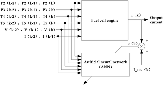
According to the above schematic of the designed fuel cell engine, it can be seen that the output current sensor value is relevant to the voltage sensors, the hydrogen pressure sensors and the coolant temperature sensors. Thus, the designed ANN model identification structure of a fuel cell engine is shown in Fig. 3. The hydrogen relief pressure (P2(k − 2), P2(k − 1), P2(k)), inlet hydrogen pressure (P3(k − 2), P3(k − 1), P3(k)), inlet coolant temperature (T4(k − 2), T4(k − 1), T4(k)), outlet coolant temperature (T5(k − 2), T5(k − 1), T5(k)), output voltage (V(k − 2), V(k − 1), V(k)) and output current (I(k − 2), I(k − 1)) are treated as its input variables, and the output current of kth time (I(k)) is the output variable. The identification process of the ANN model is to ensure the error (denoted e(k)) between the real output current sensor of the fuel cell engine (denoted I(k)), and the predictive value of the ANN model (denoted I_ANN(k)) approaches the training goal based on different groups of input variables.The standard BP algorithm is useful to the forward ANN for it adjusts the weight value and threshold value to ensure the minimum sum of square error between the output value of ANN and the object value. However, it has disadvantages such as slow convergence and local minimum value. In this study, the Levenberg–Marquardt (LM) algorithm20,21 is adopted to improve the BP algorithm for its rapid convergence and high efficiency. If X(k) is the kth vector comprised of weight values and threshold values, then X(k+1) is calculated using eqn (3).
| X(k+1) = X(k) + ∩X | (3) |
According to newton algorithm,22 ∩X is given by
| ∩X = −|∇2E(x)|−1∇E(x) | (4) |
 | (5) |
| ∇E(x) = JT(x)e(x) | (6) |
| ∇2E(x) = JT(x)e(x) + S(x) | (7) |
 J(x) is the Jacobian matrix given by
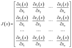 | (8) |
According to the Gauss–Newton algorithm,22 ∩X can be expressed as follows:
| ∩X = −[JT(x)J(x)]−1J(x)e(x) | (9) |
Moreover, according to the LM algorithm, ∩X can be rewritten by
| ∩X = −[JT(x)J(x) + μI′]−1J(x)e(x) | (10) |
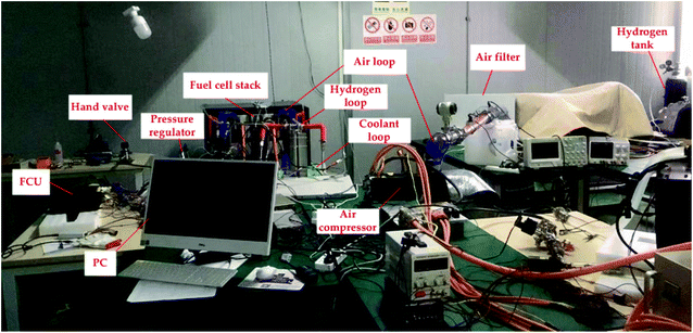
For the above ANN model identification structure, some experiments, in both normal operation and faulty cases, are carried out based on the fuel cell test bench, as shown in Fig. 4. In total, 1000 groups of different experimental data sets are obtained as the training sample, and another 200 different groups are selected as the test data. For the fuel cell engine test bench, the fuel cell stack includes two separate stacks connected in a series. Both of the stacks are manufactured by Ballard Power Systems Inc. (Model Name: FCvelocity-9SSL) and consist of 135 single fuel cells connected in a series.
During the test bench experiments, the output power of the fuel cell engine was controlled by an adjustable electronic load, the output current of the fuel cell engine was changed from 0 to 300 A, and all the data were recorded according to a time series. Due to the page limitation of this study, only some typical experimental data reflecting the rated power are provided in Table 1 on the training sample.
| Variables | Value 1 | Value 2 | Value 3 |
|---|---|---|---|
| P2(k − 2) | 670 kPa | 661 kPa | 652 kPa |
| P2(k − 1) | 661 kPa | 652 kPa | 650 kPa |
| P2(k) | 650 kPa | 649 kPa | 630 kPa |
| P3(k − 2) | 95 kPa | 96 kPa | 98 kPa |
| P3(k − 1) | 96 kPa | 98 kPa | 101 kPa |
| P3(k) | 98 kPa | 98 kPa | 138 kPa |
| T4(k − 2) | 58.2 °C | 58.6 °C | 58.8 °C |
| T4(k − 1) | 58.6 °C | 58.8 °C | 59.4 °C |
| T4(k) | 58.8 °C | 59.4 °C | 56.1 °C |
| T5(k − 2) | 67.1 °C | 67.7 °C | 67.9 °C |
| T5(k − 1) | 67.7 °C | 67.9 °C | 68.3 °C |
| T5(k) | 67.9 °C | 68.3 °C | 66.4 °C |
| V(k − 2) | 165.6 V | 158.2 V | 159.2 V |
| V(k − 1) | 161.5 V | 159.2 V | 158.2 V |
| V(k) | 159.2 V | 158.2 V | 158 A |
| I(k − 2) | 263 A | 276.3 A | 279.8 A |
| I(k − 1) | 276.3 A | 279.8 A | 280.8 A |
| I(k) | 279.8 A | 280.8 A | 294.1 A |
Due to the different orders of magnitude for the input and output variables, and to enhance the study efficiency of the ANN identification model, all the input and output variables are normalized using the following expression:
 | (11) |
 is the normalization value of input and output variables, xi is the real value, and xmax and xmin are the maximum and minimum values of variable x, respectively.
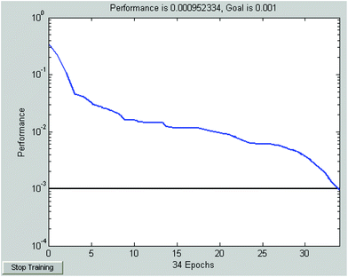
Fig. 5 gives the training result of the above ANN identification model with the LM algorithm. Based on the Kolmogorov theory,23 the final neuron number of the hidden layers is 13. The adopted neural networks function is “newff()”, the training function is “trainlm”, the hidden function is “tansig”, the output layer function is “logsig”, and the training goal is 0.001. It can be seen that the net converges to the goal after 34 epochs take about 1.4 s.
3.3. Testing of ANN
To evaluate the estimated performance of the ANN model, the root mean square error (RMSE) is adopted in this study and it is defined by24
 | (12) |
To describe the approximation degree between the target value of neural networks model and the output value of the neural networks model, variance account for (VAF) is given by25
 | (13) |
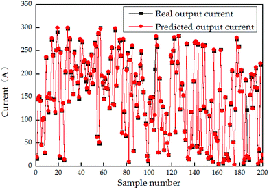
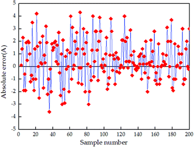
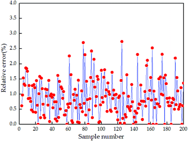
The comparison results between the 200 groups of the test data and the predicted output current value of the above established ANN identification model are presented in Fig. 6, and the corresponding absolute error and relative error are given in Fig. 7 and 8, respectively. Fig. 7 illustrates that the absolute error range between the real output current of the fuel cell engine (from 200 groups of the testing data) and predicted the output current value of the inverse normalization of the ANN identification model changes from −3.6 A to 4.2 A. The maximum relative error shown in Fig. 7 is 2.74%, and the average relative error shown in Fig. 8 is 0.91%.
To further analyze the performance of the established ANN identification model with the above LM algorithm, the traditional BP neural network model is also set up to compare with it based on the same training parameters. The overall comparison results are provided in Table 2. It demonstrates that the RMSE of the test data based on the traditional BP algorithm is 0.0048, while the one based on the LM algorithm for the same data is only 0.0031, which is decreased by 35.4%. Moreover, the VAF of the testing data with the LM algorithm is increased by 12.5% compared with that with the BP algorithm. Thus, it can be concluded that the established ANN identification model based on the LM algorithm has advanced predictive ability (the maximum predicted error is below 3%). The model is better than the traditional BP neural network model as the former model has much lower RMSE and larger VAF based on the same test sample.
| Algorithm type | Training data | Testing data | ||
|---|---|---|---|---|
| RMSE | VAF | RMSE | VAF | |
| BP | 0.0059 | 85.26 | 0.0048 | 82.94 |
| LM | 0.0042 | 94.13 | 0.0031 | 93.27 |
4. Experimental results and discussions
The above trained ANN diagnosis model was programmed with a PC and implemented online. According to the above schematic shown in Fig. 1, a 50 kW-grade real fuel cell engine for the city bus application is developed. Specific technical parameters (the same as test bench in Fig. 5) are provided in Table 3.| Parameter | Value |
|---|---|
| Active area of per cell | 286 cm2 |
| Stoichiometry H2 | 1.6 |
| Stoichiometry air | 2.0 |
| Maximum relief pressure | 850 kPa |
| Maximum inlet H2 pressure | 350 kPa |
| Maximum inlet air pressure | 200 kPa |
| Maximum coolant outlet temperature | 70 °C |
| Maximum allowable coolant temperature differential | 10 °C |
| Maximum allowable cross pressure-anode to coolant | 100 kPa |
| Maximum pressure differential between anode and cathode | 50 kPa |
| Maximum current | 300 A |
| Maximum allowable voltage | 230 V |
| Rated net power | 23 × 2 kW |
| Maximum power | 26.6 × 2 kW |
| Storage temperature | −40 °C to 60 °C |
| Start up temperature | >2 °C |
| Anode relative humidity | 95% |
| Cathode relative humidity | 95% |
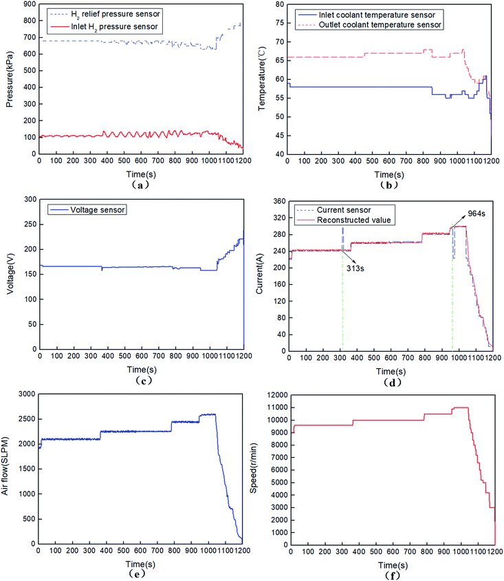
Fig. 9 illustrates the above experimental variables of a 50 kW-grade fuel cell engine under the major operations, which lasted for 1200 s and errors only occurred in the current sensor. At the 313th s, an error occurred in the fuel cell stack current sensor and caused a 58 A uprush (298.4 A) in the real current value (240.4). At the 313.5th s, the predicted current value of the ANN model was 243.4 A, and the difference between them exceeded the threshold (15 A). Based on the above strategy, it can be concluded that a sensor-level fault happened and the status of the fuel cell stack current sensor was abnormal. This error was detected at this moment and fed back to FCU by the PC with the CAN bus at the 313.9th second. The real current signal was reconstructed by FCU according to the received predicted value of the ANN model (i.e., 243.4 A). Then, the rotating speed of the air compressor was maintained at 9630 rpm by FCU, the corresponding air flow was 2179SLPM (i.e., 130.7 m3 h−1).
Furthermore, at the 964th s, another error occurred in the fuel cell stack current sensor and caused a 75 A drop (223.1) in the real current value (298.1 A). At the 964.5th s, the predicted current value of the ANN model was 298.3 A. As the difference also exceeded the given threshold value, this error was detected at this moment, and the fault signal of the current sensor was reconstructed by the predicted current value of the ANN model (i.e., 298.3 A) at the 964.9th s. As such, the rotating speed of the air compressor was maintained at 11![[thin space (1/6-em)]](https://www.rsc.org/images/entities/char_2009.gif) 020 rpm by FCU, the corresponding air flow was 2674SLPM (i.e., 160.4 m3 h−1). This can avoid the “oxygen starvation” damage in case the fault signal of the current sensor is treated as the real current value.
020 rpm by FCU, the corresponding air flow was 2674SLPM (i.e., 160.4 m3 h−1). This can avoid the “oxygen starvation” damage in case the fault signal of the current sensor is treated as the real current value.
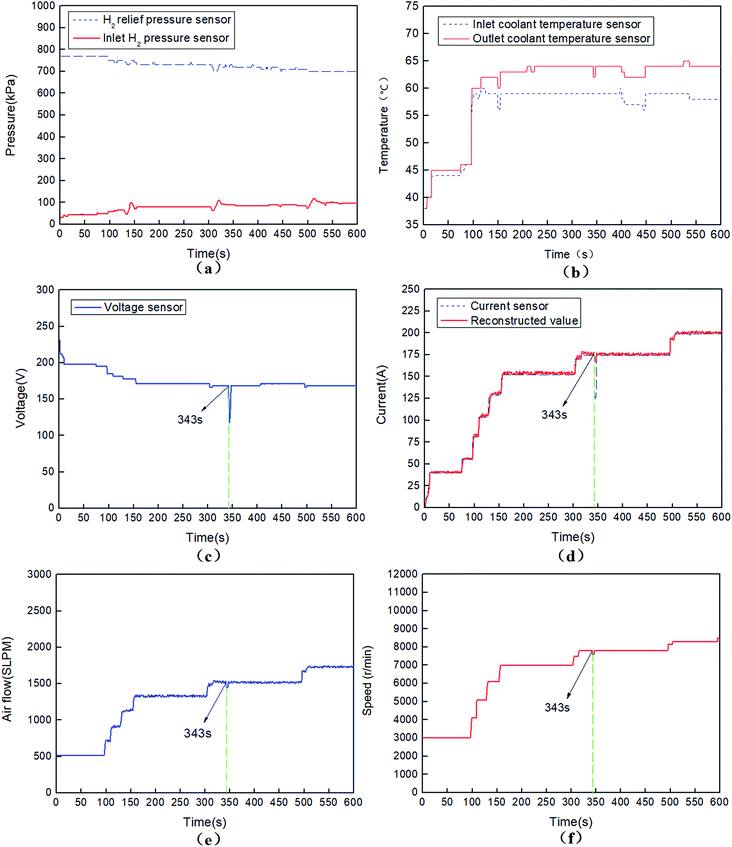
Fig. 10 illustrates the above experimental variables of a 50 kW-grade fuel cell engine under another operation, which lasted for 600 s and errors occurred both in the current sensor and voltage sensor simultaneously at the 343rd s. On this occasion, a 49 A dip (125.4 A) in the real current value (177.5 A) and a 39 V drop (129.1 V) in the real voltage value (168.1 V) occurred. At the 343.4th s, the predicted current value of the ANN model was 167.9 A, the difference between them also exceeded the threshold (15 A) value. A sensor-level fault and abnormal status of the fuel cell stack current sensor had been validated. This error was detected and sent back to FCU by a PC with the CAN bus at the 343.9th s, and the real current signal was reconstructed by FCU according to the received predicted value of the ANN model (167.9 A). Then, the rotating speed of the air compressor maintained at 7600 rpm was controlled by FCU, the corresponding air flow was 1451SLPM (i.e. 87.1 m3 h−1).
The required air flow is shown in Fig. 9(e) and 10(e), respectively. The corresponding controlled rotating speeds of the air compressor are shown in Fig. 9(f) and 10(f), respectively. Both the figures demonstrate that the air flow is directly proportion to the real output current, and the higher the rotating speed of the air compressor, the larger the air flow. When the error only occurs in a single current senor, the predictive value of the ANN identification model is in close proximity with the accurate value of the current sensor, and the predictive value can be treated as the reconstruction signal of the fault current sensor. When the errors occurred in the current sensor and another sensor simultaneously, the predictive value of the ANN identification model is a little different from the real accurate value of the current sensor, but the difference is acceptable, and the predictive value of the ANN identification model can also be treated as the reconstruction signal of the fault current sensor to some extent. The rotating speed of the air compressor is directly controlled according to the normal value of the current sensor, once errors occur in the current sensor, it will be adjusted by the reconstructed current signals of the ANN identification model. Overall, the above method ensures the fault-tolerance performance and reasonable control strategy of the air supply system of the fuel cell engine.
5. Conclusions
To ensure the safety and reliability of the fuel cell engine in the commercial fuel cell buses, a kind of fault diagnosis and fault-tolerant control approach for the air supply subsystem based on ANN has been proposed and designed. First, some sensor signals relevant to the current sensor were extracted from the test bench to train the offline ANN identification model with the LM algorithm. Second, the online fault diagnosis was designed based on a PC embedded with the offline ANN identification model and FCU.To verify the proposed method, two experiments involving errors occurring in a single current sensor as well as errors occurring in both, the current sensor and voltage sensor, were performed. During the experiments, when the difference between the current sensor signal and the predictive output value of the ANN model exceeds the given threshold value, the fault of the current sensor is detected within 1 s by the PC. Simultaneously, the invalid signals are substituted with the predictive output of the ANN identification model and sent back to FCU. The air flow and rotating speeds of the air compressor are controlled by FCU with the CAN bus based on the reconstructed current signals. Even though such errors during the above experiments will cause no serious damage to the fuel cell stack directly, but they may result in mistakes in the control strategies of the air supply subsystem (such as shut down of oxygen starvation). The above method has been applied in practical system for months, the experimental results show that it can quickly detect the current sensor signal value and immediately reconstruct the invalid current sensor signal by the predictive output of the ANN identification model. This method enhances the fault-tolerant control performance of the air supply subsystem and protects the fuel cell stack. It also provides an instructional alternative to the reliability, stability and safety research of other complicated non-linear systems with large numbers of sensors.
In the future study, efficient and reliable fault diagnosis and fault-tolerant control methods will be further researched and tested when multiple sensors (two or more) failures occur simultaneously.
Conflicts of interest
There are no conflicts to declare.Acknowledgements
This paper was supported by the National Natural Science Foundation of China (51977061, 61903129, 51407063).References
- A. Alaswad, A. Baroutaji, H. Achour, J. Carton, A. AlMakky and A. G. Olabi, Developments in fuel cell technologies in the transport sector, Int. J. Hydrogen Energy, 2015, 41, 499–508 Search PubMed.
- N. Majid and H. Mohammad, A new control strategy of solid oxide fuel cell based on coordination between hydrogen fuel flow rate and utilization factor, Renewable Sustainable Energy Rev., 2013, 27, 505–514 CrossRef.
- J. H. Jang, W. M. Yan, H. C. Chiu and J. Y. Lui, Dynamic cell performance of kW-grade proton exchange membrane fuel cell stack with dead-ended anode, Appl. Energy, 2015, 142, 8–14 CrossRef.
- J. O. Park, K. Kwon, M. D. Cho, S. G. Hong, T. Y. Kim and D. Y. Yoo, Role of binders in high temperature PEMFC electrode, J. Electrochem. Soc., 2011, 158, B675–B681 CrossRef CAS.
- C. H. Lin and S. Y. Tsai, An investigation of coated aluminium bipolar plates for PEMFC, Appl. Energy, 2012, 100, 87–92 CrossRef CAS.
- P. C. Dong, Y. X. Jia, G. N. Xie and M. Ni, The energy performance improvement of a PEM fuel cell with various chaotic flowing channels, Int. J. Energy Res., 2019, 43, 5460–5478 CrossRef CAS.
- J. Wang, Barriers of scaling-up fuel cells: cost, durability and reliability, Energy, 2015, 8, 509–521 CrossRef.
- N. Caqué, L. Flandin, C. Bas, G. D. Moor, A. Elkaddouri, E. Moukheiber, J. C. Perrin, A. Lamibrac, J. Dillet, G. Maranzana, O. Lottin, M. Chatenet, F. Maillard, L. Castanheira and L. Dubau, A review of PEM fuel cell durability: materials degradation, local heterogeneities of aging and possible mitigation strategies, Wiley Interdiscip. Rev.: Energy Environ., 2014, 3, 540–560 Search PubMed.
- Z. Zheng, R. Petrone, M. Pera, D. Hissel, M. Becherif, C. Pianese, N. Y. Steiner and M. Sorrentino, A review on non-model based diagnosis methodologies for PEM fuel cell stacks and systems, Int. J. Hydrogen Energy, 2013, 38, 8914–8926 CrossRef CAS.
- T. H. Lee, K. Y. Park, J. T. Kim, Y. Seo, K. B. Kim, S. J. Song, B. Park and J. Y. Park, Degradation analysis of anode-supported intermediate temperature-solid oxide fuel cells under various failure modes, J. Power Sources, 2015, 276, 120–132 CrossRef CAS.
- J. Q. Li, Z. Y. Hu, L. F. Xu, M. G. Ouyang, C. Fang, J. M. Hu, S. L. Cheng, H. Po, W. B. Zhang and H. L. Jiang, Fuel cell system degradation analysis of a Chinese plug-in hybrid fuel cell city bus, Int. J. Hydrogen Energy, 2016, 41, 295–310 CrossRef.
- W. Schmittinger and A. Vahidi, A review of the main parameters influencing long-term performance and durability of PEM fuel cells, J. Power Sources, 2008, 180, 1–14 CrossRef CAS.
- D. Kim and D. Lee, Fault Parameter Estimation Using Adaptive Fuzzy Fading Kalman Filter, Appl. Sci., 2019, 9, 3329 CrossRef.
- N. Y. Steiner, D. Hissel, P. Moçotéguy and D. Candusso, Non intrusive diagnosis of polymer electrolyte fuel cells by wavelet packet transform, Int. J. Hydrogen Energy, 2011, 36, 740–746 CrossRef CAS.
- J. Rafiee, M. A. Rafiee and P. W. Tse, Application of mother wavelet functions for automatic gear and bearing fault diagnosis, Expert Syst. Appl., 2010, 37, 4568–4579 CrossRef.
- G. Q. Li, C. Deng, J. Wu, X. B. Xu, X. Y. Shao and Y. H. Wang, Sensor Data-Driven Bearing Fault Diagnosis Based on Deep Convolutional Neural Networks and S-Transform, Sensors, 2019, 19, 2750 CrossRef PubMed.
- J. Kim, I. Lee, Y. Tak and B. H. Cho, State-of-health diagnosis based on hamming neural network using output voltage pattern recognition for a pem fuel cell, Int. J. Hydrogen Energy, 2012, 37, 4280–4289 CrossRef CAS.
- R. Quan, W. Zhou, G. Y. Yang and S. H. Quan, A hybrid maximum power point tracking method for automobile exhaust thermoelectric generator, J. Electron. Mater., 2017, 46, 2676–2683 CrossRef CAS.
- M. C. Williams, T. Horita, K. Yamagi, N. Sakai and H. Yokokawa, Basic Electrochemical Thermodynamic Studies of Fuel Cells and Fuel Cell Hybrids, J. Fuel Cell Sci. Technol., 2009, 6, G3152–G3158 Search PubMed.
- H. Zhao, R. X. Zhou and T. Q. Lin, Neural network supervised control based on Levenberg-Marquardt algorithm, J. Xi'an Jiaot. Univ., 2002, 36, 523–527 Search PubMed.
- X. G. Fu, S. H. Li, M. Fairbank, D. Wunshc and E. Alonso, Training recurrent neural networks with the Levenberg-Marquardt algorithm for optimal control of a grid-connected converter, IEEE Trans. Neural Netw. Learn. Syst., 2015, 26, 1900–1912 Search PubMed.
- S. S. Shamsudin and X. Q. Chen, Recursive Gauss-Newton based training algorithm for neural network modelling of an unmanned rotorcraft dynamics, Int. J. Intell. Syst. Technol. Appl., 2014, 13, 56–80 Search PubMed.
- A. N. Kolmogorov, On the representation of continuous functions of many variables by superposition of continuous functions of one variable and addition, Dokl. Akad. Nauk SSSR, 1957, 2, 953–956 Search PubMed.
- A. S. Korkhin, Estimating the matrix of root-mean-square errors of estimates of linear regression parameters for an arbitrary number of regressors and three inequality constraints, Cybern. Syst. Anal., 2006, 42, 342–356 CrossRef.
- W. H. Greene, D. A. Hensher and J. Rose, Accounting for heterogeneity in the variance of unobserved effects in mixed logit models, Transp. Res. Part B Methodol., 2006, 40, 75–92 CrossRef.
| This journal is © The Royal Society of Chemistry 2020 |

