Modelling water diffusion in plasticizers: development and optimization of a force field for 2,4-dinitroethylbenzene and 2,4,6-trinitroethylbenzene

Abstract

A classical all-atom force field has been developed for 2,4,6-trinitroethylbenzene and 2,4-dinitroethylbenzene and applied in molecular dynamics simulations of the two pure and two mixed plasticizer systems. Bonding parameters and partial charges were derived through electronic and geometry optimization of the single molecules. The other required parameters were derived from values already available in the literature for generic nitro aromatic compounds, which were adjusted to reproduce to a high level of accuracy the densities of 2,4-dinitroethylbenzene, 2,4,6-trinitroethylbenzene and the energetic plasticizers K10 and R8002. This force field has been applied to both K10 and R8002, which when used as plasticizers form an energetic binder with nitrocellulose. Nitrocellulose decomposes in storage, under varying conditions, but in particular where it may become increasingly dry. Following the derivation of the force field, we have therefore applied it to calculate water diffusion coefficients for each of the different materials at 298 K and 338 K, thereby providing a starting point for understanding water behaviour in a nitrocellulose binder.

---

1. Introduction

Nitrocellulose (NC) can be used as the explosive component in energetic material formulations such as propellants and polymer-based explosives (PBXs). Many fatal disasters are reported globally in relation to NC storage,^1,2 because NC decomposes over time which can lead to self-ignition. The likelihood of fire or even explosion is greatly increased when NC is dry, and during the entire period of storage and transport NC is therefore kept in a wetted condition with a wetting agent, the most common being isopropanol, ethanol or water.^3,4 Considering the high risk and danger of dry or partially dry NC, the interaction with water of NC and any other constituents in the energy material formulation, such as a plasticizer, whilst wetted and in storage is of significant importance. Industrial NCs are required by law to contain at least 25% wetting agent or 18% plasticizer.⁵ Both wetting agents and plasticizers act as phlegmatizers which stabilize or desensitize an explosive such as NC.⁵ As early as 1932, ethylbenzene nitro derivatives were known to be excellent colloiding agents for nitrocellulose.⁶ To further our understanding of the plasticizers used for NC, we have employed classical dynamics to investigate two common plasticizer mixtures and their interaction with water. A classical all-atom force field is parameterized for two materials, namely 2,4-dinitroethylbenzene (2,4-DNEB) and 2,4,6-trinitroethylbenzene (2,4,6-TNEB), which we have then applied to investigate water diffusion in the two pure systems 2,4-DNEB and 2,4,6-TNEB, as well as in the common plasticizer mixtures R8002 (50% 2,4-DNEB, 50% 2,4,6-TNEB) and K10 (65%, 2,4-DNEB, 35% 2,4,6-TNEB).^7,8

A number of studies using molecular dynamics (MD) simulations have investigated the properties of many of the different energetic material formulations available.^9–13 Essential for such simulations are suitable force fields for the explosive component and any additional constituents in the formulation, such as a plasticizer. Many of the force fields commonly used to model biomolecules and small organic molecules contain nitro group parameters,^14–17 but only very few force fields have been developed for specific nitro aromatic compounds.¹⁸ However, the combination of aromatic rings and nitro groups lead to complex structures, which require careful derivation of focussed forcefields as the more generic forcefields do not reproduce accurately the experimentally observed properties of these systems.

The force field for 2,4-DNEB and 2,4,6-TNEB was parameterized using an empirical method based on quantum mechanical calculations, literature values and experimental data. Bonding terms and partial charges were derived from the Hessian of quantum mechanical vibrational analysis calculations, whilst non-bonding terms were obtained from the refinement of literature values of similar molecules. Optimization was achieved by adjustment of parameters to reproduce the experimental densities of 2,4,6-TNEB and 2,4-DNEB and the plasticizer mixtures K10 (65% 2,4-DNEB and 35% 2,4,6-TNEB) and R8002 (50% 2,4,6-TNEB and 50% 2,4-DNEB).^7,8 The diffusion coefficients of 2,4,6-TNEB and 2,4-DNEB in K10 and R8002 were calculated along with the self-diffusion coefficients in the pure systems to evaluate if the interactions of 2,4,6-TNEB and 2,4-DNEB with themselves and in the mixtures were as expected considering the simulated densities. MD simulations of 2,4,6-TNEB, 2,4-DNEB, K10 and R8002 with water were performed at 298 K and 338 K for the calculation of the diffusion coefficients for water in these different systems. In a recent NC-related explosion, the temperature inside containers of wetted NC reached 338 K and we have therefore investigated the behaviour of water at this critical temperature compared to room temperature by calculating diffusion coefficients at 298 K and 338 K.¹⁹ The diffusion coefficients were calculated using both the Green–Kubo formula and the Einstein equation for comparison and an indication of their reliability.

2. Theoretical methods

2.1 Force field parameterization

The functional form of most classical force fields is shown in eqn (1).²⁰

The first two terms describe bond stretching and angle bending, where in our force field the equilibrium bond lengths, r_eq, and bond angles, θ_eq were taken directly from 2,4-DNEB and 2,4,6-TNEB structures, geometry-optimized by density functional theory (DFT) calculations, as shown in Fig. 1A to D. Our in-house software, based on a method devised by Seminario,^21,22 obtained internal force constants for bond stretching, K_r and angle bending, K_θ from Cartesian second derivatives (Hessian matrices) generated from the DFT frequency calculations. The majority of torsional angle parameters were taken from the General Amber Force Field (GAFF),²³ whereas the dihedral angle for C–C–C–N for nitrobenzene was taken from the literature.¹⁵ Out-of-plane deformation of the nitro group and rotation of the C–NO₂ bond in the aromatic ring of nitrotyrosine is apparent in X-ray structures.^24,25 In our forcefield, we have employed a proper dihedral for C–C–N–O and an improper dihedral for C–O–N–O, which is transferable to other nitro aromatic compounds and was developed specifically to model the out-of-plane deformation and rotation of the NO₂ group in nitrotyrosine.²⁶V_n describes the barrier height and γ the phase angle, as shown in the third term of eqn (1).²⁷ The final term describes the non-bonded interactions, where the first part is the Lennard Jones (LJ) 12–6 potential. In this functional form, the A_ij and B_ij parameters control the depth and position of the potential energy well for a pair of non-bonding interacting atoms where R_ij is the interatomic distance between the atoms.²⁰ Despite the lack of force fields for specific nitro-aromatic compounds, parameters for nitrobenzene are available. The LJ parameters for nitrobenzene were obtained from the OPLS force field and for aliphatic carbon and hydrogen atoms obtained from the GAFF and used as starting points before refining them for our systems.^17,23 The latter part of the final term represents the electrostatic potential, where q_i and q_j are the atomic partial charges and ε is the dielectric constant. The literature does not contain dielectric constants specifically for 2,4-DNEB and 2,4,6-TNEB. However, a value of 2.8 F m⁻¹ is available for 2,4,6-Trinitrotoluene (TNT),²⁸ and in view of the structural similarities of 2,4-DNEB and 2,4,6-TNEB to TNT, a dielectric constant of 2.8 F m⁻¹ was used for both molecules. The RED server development package was used to generate the partial charges using restricted electrostatic potential (RESP) charges from the DFT optimized 2,4-DNEB and 2,4,6-TNEB structures, displayed in Fig. 1E and F, respectively.^29–32

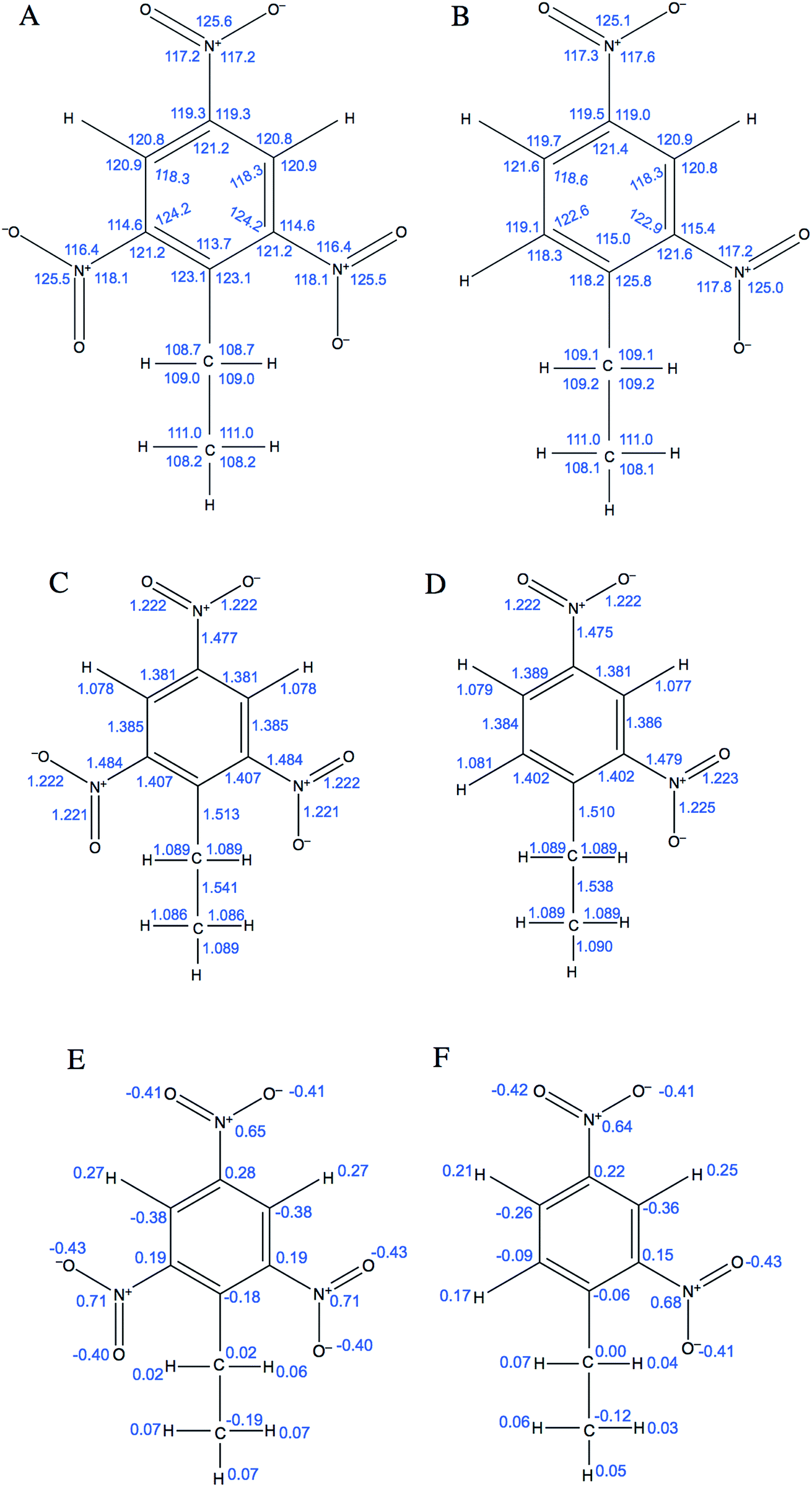Fig. 1 Equilibrium bond angles (A) and (B) and equilibrium bond lengths (C) and (D) for 2,4,6-TNEB and 2,4-DNEB, respectively. Partial charges for (E) 2,4,6-TNEB and (F) 2,4-DNEB.

2.2 Details of quantum mechanical calculations

Gaussian '09 was used for all DFT calculations,³³ with geometry optimizations followed by frequency calculations performed at the B3LYP/6-311⁺⁺G** level. Geometry optimization was achieved once the average root mean square (RMS) force on all atoms reached 0.01 kcal mol⁻¹ Å⁻¹, this criterion ensured adequate convergence and reliability of frequencies computed in a subsequent step for molecular systems that may have very small force constants. The absence of imaginary modes in the frequency calculations assured that the energy of each geometry optimized structure had reached an energy minimum.

2.3 Validation of parameters

The quantum mechanical (QM) bond angles and lengths obtained from the DFT optimized 2,4-DNEB and 2,4,6-TNEB structures were compared to experimental values for trinitrobenzene and ethylbenzene.^34–37 QM bonding terms in good agreement with experimental data were used in subsequent single molecule 2,4-DNEB and 2,4,6-TNEB MD simulations. Then, if dynamic bond lengths and angles of 2,4-DNEB and 2,4,6-TNEB from the single molecule MD simulations were comparable to experimental data,^34–37 simulations to test the entire parameter space were performed using the QM bonding terms. Chemical and physical properties of the liquid and solid phase were used for comparison between the force field parameterization and experimental data. Once full sets of force field parameters had been created for the 2,4-DNEB and 2,4,6-TNEB systems, their densities were calculated from MD simulations at 298 K. The LJ parameters were adjusted systematically until parameters were obtained that produced calculated densities from the MD simulations that were comparable to the experimental values.^38,39 Next, the densities of the plasticizer mixtures K10 and R8002 were simulated at 298 K, and the LJ parameters were adjusted until their simulated densities also agreed with experimental values.^7,40 Simulated densities were considered to be in good agreement with experiment if they were within ∼2% of the experimental values. In order to assess the performance of our force field, we have compared the densities of 2,4,6-TNEB and 2,4-DNEB obtained using our optimised force field with those obtained using the original LJ parameters before their adjustment, as well as with the densities obtained from a simulation where all parameters were taken from a published force field in the literature.^15,23,26 The published force field used torsional angles and original non-bonding parameters from the literature, as in our force field before optimisation (Section 2.1),^15,23,26 but all bonding terms were taken from the GAFF.²³ The 2,4,6-TNEB and 2,4-DNEB RESP partial charges obtained via our parameterisation method were used, as these are not readily available in GAFF and must be derived for a specific molecule via geometry optimisation.

2.4 Details of molecular dynamics simulations

All simulations were performed using the Sander module of the Amber 14 package.²⁰ For the solid and liquid simulations, periodic boundary conditions were defined for all three dimensions. A non-bonded cut-off of 8 Å was used for the pairwise Lennard-Jones interactions and the particle mesh ewald (PME) summation for the treatment of long-range electrostatics. Prior to the MD simulations, a minimization was performed to ensure molecules had adopted a conformation in a local minimum, where the steepest descent method was used initially, followed by a larger number of conjugate gradient cycles. Minimisation was halted when the RMS of the Cartesian element of the gradient was less than 1.0 × 10⁻⁴ kcal⁻¹ mol⁻¹ Å⁻¹. Bonds to hydrogen atoms were constrained using the SHAKE algorithm.⁴¹ The Velocity Verlet algorithm integrated the equations of motion and a 0.001 ps time step was used.⁴² The systems were heated to the temperatures required for the simulations. Constant temperature MD equilibration at constant volume (NVT) and constant pressure (NPT), followed by NPT production were performed using Anderson temperature-coupling and the Berendsen barostat was used to maintain constant pressure in the NPT simulations^43,44

2.5 Molecular systems

Details of the unit cell for 2,4-DNEB and 2,4,6-TNEB to use in the construction of the computational supercells for simulations at 298 K were unavailable, so information was used from the structurally similar compounds 2,4,6-trinitrotoluene (TNT) and 2,4-dinitrotoluene (2,4-DNT). To create the simulation box for 2,4,6-TNEB, experimental data were used of the monoclinic unit cell of TNT determined by Vrcelj et al.,⁴⁵ assuming a cubic geometry for the simulation box. The number of 2,4,6-TNEB molecules that could be added to a 40 ų cubic box was estimated from the unit cell volume of TNT and as such 238 2,4,6-TNEB molecules were added to a 40 ų simulation box. The monoclinic unit cell for 2,4-DNT reported by Hanson et al.⁴⁶ was used to create the simulation box for 2,4-DNEB, again assuming a cubic geometry. The same method outlined previously for 2,4,6-TNEB was used to add 283 2,4-DNEB molecules to a cubic 40 ų simulation box. For the plasticizer K10, a mixture of 144 2,4-DNEB molecules and 78 2,4,6-TNEB molecules was added to a 40 ų cubic box to make up a 65%/35% composition. A 1 : 1 mixture of 2,4-DNEB and 2,4,6-TNEB, i.e. 111 molecules of each, were added to a 40 ų cubic simulation box to make up the composition of plasticizer R8002. The program Packmol was used to build all simulation boxes, whereas all molecules were added with a tolerance of 2 Å (Fig. 2 and 3).⁴⁷

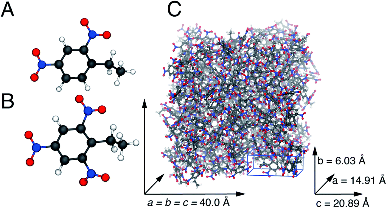Fig. 2 The geometry optimized 2,4-DNEB (A) and 2,4,6-TNEB (B) structures. The simulation cell for 2,4,6-TNEB (C), constructed from the TNT unit cell. Carbon atoms are displayed in grey, nitrogen atoms in blue, oxygen atoms in red and hydrogen atoms in white.

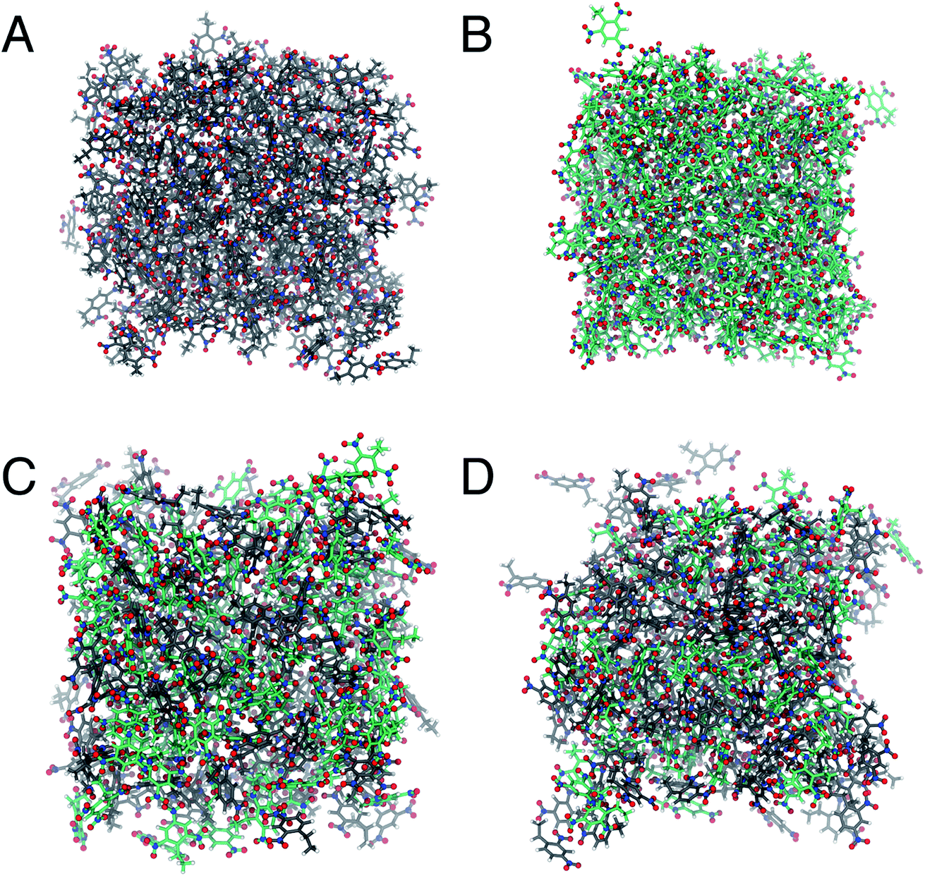Fig. 3 Representations of the simulation cells for (A) 2,4-DNEB, (B) 2,4,6-TNEB, (C) R8002 and (D) K10 at the end of MD production runs at 298 K. In all representations carbon atoms are displayed in grey, nitrogen atoms in blue, oxygen atoms in red and hydrogen atoms in white. The bonds in 2,4,6-TNEB are grey and those in 2,4-DNEB are green.

2.6 Molecular dynamics simulations

MD simulations of single molecules of 2,4-DNEB and 2,4,6-TNEB were performed in vacuum at 298 K for 3.5 ns. In order to measure the bond angles and lengths from the single molecule simulations, no constraints were applied, allowing bonds and angles to equilibrate. Snapshots were taken every 400 steps and average bond lengths and bond angles were calculated over the last 2 ns.

Simulations were performed at 298 K under vacuum of the pure 2,4-DNEB and 2,4,6-TNEB systems as well as the energetic plasticizer mixtures K10 and R8002. Each system underwent a 30 ps NVT equilibration, followed by a 400 ps NPT equilibration in order to stabilize the pressure and therefore the density. Finally, for each system a 12 ns NPT production run was performed before analysis. Diffusion coefficients calculated using the Green–Kubo (GK) formula are derived from the velocity autocorrelation function (VACF) which requires shorter simulations. To obtain the VACFs, simulations were performed on all systems using the above method, but production runs were 10 ps in length.

Unit cell dimensions and the number of 2,4-DNEB and 2,4,6-TNEB molecules used for the simulations with water were the same as those used in simulating the pure systems and plasticizer mixtures. Wetted nitrocellulose in plasticized energetic material formulations typically contains at least 5% intraneous water by mass.³⁸ Packmol was used to add 155 water molecules (5–6% by percentage mass) to the 2,4-DNEB, 2,4,6-TNEB, K10 and R8002 simulation boxes. The extended single point charge (SPC/E) model was used to describe the water molecules.⁴⁸ Simulations were performed as outlined for the pure compounds and plasticizer mixtures, but production runs were extended to 18 ns. Next, the simulations of 2,4-DNEB, 2,4,6-TNEB, K10 and R8002 with 5–6% SPC/E water were repeated at 338 K. To obtain the VACFs for the 2,4-DNEB, 2,4,6-TNEB, K10 and R8002 systems with water, simulations were performed using the simulation boxes and method described here, but shorter production runs of 10 ps were performed.

2.7 Calculation of diffusion coefficients using the Einstein equation

The production simulations of 2,4-DNEB, 2,4,6-TNEB, K10 and R8002 at 298 K and those of the four systems with 5–6% water were split into two halves. As implementation of the Anderson thermostat or Langevin dynamics may lead to inaccurate diffusion coefficients,⁴⁹ the thermostat was switched to the Berendsen scheme for the latter half of the production runs.⁴³ To calculate the diffusion coefficients for the water molecules and the 2,4-DNEB and 2,4,6-TNEB molecules in the systems, the mean square displacements (MSD) were obtained from the latter half of the production simulations, in order to ensure that system parameters, such as pressure, temperature and box volume, had equilibrated before collecting the output for analysis. The centre-of-mass diffusion coefficient, D, can be calculated according to eqn (2) on the condition that the simulation has evolved for a sufficient time-period.

2nDt = 〈|r_i(t) − r_i(0)|²〉 (2)

where r_i(t) − r_i(0) is a measure of particle displacement between time 0 and time t.⁵⁰ The right-hand side of eqn (2) is the MSD, i.e. the square of the distance that the particle has travelled between time 0 and time t. In the long-time limit the MSD is proportional to the time elapsed. The gradient of the MSD as a function of time t can be calculated accordingly,where n = 3 in the case of three spatial dimensions.⁵⁰ The slope of the plot of MSD versus time for the molecules was calculated in Ų ps⁻¹ to find the diffusion coefficients, using

As the MSDs for the molecules were calculated from initial positions, diffusion calculated for a small number of molecules would be inherently stochastic. The MSDs were therefore averaged over all molecules in each of the 2,4-DNEB, 2,4,6-TNEB, K10 and R8002 systems to obtain reliable diffusion coefficients.⁵¹

2.8 Calculation of diffusion coefficients using the Green–Kubo formula

The GK formula was used to derive the centre-of-mass diffusion coefficients for the water molecules and the 2,4-DNEB and 2,4,6-TNEB molecules in the systems from their VACF integral:

The valid part of a VACF is very short and MD simulations lasting tens of ns are likely to generate VACFs which are not well-defined.⁵⁰ To produce clear VACFs, 10 ps production runs were performed on all systems and velocities and coordinates recorded every femtosecond. The Berendsen thermostat was used to maintain the temperature as outlined in Section 2.7. The cpptraj module of Amber 14 was used to calculate the VACFs and diffusion coefficients.⁵¹

3. Results and discussion

The validation of the 2,4-DNEB and 2,4,6-TNEB bonding and non-bonding terms is outlined in this section, with comparisons of the simulated values to experimental data shown in Tables 1–3. The root mean squared deviation (RMSD) was averaged over simulation time to give the root mean square fluctuation (RMSF). The RMSF for the simulated densities are given in Tables 2 and 3. The self-diffusion coefficients of 2,4-DNEB and 2,4,6-TNEB in the pure systems, and the diffusion coefficients of 2,4-DNEB and 2,4,6-TNEB in K10 and R8002, calculated at 298 K using the Einstein equation (EE) and the GK formula are displayed in Tables 4 and 5, respectively. The diffusion coefficients, calculated at 298 K and 338 K using the EE and the GK formula, of SPC/E water in 2,4-DNEB, 2,4,6-TNEB, K10 and R8002 are displayed in Tables 6 and 7, respectively. The standard errors for the diffusion coefficients calculated via the EE equation given in Tables 4 and 6 were obtained from the standard deviation of the gradient of the MSD versus time graphs.

Table 1 The percentage of bonds and angles obtained from QM and MD simulations of 2,4-DNEB and 2,4,6-TNEB respectively within 3%, 4–5% and 6–10% of the experimental data

	Percentage of QM and MD bonds and angles within 3%, 4–5% and 6–10% of the experimental data
	2,4-DNEB		2,4,6-TNEB
	QM	MD	QM	MD
[0–3%]	82	61	86	67
[4–5%]	9	23	8	13
[6–10%]	9	16	6	20

---

Table 2 Experimental and simulated densities in g cm⁻³ for 2,4-DNEB and 2,4,6-TNEB measured at 298 K and 100 kPa. Simulation errors are the RMSF^a,b,c

	T (K)	P (kPa)	Simulated density (g cm^−3)	Experimental density (g cm^−3)
a Experimental densities referenced in Section 2.3. b The equilibrium cells are 39.38 × 39.93 × 40.14, 41.02 × 41.58 × 41.79 and 40.63 × 41.18 × 41.40 for 2,4,6-TNEB optimised, 2,4,6-TNEB original and 2,4,6-TNEB published respectively. c The equilibrium cells are 41.39 × 41.44 × 41.42, 41.78 × 41.87 × 41.86 and 41.64 × 41.73 × 41.71 for 2,4-DNEB optimised, 2,4-DNEB original and 2,4-DNEB published respectively.
2,4,6-TNEB (optimised)	298	100	1.515 ± 0.02	1.528
2,4,6-TNEB (original LJ)	298	100	1.338 ± 0.01
2,4,6-TNEB (published)	298	100	1.377 ± 0.01
2,4-DNEB (optimised)	298	100	1.304 ± 0.01	1.317
2,4-DNEB (original LJ)	298	100	1.263 ± 0.01
2,4-DNEB (published)	298	100	1.270 ± 0.01

---

Table 3 Experimental and simulated densities in g cm⁻³ for the plasticizers K10 and R8002 measured at 298 K and 100 kPa. Simulation errors are the RMSF^a,b

	T (K)	P (kPa)	Simulated density (g cm^−3)	Experimental density (g cm^−3)
a Experimental densities referenced in Section 2.3. b The equilibrium cells are 38.82 × 38.75 × 38.76 and 39.06 × 39.08 × 39.12 for K10 and R8002 respectively.
K10	298	100	1.338 ± 0.01	1.363 ± 0.003
R8002	298	100	1.357 ± 0.01	1.380 ± 0.002

---

Table 4 The self-diffusion coefficients calculated using the Einstein equation of 2,4-DNEB and 2,4,6-TNEB in the pure systems and the diffusion coefficients of 2,4-DNEB and 2,4,6-TNEB in K10 and R8002 at 298 K^a

Diffusion coefficients (D) calculated at 298 K using the Einstein equation
	D 10^−9 m^2 s^−1	Standard error 10^−10 m^2 s^−1
a The equilibrium cells are 41.39 × 41.44 × 41.42, 39.38 × 39.93 × 40.14, 38.82 × 38.75 × 38.76 and 39.06 × 39.08 × 39.12 for 2,4-DNEB, 2,4,6-TNEB, K10 and R8002 respectively.
2,4-DNEB	0.083	±0.005
2,4,6-TNEB	0.006	±0.001
2,4-DNEB in K10	0.014	±0.001
2,4,6-TNEB in K10	0.010	±0.001
2,4-DNEB in R8002	0.008	±0.001
2,4,6-TNEB in R8002	0.005	±0.001

---

Table 5 The self-diffusion coefficients calculated using the Green–Kubo formula of 2,4-DNEB and 2,4,6-TNEB in the pure systems and the diffusion coefficients of 2,4-DNEB and 2,4,6-TNEB in K10 and R8002 at 298 K^a

Diffusion coefficients (D) calculated T 298 K using the Green–Kubo formula
	D 10^−9 m^2 s^−1
a The equilibrium cells are 41.37 × 41.38 × 41.37, 39.81 × 40.37 × 40.58, 39.10 × 39.03 × 39.04 and 39.30 × 39.32 × 39.36 for 2,4-DNEB, 2,4,6-TNEB, K10 and R8002 respectively.
2,4-DNEB	0.039
2,4,6-TNEB	0.004
2,4-DNEB in K10	0.018
2,4,6-TNEB in K10	0.014
2,4-DNEB in R8002	0.007
2,4,6-TNEB in R8002	0.005

---

Table 6 The diffusion coefficients calculated using the Einstein equation of SPC/E water at 298 K and 338 K in 2,4-DNEB, 2,4,6-TNEB, K10 and R8002 (10⁻⁹ m² s⁻¹)^a

	Diffusion coefficients of water (10^−9 m^2 s^−1) calculated using the Einstein equation with their associated errors (10^−10 m^2 s^−1)
	298 K		338 K
a The equilibrium cells are 42.08 × 42.09 × 42.12, 41.51 × 41.53 × 41.53, 39.57 × 39.66 × 39.62 and 39.75 × 39.67 × 39.70 at 298 K and 43.37 × 43.37 × 43.40, 41.90 × 41.94 × 41.96, 39.96 × 40.05 × 40.01 and 40.22 × 40.14 × 40.17 at 338 K for 2,4-DNEB, 2,4,6-TNEB, K10 and R8002 and water respectively.
2,4-DNEB	0.441	±0.003	0.826	±0.002
2,4,6-TNEB	0.086	±0.0004	0.103	±0.001
K10	0.218	±0.001	0.370	±0.001
R8002	0.205	±0.001	0.552	±0.006

---

Table 7 The diffusion coefficients calculated using the Green–Kubo formula of SPC/E water at 298 K and 338 K in 2,4-DNEB, 2,4,6-TNEB, K10 and R8002 (10⁻⁹ m² s⁻¹)^a

	Diffusion coefficients of water (10^−9 m^2 s^−1) calculated using the Green–Kubo formula
	298 K	338 K
a The equilibrium cells are 42.07 × 42.07 × 42.10, 42.17 × 42.21 × 42.23, 39.62 × 39.71 × 39.67 and 39.88 × 39.80 × 39.83 at 298 K and 43.00 × 43.01 × 43.04, 42.05 × 42.08 × 42.10, 39.95 × 40.04 × 40.00 and 40.24 × 40.16 × 40.19 at 338 K for 2,4-DNEB, 2,4,6-TNEB, K10 and R8002 and water respectively.
2,4-DNEB	0.318	0.406
2,4,6-TNEB	0.019	0.082
K10	0.181	0.346
R8002	0.189	0.381

---

The QM-derived bonding terms for 2,4-DNEB and 2,4,6-TNEB were compared to experimental data; if the majority were in agreement with the experimental values, they were subsequently used in single molecule MD simulations of 2,4-DNEB and 2,4,6-TNEB. The single molecule 2,4-DNEB and 2,4,6-TNEB bonding terms from the MD simulations were then compared back to the experimental data.^34–37

Of the QM bond lengths and angles for 2,4-DNEB and 2,4,6-TNEB, 82% and 86% were within 3% of the experimental values, respectively (Table 1.). The dynamic MD-derived bond lengths and angles for 2,4-DNEB and 2,4,6-TNEB were also in close agreement with the experimental values, with 84% of the 2,4-DNEB values and 80% of the 2,4,6-TNEB values falling within 5% of the experimental bond lengths and angles. Simulations of 2,4-DNEB and 2,4,6-TNEB molecules at 298 K were therefore performed using the QM-derived parameters for the bond lengths and angles, without adjustment, to observe the initial bulk properties.

As shown in Table 2, the optimised force field reproduces the densities of 2,4,6-TNEB and 2,4-DNEB very well, differing by only 0.9% and 1%, respectively, from the experimental values. The optimised force field for 2,4-DNEB compares favourably with the 2,4-DNEB force field with the original LJ parameters and the force field parameterised with published force field values, where the simulated densities were underestimated by 4.1% and 3.6% respectively.²³ The simulated density of 2,4,6-TNEB using the original LJ parameters differs from the experimental value by 12.4% and whilst the simulated density for 2,4,6-TNEB using published force field parameters is marginally better with a 9.9% difference from the experimental value, the density is significantly underestimated in both cases.²³

The simulated densities of the plasticizer mixtures K10 and R8002 are displayed in Table 3. Again, the simulated densities are in good agreement with experimental values, with differences between the simulated and experimental densities of only 1.8% for K10 and 1.7% for R8002.

Although in excellent agreement overall, the simulated densities of each of the four systems, 2,4,6-TNEB, 2,4-DNEB, K10 and R8002, were all slightly underestimated compared to the experimental values. The different LJ parameter sets for the intermolecular interactions were derived to obtain the simulated densities; one possible explanation for the underestimation of the densities may therefore be due to the intramolecular terms, rather than the intermolecular parameters. Closer analysis of the dynamic bond lengths and bond angles from the single molecule simulations of 2,4,6-TNEB and 2,4-DNEB revealed a fairly equal distribution of bond angles that were slightly above and below the experimental values. However, in both molecules all bond lengths were slightly greater than the experimental values. Even a small elongation of the desired intramolecular bond lengths would lead to an overestimation of volume in the bulk simulations of 2,4,6-TNEB and 2,4-DNEB at 298 K and would result in a decrease in the system density. However, as the variations in densities from the experimental values are very small and well within acceptable errors, we have continued our simulations with the above parameters, especially as most system properties of interest, such as wetting phenomena, will affect intermolecular rather than intramolecular properties.

3.1 Diffusion of 2,4-DNEB and 2,4,6-TNEB

The (self-)diffusion coefficients calculated at 298 K, using the EE and GK formula, of the 2,4-DNEB and 2,4,6-TNEB molecules in the pure systems and in K10 and R8002 are displayed in Tables 4 and 5 respectively. The diffusion coefficient of 2,4-DNEB in its pure system as calculated using the Einstein equation is higher than that derived via the GK formula. The tendency of diffusion coefficients calculated from MD simulations using the Einstein method to be overestimated has been reported in the literature.⁵² However, the discrepancies between the self-diffusion coefficients obtained from the two types of calculations are otherwise very small. Certainly, the diffusion coefficients for the molecules obtained from both methods show the same trends of diffusive behaviour within the systems. The self-diffusion coefficient of 2,4-DNEB is much greater than that of 2,4,6-TNEB and the rate of diffusion of 2,4-DNEB is also larger in the K10 and R8002 mixtures compared to 2,4,6-TNEB, although in the plasticizers the difference between the two molecules is much smaller. The diffusivity of a substance is inversely proportional to molar mass, which is clearly shown from our simulations. At the same temperature and therefore equivalent average kinetic energy, 2,4-DNEB with a lower molecular mass of 196 moves at a faster rate through its pure system and both the K10 and R8002 mixtures compared to 2,4,6-TNEB, which has a higher molecular mass of 221.⁵³ The higher density of 2,4,6-TNEB compared to 2,4-DNEB is also likely to contribute to the much lower self-diffusion of 2,4,6-TNEB as the molecules are closer together, imposing some restriction on their movement. The variation in diffusion coefficients of 2,4-DNEB and 2,4,6-TNEB in the K10 and R8002 mixtures is as expected considering the simulated densities; both molecules diffuse more slowly through the slightly higher density R8002 mixture compared to K10, probably due to the more tightly packed molecules restricting movement.

3.2 Diffusion of water

The calculated diffusion coefficients of SPC/E water in 2,4-DNEB, 2,4,6-TNEB, K10 and R8002 calculated using the Einstein equation and Green–Kubo formula are displayed in Tables 6 and 7 respectively. To the best of our knowledge, the experimental diffusion coefficients of water in these compounds are not available in the literature. However, the diffusion coefficients of water in 2,4-DNEB, 2,4,6-TNEB, K10 and R8002, obtained from our MD simulations with the new force field, are of a similar order of magnitude as those predicted in a GAFF study by Wang and Hou for 17 solvents, i.e. five organic compounds in aqueous solutions, four proteins in aqueous solutions, and nine organic compounds in non-aqueous solutions.⁵⁴ The literature reports diffusion coefficients for water calculated from MD simulations using the Einstein method which are slightly higher than those obtained with the GK formula.⁵² In this work, the diffusion coefficients obtained for water in the systems via the Einstein equation are indeed greater than those from the GK formula, but they are within reasonable agreement and both sets of values display the same pattern of water diffusion within the 2,4-DNEB, 2,4,6-TNEB, K10 and R8002 systems. Thus, we can deduce the following system behaviour from the calculated diffusion coefficients within these compounds at 298 K and 338 K: 2,4-DNEB is a viscous liquid with a lower density than 2,4,6-TNEB, which is a solid at 298 K. The rate of diffusion of water is greater in the lower density 2,4-DNEB system, at D = 0.441 10⁻⁹ m² s⁻¹ and 0.318 10⁻⁹ m² s⁻¹ for the Einstein and GK methods, respectively, compared to the much slower rate of D = 0.086 10⁻⁹ m² s⁻¹ or 0.019 10⁻⁹ m² s⁻¹ in the solid 2,4,6-TNEB at 298 K. This trend is continued at 338 K, with the diffusion coefficients obtained via both methods for water in 2,4-DNEB still greater than in 2,4,6-TNEB, as shown in Tables 6 and 7; a possible explanation could be that there is more space between the molecules of 2,4-DNEB, allowing the water to diffuse with less obstruction. At 298 K, the rate of diffusion for SPC/E water in the plasticizer K10 calculated via the Einstein method is 0.218 10⁻⁹ m² s⁻¹ and 0.181 10⁻⁹ m² s⁻¹ from the GK formula, whereas in the plasticizer R8002 the diffusion coefficients are calculated at 0.205 10⁻⁹ m² s⁻¹ and 0.189 10⁻⁹ m² s⁻¹ using the Einstein and GK methods, respectively. The rates of water diffusion in K10 and R8002 obtained via both methods are therefore quite similar at 298 K, but at 338 K, water diffusion in K10, at D = 0.370 10⁻⁹ m² s⁻¹via the EE method and D = 0.34610⁻⁹ m² s⁻¹ using the GK formula, are slower than in R8002, where D = 0.552 10⁻⁹ m² s⁻¹ and D = 0.381 10⁻⁹ m² s⁻¹ for the EE and GK methods, respectively, thus showing no clear trend in water diffusion in the plasticizer mixtures. The diffusion coefficients are greater for both molecules and plasticizer mixtures at 338 K compared to 298 K, as could be expected owing to the water molecules' increased kinetic energy, resulting in diffusion at a faster rate through the different media.

Observation of the water patterns in the K10 and R8002 mixtures at 298 K and 338 K, displayed in Fig. 4, shows clustering of the water molecules. Clustering of water has also been observed in the literature, e.g. where hydrated amides and aldehydes with tetrameric, pentameric and octameric water clusters are found to be energetically favourable compared to those with more evenly distributed water molecules.⁵⁵ In the K10 mixture at 298 K, there is a large cluster of approximately 60 water molecules, another of ∼30 molecules, some clusters of around 10–15 water molecules, a tetramer and a scattering of dimers and lone molecules. At 298 K, the R8002 mixture contains a number of clusters of approximately 20–25 water molecules, but there are more smaller dimer, trimer, tetramer and pentamer moieties at this temperature than in K10. One possible explanation is the slightly higher density of R8002 compared to K10, resulting in less available space for the formation of larger water clusters. However, this difference in water cluster patterns between R8002 and K10 at 298 K appears to have no effect on or relation to the diffusion coefficients, which at this temperature are very similar for the two mixtures. Similar to 298 K, a large cluster of ∼60 water molecules is observed in K10 at 338 K, but there is a greater number of clusters of 10–20 water molecules, and more pentamers, tetramers, dimers, trimers and lone molecules. Similarly, in R8002 at 338 K there are more water molecules in smaller clusters and isolated molecules than at 298 K. At 338 K, compared to 298 K, the increased kinetic energy of the water molecules in the K10 and R8002 mixtures is likely to disrupt the hydrogen bonding, thus preventing the formation of larger clusters. The water molecules in the R8002 mixture at 338 K are rather more evenly distributed than in K10 at this temperature; the water molecules may be able to move with less obstruction in the R8002 mixture, resulting in the larger diffusion coefficient compared to K10.

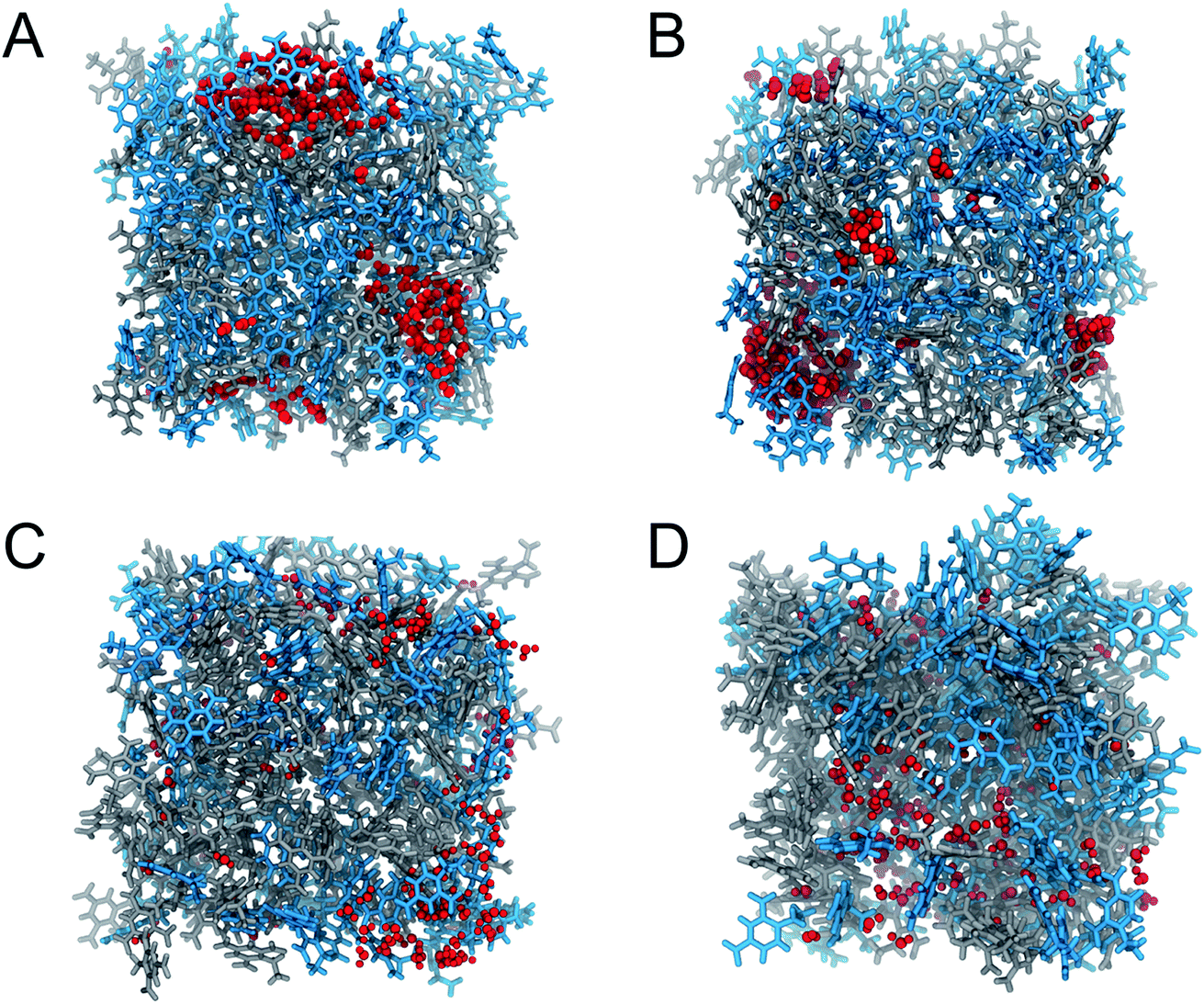Fig. 4 Representations of (A) K10 and water at 298 K, (B) K10 and water at 338 K, (C) R8002 and water at 298 K and (D) R8002 and water at 338 K at the end of MD production runs. In all representations 2,4-DNEB molecules are displayed in blue, 2,4,6-TNEB molecules in grey and water molecules in red.

3.3 Factors affecting the calculation of diffusion coeffcients

The effects of system size, density and method of calculation on the estimation of the diffusion coefficients have been discussed in the literature.^52,54,56 In the work by Wang and Hou, discussed in Section 3.2, MD simulations of water using different box sizes showed that system size influenced the calculation of the self-diffusion coefficients. For that reason, the authors had chosen simulation boxes of at least 30 ų for the calculation of D for aqueous and organic solvents and small organic solutes. In our work, a box size of 40 ų was used in all simulations to predict D, which in view of this earlier work by Wang and Hou was deemed large enough to avoid size effects in the calculations of the diffusion coefficients. However, the results may still have been susceptible to the box size and the number of molecules to some degree.

The sensitivity of the calculated diffusion coefficients to small changes in density has also been reported in the literature and is evident in this study as well.⁵⁶ The self-diffusion coefficient of 2,4,6-TNEB, calculated using both the EE and GK methods, is at least one order of magnitude lower than 2,4-DNEB, despite the structural similarity of the molecules, i.e. the calculated self-diffusion coefficients are particularly sensitive to the difference in density of the two compounds. The same behaviour is repeated for the diffusion of SPC/E water at 298 K, where a much lower diffusion coefficient was obtained for the 2,4,6-TNEB system compared to 2,4-DNEB. The MSD vs. time graphs used to calculate D by the EE formula illustrate these differences and are included in the ESI.† The diffusion coefficients were calculated using the centre-of-mass in the EE and GK methods, which may have affected D due to some flexibility in the 2,4,6-TNEB and 2,4-DNEB molecules. This factor is likely to have been less influential in the calculation of D for SPC/E water in the systems, as this is a rigid water model. Although these factors may have contributed some error to the calculation of D, comparison of the diffusion coefficients obtained via both the GK formula and Einstein equation reinforces the reliability of the results.

4. Conclusion

A classical all-atom force field has been parameterized for 2,4,6-trinitroethylbenzene (2,4,6-TNEB) and 2,4-dinitroethylbenzene (2,4-DNEB). An iterative adjustment of the Lennard-Jones parameters reproduced experimental densities and the force field accurately describes the density of each construct, with 2,4,6-TNEB, 2,4-DNEB, R8002 and K10 within 0.9%, 1%, 1.7% and 1.8% of experimental densities, respectively. The simulated densities of 2,4-DNEB and 2,4,6-TNEB are significantly closer to the experimental values compared to those obtained using a generic force field. Although some of the bond lengths in the MD simulations of 2,4,6-TNEB and 2,4-DNEB are slightly longer than the experimental values, the resulting overestimations of the system volumes in the density calculation are minimal and within reasonable errors. The self-diffusion coefficients of 2,4-DNEB and 2,4,6-TNEB in the pure systems and the diffusion coefficients of the same molecules in the K10 (65% 2,4-DNEB and 35% 2,4,6-TNEB) and R8002 (50% 2,4,6-TNEB and 50% 2,4-DNEB) mixtures were calculated from MD simulations at 298 K using both the Einstein equation and Green–Kubo formula. The self-diffusion coefficient of 2,4-DNEB was greater than 2,4,6-TNEB, which is likely to be due to the lower molecular weight of 2,4-DNEB and the lower simulated density compared to 2,4,6-TNEB, thereby enabling the 2,4-DNEB molecules to move more quickly and with less restriction. Both 2,4-DNEB and 2,4,6-TNEB diffused more quickly through the K10 mixture compared to R8002, as would be expected from the lower simulated density of K10.

The force field was further used in MD simulations to obtain diffusion coefficients, using both the Einstein equation and Green–Kubo formula, for water in 2,4,6-TNEB and 2,4-DNEB and in the energetic plasticiser mixtures K10 and R8002. The diffusion coefficients for water in 2,4-DNEB were faster compared to those for water in 2,4,6-TNEB at both 298 K and 338 K. This suggests that water molecules diffuse more easily if the density of the system is lower, as is the case for 2,4-DNEB compared to 2,4,6-TNEB, probably due to increased space between the molecules. There is no trend in water diffusion rates in the plasticizer mixtures K10 and R8002; water diffusion is marginally faster in K10 compared to R8002 at 298 K, but the opposite was found at 338 K. There is a difference in the distribution of the water molecules in R8002 compared to K10, with the water molecules in R8002 being rather more evenly distributed, with the formation of smaller clusters of and a greater number of isolated water molecules, compared to K10 at both temperatures.

The force field reproduced the densities of 2,4-DNEB, 2,4,6-TNEB and the energetic plasticizers K10 and R8002 to a high level of accuracy. In future, it could be used effectively to investigate the properties of nitrocellulose-based propellants, provided interactions that are not present in either 2,4-DNEB or 2,4,6-TNEB are added and specifically optimized.

Conflicts of interest

There are no conflicts of interest to declare.

Acknowledgements

This research was funded by the Engineering and Physical Sciences Research Council (EPSRC) and The Atomic Weapons Establishment (AWE). The authors acknowledge the use of the UCL Legion High Performance Computing Facility (Legion@UCL), and associated support services, in the completion of this work. NHdL acknowledges AWE for a William Penney Fellowship.

References

1. M. A. Hassan, Effect of Malonyl Malonanilide Dimers on the Thermal Stability of Nitrocellulose, J. Hazard. Mater., 2001, 88, 33–49.
2. B. Zhao, Facts and Lessons Related to the Explosion Accident in Tianjin Port, China, Nat. Hazards, 2016, 84(1), 707–713,  DOI:10.1007/s11069-016-2403-0.
3. P. Seel. Process of Dehydrating Nitrocellulose and Reducing the Fire Risk Thereof, US. Pat., 1398911, 1921.
4. Handbook of Formulating Dermal Applications: A Definitve Practical Guide, ed. N. Dayan, John Wiley and Sons, Inc., Hoboken, HJ, USA, 2016.
5. Dow Wolff Cellulosics, Nitrocellulose Essential for an Extra-Special Finish, Bomlitz, Germany, 1998.
6. G. C. Hale and N. J. Dover, Propellant Powder, US. Pat., 1963992, 1934.
7. A. Garvey and D. W. Price, Energetic Plasticizer Evaluation in Cast-Cured Polymer Based Explosives (PBXs), 2014.
8. P. Arthur, Energetic Polymers and Plasticisers for Explosive Formulations, Melbourne, 2000.
9. T. L. Jensen, J. F. Moxnes, E. Unneberg and O. Dullum, Calculation of Decomposition Products from Components of Gunpowder by Using ReaxFF Reactive Force Field Molecular Dynamics and Thermodynamic Calculations of Equilibrium Composition, Propellants, Explos., Pyrotech., 2014, 39(6), 830–837,  DOI:10.1002/prep.201300198.
10. X. Ma, W. Zhu, J. Xiao and H. Xiao, Molecular Dynamics Study of the Structure and Performance of Simple and Double Bases Propellants, J. Hazard. Mater., 2008, 156, 201–207,  DOI:10.1016/j.jhazmat.2007.12.068.
11. J. Yang, X. Gong and G. Wang, Theoretical Studies on the Plasticizing Effect of DIANP on NC with Various Esterification Degrees, Comput. Mater. Sci., 2014, 95, 129–135,  DOI:10.1016/j.commatsci.2014.07.024.
12. W. Zhu, J. Xiao, W. Zhu and H. Xiao, Molecular Dynamics Simulations of RDX and RDX-Based Plastic-Bonded Explosives, J. Hazard. Mater., 2009, 164(2–3), 1082–1088,  DOI:10.1016/j.jhazmat.2008.09.021.
13. W. Zhu, X. Wang, J. Xiao, W. Zhu, H. Sun and H. Xiao, Molecular Dynamics Simulations of AP/HMX Composite with a Modified Force Field, J. Hazard. Mater., 2009, 167, 810–816,  DOI:10.1016/j.jhazmat.2009.01.052.
14. R. H. C. Janssen, D. N. Theodorou, S. Raptis and M. G. Papadopoulos, Molecular Simulation of Static Hyper-Rayleigh Scattering: A Calculation of the Depolarization Ratio and the Local Fields for Liquid Nitrobenzene, J. Chem. Phys., 1999, 111(21), 9711,  DOI:10.1063/1.480305.
15. J. B. Klauda and B. R. Brooks, CHARMM Force Field Parameters for Nitroalkanes and Nitroarenes, J. Chem. Theory Comput., 2008, 4, 107–115,  DOI:10.1021/ct700191v.
16. D. Michael and I. Benjamin, Molecular Dynamics Simulation of the Water|Nitrobenzene Interface, J. Electroanal. Chem., 1998, 450(2), 335–345,  DOI:10.1016/S0022-0728(97)00653-0.
17. M. L. P. Price, D. Ostrovsky and W. L. Jorgensen, Gas-Phase and Liquid-State Properties of Esters, Nitriles, and Nitro Compounds with the OPLS-AA Force Field, J. Comput. Chem., 2001, 22(13), 1340–1352,  DOI:10.1002/jcc.1092.
18. S. Neyertz, D. Mathieu, S. Khanniche and D. Brown, An Empirically Optimized Classical Force-Field for Molecular Simulations of 2,4,6-Trinitrotoluene (TNT) and 2,4-Dinitrotoluene (DNT), J. Phys. Chem. A, 2012, 116, 8374–8381,  DOI:10.1021/jp305362n.
19. G. Fu, J. Wang and M. Yan, Anatomy of Tianjin Port Fire and Explosion: Process and Causes, Process Saf. Prog., 2016, 35(3), 216–220,  DOI:10.1002/prs.
20. D. A. Case and V. Babin, et al., Amber 14, University of California, San Francisco, 2015.
21. A. Nash, T. Collier, H. Birch and N. De Leeuw, ForceGen: Atomic Covalent Bond Value Derivation for Gromacs, J. Mol. Model., 2017, 24(5), 1–11,  DOI:10.1007/s00894-017-3530-6.
22. J. M. Seminario, Calculation of Intramolecular Force Fields from Second-Derivative Tensors, Int. J. Quantum Chem. Quantum Chem. Symp., 1996, 30, 1271–1277,  DOI:10.1002/(SICI)1097-461X(1996)60:7<1271::AID-QUA8>3.0.CO;2-W.
23. J. Wang, R. M. Wolf, J. W. Caldwell, P. A. Kollman and D. A. Case, Development and Testing of a General Amber Force Field, J. Comput. Chem., 2004, 25, 1157–1174.
24. C. D. Smith, M. Carson, M. van der Woerd, J. Chen, H. Ischiropoulos and J. S. Beckman, Crystal Structure of Peroxynitrite-Modified Bovine Cu, Zn Superoxide Dismutase, Arch. Biochem. Biophys., 1992, 299(2), 350–355,  DOI:10.1016/0003-9861(92)90286-6.
25. S. N. Savvides, M. Scheiwein, C. C. Böhme, G. E. Arteel, P. Andrew Karplus, K. Becker and R. Heiner Schirmer, Crystal Structure of the Antioxidant Enzyme Glutathione Reductase Inactivated by Peroxynitrite, J. Biol. Chem., 2002, 277(4), 2779–2784,  DOI:10.1074/jbc.M108190200.
26. Y.-C. Myung and S.-H. Han, Force Field Parameters for 3-Nitrotyrosine and 6-Nitrotryptophan, Bull. Korean Chem. Soc., 2010, 31(9), 2581–2587,  DOI:10.5012/bkcs.2010.31.9.2581.
27. A. R. Leach. Leach - Molecular Modelling. Principles and Applications 2001, 2nd edn, Pearson Education, Harlow, 2001.
28. J. A. Wickham and R. L. Dilworth, Military Explosives, Washington D. C., 1984.
29. U. C. Singh and P. A. Kollman, An Approach to Computing Electrostatic Charges for Molecules, J. Comput. Chem., 1984, 5(2), 129–145,  DOI:10.1002/jcc.540050204.
30. F.-Y. Dupradeau, A. Pigache, T. Zaffran, C. Savineau, R. Lelong, N. Grivel, D. Lelong, W. Rosanski and P. Cieplak, The R.E.D. Tools: Advances in RESP and ESP Charge Derivation and Force Field Library Building, Phys. Chem. Chem. Phys., 2010, 12(28), 7821–7839,  10.1039/c0cp00111b.
31. E. Vanquelef, S. Simon, G. Marquant, E. Garcia, G. Klimerak, J. C. Delepine, P. Cieplak and F. Y. Dupradeau, R.E.D. Server: A Web Service for Deriving RESP and ESP Charges and Building Force Field Libraries for New Molecules and Molecular Fragments, Nucleic Acids Res., 2011, 39(2), 511–517,  DOI:10.1093/nar/gkr288.
32. P. Cieplak, W. D. Cornell and P. A. Kollman, A Well-Behaved Electrostatic Potential Based Method Using Charge Restraints for Deriving Atomic Charges: The RESP Model, J. Phys. Chem., 1993, 97, 10269–10280.
33. M. J. Frisch and G. W. Trucks, et al., Gaussian'09, Gaussian, Inc., Wallingford CT, 2009.
34. I. Bar and J. Bernstein, The Po -Molecular Complexes Trans-Azobenzene-(Sym-Trinitrobenzene)₂ and N-Benzylideneaniline-(Sym-Trinitrobenzene)₂, Acta Crystallogr., Sect. B: Struct. Sci., 1981, 37, 569–575.
35. D. S. Yufit, The Low-Melting Compounds 1,4-Diethyl-, 1,2-Diethyl- and Ethylbenzene, Acta Crystallogr., Sect. C: Cryst. Struct. Commun., 2013, 69(3), 273–276,  DOI:10.1107/S0108270113003041.
36. I. Bar and J. Bernstein, The Pi-Molecular Complex Stilbene-(Sym-Trinitrobenzene)₂, Acta Crystallogr., Sect. B: Struct. Sci., 1978, 34, 3438–3441.
37. C. S. Choi and J. E. Abel, The Crystal Structure of 1,3,5-Trinitrobenzene by Neutron Diffraction, Acta Crystallogr., Sect. B: Struct. Sci., 1972, 28, 193–201.
38. AWE, Personal Communication, 2016.
39. F. Pristera, M. Halik, A. Castelli and W. Fredericks, Analysis of Explosives Using Infrared Spectroscopy, Anal. Chem., 1960, 32(4), 495–508,  DOI:10.1021/ac60160a013.
40. R. Hollands and V. Fung, High Performance Polymer-Bonded Explosive Containing PolyNIMMO for Metal Accelerating Applications, 2004.
41. J. P. Ryckaert, G. Ciccotti and H. J. C. Berendsen, Numerical Integration of the Cartesian Equations of Motion of a System with Constraints: Molecular Dynamics of N-Alkanes, J. Comput. Phys., 1977, 23(3), 327–341,  DOI:10.1016/0021-9991(77)90098-5.
42. L. Verlet, Computer “Experiments” on Classical Fluids. I. Thermodynamical Properties of Lennard-Jones Molecules, Phys. Rev., 1967, 159(1), 98–103,  DOI:10.1103/PhysRev.159.98.
43. H. J. C. Berendsen, J. P. M. Postma, W. F. van Gunsteren, A. DiNola and J. R. Haak, Molecular Dynamics with Coupling to an External Bath, J. Chem. Phys., 1984, 81(8), 3684–3690,  DOI:10.1063/1.448118.
44. H. C. Andersen, Molecular Dynamics Simulations at Constant Pressure And/or Temperature, J. Chem. Phys., 1980, 72, 2384,  DOI:10.1063/1.439486.
45. R. M. Vrcelj, J. N. Sherwood, A. R. Kennedy, H. G. Gallagher and T. Gelbrich, Polymorphism in 2-4-6 Trinitrotoluene, Cryst. Growth Des., 2003, 3(6), 1027–1032,  DOI:10.1021/cg0340704.
46. J. Hanson, P. B. Hitchcock and H. Saberi, Steric Factors in the Preparation of Nitrostilbenes, J. Chem. Res., 2004, 667–669.
47. C. Steffen, K. Thomas, U. Huniar, A. Hellweg, O. Rubner and A. Schroer, Packmol: A Package for Building Initial Configurations for Molecular Dynamics Simulations, J. Comput. Chem., 2008, 31(16), 2967–2970,  DOI:10.1002/jcc.
48. H. J. C. Berendsen, J. R. Grigera and T. P. Straatsma, The Missing Term in Effective Pair Potentials, J. Phys. Chem., 1987, 91(24), 6269–6271,  DOI:10.1021/j100308a038.
49. J. E. Basconi and M. R. Shirts, Effects of Temperature Control Algorithms on Transport Properties and Kinetics in Molecular Dynamics Simulations, J. Chem. Theory Comput., 2013, 9, 2887–2899,  DOI:10.1021/ct400109a.
50. F. Muller Plathe, Permeation of Polymers a Computational Approach, Acta Polym., 1994, 45(4), 259–293,  DOI:10.1002/actp.1994.010450401.
51. D. R. Roe and T. E. Cheatham, “PTRAJ and CPPTRAJ: Software for Processing and Analysis of Molecular Dynamics Trajectory Data.”, J. Chem. Theory Comput., 2013, 9(7), 3084–3095.
52. D. V. Zlenko, Computing the Self-Diffusion Coefficient for TIP4P Water, Biophysics, 2012, 57(2), 127–132,  DOI:10.1134/S0006350912020273.
53. A. D. Kirk, The Range of Validity of Graham'S Law, J. Chem. Educ., 1967, 44(12), 745–750.
54. J. Wang and T. Hou, Application of Molecular Dynamics Simulations in Molecular Property Prediction II: Diffusion Coefficient, J. Comput. Chem., 2011, 3505–3519,  DOI:10.1002/jcc.21939.
55. A. D. Kulkarni, K. Babu, S. R. Gadre and L. J. Bartolotti, Exploring Hydration Patterns of Aldehydes and Amides: Ab Initio Investigations, J. Phys. Chem. A, 2004, 108(13), 2492–2498,  DOI:10.1021/jp0368886.
56. T. Fox and P. A. Kollman, Application of the RESP Methodology in the Parametrization of Organic Solvents, J. Phys. Chem. B, 1998, 102(41), 8070–8079,  DOI:10.1021/Jp9717655.

---

Footnote

† Electronic supplementary information (ESI) available. See DOI: 10.1039/c7ra12254c

---