Solvent effects on the excited state characteristics of adenine–thymine base pairs

Abstract

The ability to dissipate electronic excitation and thus prevent photo-induced damage and provide natural protection and photo-stability is, perhaps, the most significant characteristic of DNA bases as the building blocks of life on Earth. Therefore, it is understandable that studies of the excited states of DNA bases have attracted remarkable research interest. The challenge of experimental studies of DNA photo-physics stems from the intrinsic complexity of the dynamical behaviours of the excited states. In this regard, quantum mechanical methods for studying excited electronic states provide helpful insight. In this study we utilize time dependent density functional theory (TDDFT) to analyse the excited states of the DNA base-pair adenine–thymine in both the canonical Watson–Crick and stacked configurations. The excited state wavefunctions are analysed and visualized in terms of the one-electron transition density matrix (1TDM) and natural transition orbitals. The environmental effect on the excited states is considered by using a non-empirical effective fragment potential method. The extent of de-localization and the charge transfer character of the excited states in the near- and far-ultraviolet region of the electromagnetic spectrum are identified. It is also shown that the environmental effect on the de-localization is significant and varies with the configuration. Additionally, localized Frenkel type states, as well as de-localized states involving multiple molecular fragments, are also identified.

---

1 Introduction

The major cause of damage to the genetic code and, eventually, processes that lead to mutagenesis, carcinogenesis and apoptosis, can be identified as a cascade of photochemical processes that are triggered by the strong absorption of ultraviolet (UV) light by DNA. The other factors that may induce DNA damage include ionizing radiation and reactive chemical species such as genotoxic chemicals and free radicals.¹ Oxidative damage of DNA is the result of direct interaction with ionizing radiation or with free radicals and reactive oxygen species that are induced by UV radiation.² The reactivity of DNA bases in their excited states is consequently of the utmost importance. Despite the strong absorption of UV light, DNA bases were naturally selected as the building blocks of life because of the high photo-stability of the isolated nucleobases. It is now well established that the photo-stability of these molecules stems from the existence of efficient non-radiative relaxation mechanisms^1,3 that support ultra-fast (few ps) decay from the lowest excited singlet states to the electronic ground states. However, long-living excited states are found in DNA strands, particularly in stacked domains.^4,5 A study using picosecond time-resolved infrared spectroscopy found that the single-stranded cytosine polymer has a longer excited state lifetime than that of the monomer, due to nearest neighbour interactions.⁶ Such base–base interactions, which lead to longer lived excited states, are more prone to excited state damage. These excited states are charge-separated states and the charges are delocalized in the stacked domains.⁵ The delocalization of charges over a few bases and decay by charge recombination to the neutral ground state on the 100 ps time scale may have biological implications for photo-mutation and localisation of damage.

Therefore studies of the excited states of DNA bases in their various configurations and, in particular, determination of the extent of de-localization and its temporal changes, are fundamental for understanding the photo-stability of the DNA molecule.⁷

The photo-stability of nucleobases leading to the mechanism of self-protection from UV-damage is further enhanced by the interactions in their excited states through inter-strand hydrogen bonding and intra-strand stacking.^8–10 These inter- and intra-strand interactions lead to different excited state dynamics than those of the isolated DNA bases. Experimental studies¹¹ utilizing structurally sensitive transient IR spectroscopy have shown how base–base interactions lead to extended-lifetime electronic excited states of the nucleic acid bases. In general, the close proximity of multiple chromophores can trigger the formation of a combination of excited states. Consequently, the excited states of a DNA molecule are expected to be dependent on the sequence as well as on the relative positions of the nucleobases. Experimental studies utilizing time-resolved spectroscopy also support the existence of different excited state dynamics of bases with stacking interactions, in contrast with the dynamics of isolated DNA bases.^12,13 The nature of these interactions and their effect on the characteristics of the excited states are still not fully understood. In order to interpret experimental spectra, a deep understanding of how intra-strand excimer formation is linked to charge-transfer (CT) character is essential. Furthermore, the role of de-localized excitons cannot be ignored.¹⁰

In this regard, a number of issues are still open for discussion, including (i) a detailed characterization of the excited states during the UV absorption process, (ii) the degree of de-localization, (iii) the effect of the solvent on the nature of an excited state, (iv) the CT effect on the excited state dynamics and (v) the role of dark states.

The excited states of an adenine (A):thymine (T) system in two different arrangements, canonical Watson–Crick hydrogen bonded (AT-WC) and stacked (AT-S), are investigated in this study. Research on the de-localization of the excited states of multiple chromophores (exciton states) in DNA can be traced back to the 1960s.^14,15 Experimental and theoretical investigations have, however, only been carried out over the past few decades.¹⁶ In particular, recent advances in ultra-fast time resolved technologies have helped to provide insight into photo-induced dynamic processes¹⁷ as well as information about the structural modifications that occur during the rapid processes associated with deactivation of the photo-induced excited states.¹⁸

Nonetheless, there are still some limitations to both experimental and theoretical methods. Experimentally, it is relatively easy to prepare samples and carry out experiments on single-stranded poly-DNA base systems. In contrast, the effect of H-bonding, separate from the effect of stacking interactions, could not be studied until recently due to the instability of a single Watson–Crick pair in solution. Authors of recent studies, however, were able to stabilize individual guanine–cytosine (GC)¹⁹ and AT²⁰ Watson–Crick base pairs in chloroform and study the involvement of electron driven proton transfer (EDPT) in the deactivation dynamics, excluding any possible participation of excimer states induced by π-stacking. Moreover, the fast decay of excited states and the limited resolution of experimental techniques mean that measuring properties, which can be connected to the calculated extent of de-localization of the excited state, is very complicated.²¹ Therefore, theoretical simulations provide a complimentary set of tools for modelling the properties of complicated molecular configurations and help explain the features of experimental spectra (see, e.g., ref. 22).

Despite advances in the development of quantum mechanical (QM) methods, as well as increased computational power, studying the excited electronic states of DNA bases remains challenging.²³ Recent methodological and computational advances have played an important role in clarifying the mechanisms of photo-stability of DNA bases.²⁴ Advances in computational methods and hardware enable simulations of the excited state behaviours of molecular systems containing up to 100–150 atoms, with fairly good accuracy observed. Continuous advances in methods and computational power have also allowed the tackling of a direct simulation of photo-induced non-adiabatic dynamics in nucleobases and small DNA fragments, thus providing a fundamental tool for studying photo-activated dynamics in DNA.^1,25

Numerous theoretical studies have been carried out in recent years on DNA base systems composed of different configurations and at various levels of theoretical modelling. A comprehensive review on these studies was published recently.²⁴ High-level multi-reference methods such as complete active space self-consistent field, CAS with perturbation theory to second order (CASPT2), and multi-reference configuration interaction have been used^26–30 to study the excited states of single nucleobases. The approximate coupled cluster singles-and-doubles method CC2 (ref. 31) has also been used to study the excited states of single nucleobases. However, the extensive use of such highly correlated methods for systems beyond single bases is computationally prohibitive. Ab initio methods at the CASSCF/3-21G level of theory and mixed quantum/classical (QM/MM) molecular dynamics simulations have been used to study the detailed structural and dynamical characteristics of the ultrafast radiationless deactivation mechanism of a photo-excited C–G base pair in the gas phase and embedded in DNA.³² Currently, the highest level theoretical methods used for excited state calculations of stacked dimers and Watson–Crick pairs are EOM-CCSD and EOM-CCSD(T).^33,34 A natural choice for theoretical modelling of the excited states of large systems is time dependent density functional theory (TDDFT), due to its computational efficiency and accuracy, subject to the choice of functional. A recent benchmark study of two stacked dimers, adenine–thymine (AT) and guanine–cytosine (GC), has been carried out using a number of density functionals to elucidate the local excitation and charge-transfer (CT) characteristics.³⁵

Clear evidence of the importance of solvent effects on the excited state processes of DNA bases has been found experimentally. The role of environmental effects leading to significant changes in the orbital energies of DNA is discussed in ref. 36. Moreover, it was shown that solvent effects influence the relative energy of the charge transfer state (CT) with respect to the bright state.³⁷ Previous studies on the excited states of nucleobases have addressed the effect of solvent on the excited state characteristics with some approximations. The approximate methods used were limited to either QM/MM models, where the solvent effects are considered with molecular mechanics (MM) models,³⁸ or polarization continuum models.^35,39 An explicit solvent model was also included in a QM calculation.⁴⁰ The number of explicit water molecules included in this model was extremely limited and their relative positions were selected arbitrarily. Some molecular dynamics studies were also carried out in order to fulfil the sampling requirements.^40–44 In this study we use an effective fragment potential (EFP) based model to include the effect of solvent on the excited state properties. EFP is effectively a quantum mechanical based potential that requires no empirical parameters to build the polarizable force field.⁴⁵ Furthermore, in contrast to the standard QM/MM model, the excited state implementation of EFP includes the polarization responses of the environment to the excited state properties.

The vast majority of quantum mechanical studies of the electronic excitations of many-particle molecular systems are usually limited to computing the electronic excitation energies and oscillator strengths of the molecular systems based on ab initio methods (e.g. ADC, CC or EOM-CCSD) or time-dependent linear response density functional theory (TDDFT). However, a significant amount of information on the excited state characteristics can be obtained by analysing the wavefunctions. Conventional descriptions of excited states wavefunctions involve analysing the response vectors of the excited states in terms of the ground-state molecular orbitals. The ground state occupied (hole) and virtual (particle) orbitals of small molecules involved in an excitation are considered separately. The excited states are then defined based on the shapes of these orbitals and are consequently classified according to their character, e.g. nπ* or ππ*. For large molecular systems the description of an excited state might involve contributions from many ground-state molecular orbitals, thus making analysis very complicated. Furthermore, some properties of interest may not be directly deduced from the shapes of the orbitals at all and may require decisive information that lies in the phases of their superpositions. For example, in the case of dimers only a sign change differentiates between the charge resonance and excitonic states.^38,46 For multimers the situation becomes even more intricate.

Despite extensive research on DNA bases and their various configurations, a comprehensive analysis of the excited state wavefunctions of base pairs, and particularly the effect of solvent on the excited state characteristics, is still missing. In this study, we utilize wavefunction-based analysis to study the excited state characteristics of AT base pairs, where the orbital representation of the excited state is replaced by a representation of a correlated electron–hole wavefunction. The central idea is to move away from the molecular-orbital picture to the quasi-particle exciton representation. Such a quasi-particle exciton representation can be constructed in a quantum-chemical context by using a one-particle transition density matrix (1TDM) representing the transition between the ground and excited-state wavefunctions.^47,48 Recently, a one-particle transition density matrix (1TDM) based tool, for analysis of charge resonance and excitonic correlation phenomena in quantum chemical calculations, has demonstrated significant potential in this field.^49,50 The aim of this study is to provide a more accurate description of excited states, thus giving more insight into the photo-induced charge transfer and de-localization problem.

2 Methods and computational details

A reliable theoretical prediction of the electronic spectra and excited state properties of large molecular complexes demands the right balance of accuracy and tractability in terms of computational resources. In this regard, time-dependent density functional theory (TDDFT) turns out to be one of the most efficient tools developed so far. TDDFT predicts the excitation energies for the low lying excited states of some cases with good accuracy.^51–53 However, TDDFT with conventional DFT functionals yields severely underestimated excitation energies^54,55 for electronic excitations with charge transfer characteristics, or polarizabilities in conjugated systems.⁵⁶ The primary limitation of conventional DFT functionals stems from their inability to address the correct asymptotic behaviour of the exchange–correlation potential that is sensitive to long distance orbital–orbital interactions. Hybrid GGA functionals such as B3LYP and PBE0 improve the asymptotic behaviour of the exchange–correlation potential but still fall short of predicting the correct charge transfer states. Consequently, a series of long-range corrected (LRC) density functionals has been developed^57,58 which exhibit the correct asymptotic behaviour and improve the description of the Rydberg and charge transfer excited states. In particular, the family of ωB97 functionals developed by Head-Gordon and co-workers⁵⁹ demonstrates overall excellent performance in the prediction of long-range charge-transfer excitations. A recent application of the ωB97X functional to compute the electronic spectra of photo-active organometallic complexes showed a very good agreement with the available experimental results.⁶⁰ Therefore, in the present research the LRC DFT functional ωB97X along with the Dunning’s correlation consistent basis sets of cc-pVTZ⁶¹ were used.

Although significant progress has been achieved in the explicit treatment of vibrational effects in theoretical electronic spectra,^62,63 these applications demand a careful assessment of the affordability of the computational cost for medium-to-large molecules. In our case, the protocol for a simulation process that accounts for the explicit vibrational effects along with reliable solvent effects had not yet been developed. Therefore, the theoretical band shapes of the TDDFT electronic spectra were generated by approximating the vibrational effects in terms of Gaussian convolution techniques. For each electronic transition a Gaussian function was assigned, where the amplitude of each Gaussian was equal to the value of the oscillator strength of the transition. The Gaussian FWHM was set to 0.5 eV. The final convolved band shape was created by summing all of the Gaussians for each particular energy value.

The reference geometries of the AT base pair in the stacked and canonical Watson–Crick configurations were taken from a benchmark data set of JSCH-2005.⁶⁴ The geometries of the complexes considered were calculated from the ground state of the B-DNA structure and optimized at the RI-MP2 level by using the TZVPP basis set.⁶⁵

The effects of solvent on the electronic spectra were treated by using one of the most sophisticated approaches, the effective fragment potential (EFP) method.⁶⁶ Gordon and co-workers developed the EFP method where each solvent molecule is represented by an effective fragment (EF). A parameter set for each unique type of solvent is determined from a preparatory ab initio calculation without fitting to any empirically determined parameters. This parameter set, consisting of distributed multipoles and polarizability tensors, is then used to create a polarizable model potential. The advantage of the EFP method stems from the fact that the method includes self-consistent polarizability, which allows the solvent to respond to the changing electron density of the solute upon excitation. Hence, EFP is a viable approach for predicting and interpreting the effects of solvents on the properties of electronically excited states. In this work we surrounded solute base pairs with hundreds of water molecules as effective fragments. The initial geometry of the solute–solvent complex was then optimized by applying a universal force field implemented in IQMol.⁶⁷ The optimized structure of the complex was then used in further TDDFT calculations.

A detailed analysis of the excited states was carried out by applying a scheme based on the one particle transition density matrix (1TDM).⁶⁸ Such an analysis is capable of identifying charge resonance and excitonic correlation effects and, subsequently, quantifying a number of the properties of electron–hole pairs.⁴⁷

Direct interpretation of the excited states by quantum chemical calculations, expressed in terms of the energy and a set of amplitudes which represent the contribution of multiple states, is often difficult. Therefore, in order to obtain a simple orbital interpretation of “what got excited to where”,⁶⁹ natural transition orbitals (NTOs) can be constructed by carrying out a singular value decomposition (SVD)⁷⁰ of the 1TDM.^68,69

However, in the case of large and complex molecular systems with multiple chromophores, several NTO pairs are often needed to describe an excited state. Thus for a quantitative description of the excited states, further analysis of the transition density matrix is needed. A tool for such analysis was recently proposed by Plasser et al.⁴⁷ By applying this analytical procedure, one can assign numerical values to various properties describing the extent of contribution from participating fragments to the excited state, extent of de-localization, and charge transfer characteristics.

The localization of charge during excitation is characterized by the type of electronic transition. When the hole and particle orbitals are on the same fragments, this constituents a Frenkel-type transition. Otherwise, the transition is of a charge-separated type, as the hole and particle orbitals are spread over a number of fragments. Both types can be localized or de-localized, depending on the number of fragments that are contributing to the excitation.

The charge transfer matrix, Ω, obtained from the transition density matrix, is the central quantity of the 1TDM based analysis. In principle, the Ω matrix is obtained by integrating the hole/particle density over all space. For an orthonormal (e.g. MO) basis, Ω is the squared Frobenius norm of the transition density matrix expressed within the MO basis.⁴⁷ For practical purposes, the Ω matrix can be partitioned into contributions from different molecular fragments, thus giving a picture of the electron–hole distribution. In our analysis we defined adenine and thymine of the base pair as fragments 1 and 2, respectively. The quantified parameter, charge transfer number, of such an analysis is given by the elements of the matrix Ω_AB, which is obtained from the 1TDM by using a procedure analogous to that of Mulliken population analysis.⁴⁷ The element of matrix Ω_AB gives the probability of finding the hole on fragment A while the excited electron is on fragment B. An electron–hole pair correlation plot can be constructed by using the magnitudes of these matrix elements to directly visualize the electron–hole pair correlation. The diagonal elements of this matrix correspond to Frenkel-type excitations, while the off-diagonal elements correspond to the contribution of charge separated states to the studied excited state.

Alternatively, from these matrix elements some other quantitative statistical descriptors can be devised that represent charge transfer, de-localization and other excited state characteristics.

In order to identify the charge transfer state, the weight of the charge transfer configurations can be determined³⁸ as the charge transfer character (CT). For a Frankel type excitonic state, this measurement is either 0 or 1 for completely charge-separated transitions.

The extent of de-localization of the excitation over fragments can be formulated by using the concept of a participation ratio (PR) to compute the number of fragments that participate in the excitation. For a state that is localized only on one fragment or a complete charge transfer state between two fragments, PR = 1, otherwise, for de-localized states or charge resonance states PR can be as large as the number of fragments.

The extent of mixing between Frenkel-type and charge-separated states is given by the coherence length (COH). This gives the average electron–hole separation. If the excitation is purely of one type then COH = 1, otherwise, the COH is less than 1. The average position of the exciton is given by a single quantity, POS. POS can take values between 1 and the number of the fragments.

Another important quantity for excited state analysis is the number of how many different NTOs are participating and thus how many transitions are necessary to describe the excited state. This quantity is defined by a value, PR_NTO. In fact, PR_NTO quantifies the number of non-zero singular values (SVs) obtained from the SVDs of the 1TDM. PR_NTO is an intrinsic measure that provides information about electronic resonances and does not require the definition of any fragments.³⁸ In order to obtain all of the aforementioned statistical descriptors from analysis of the 1TDM, TheoDore^47,71 is used.

All of the ab initio calculations were carried out using the Q-Chem⁷² package. The Jmol⁷³ program was used for visualization.

3 Results and discussion

3.1 Electronic spectra

The response vectors of the excited state configurations of the first twenty singlet states were calculated using TDDFT methods with a long range corrected density functional, ωB97X. The orbital energies and oscillator strengths obtained from these calculations were used to construct the electronic spectra of the A–T base pairs. The complete set of data of the vertical electronic excitation energies, oscillator strengths and some statistical descriptors of the AT base pair in both the stacked and WC configurations in the gas phase and in solution (both relaxed and constrained base pair structures) is presented in the ESI.† The computed spectra for both the canonical and stacked configurations are shown in Fig. 1. There are a few generic features of these spectra. First, there is no absorbance in the visible region of the electromagnetic spectrum and the absorbance in the UV region is intense. All configurations have two distinct electronic bands.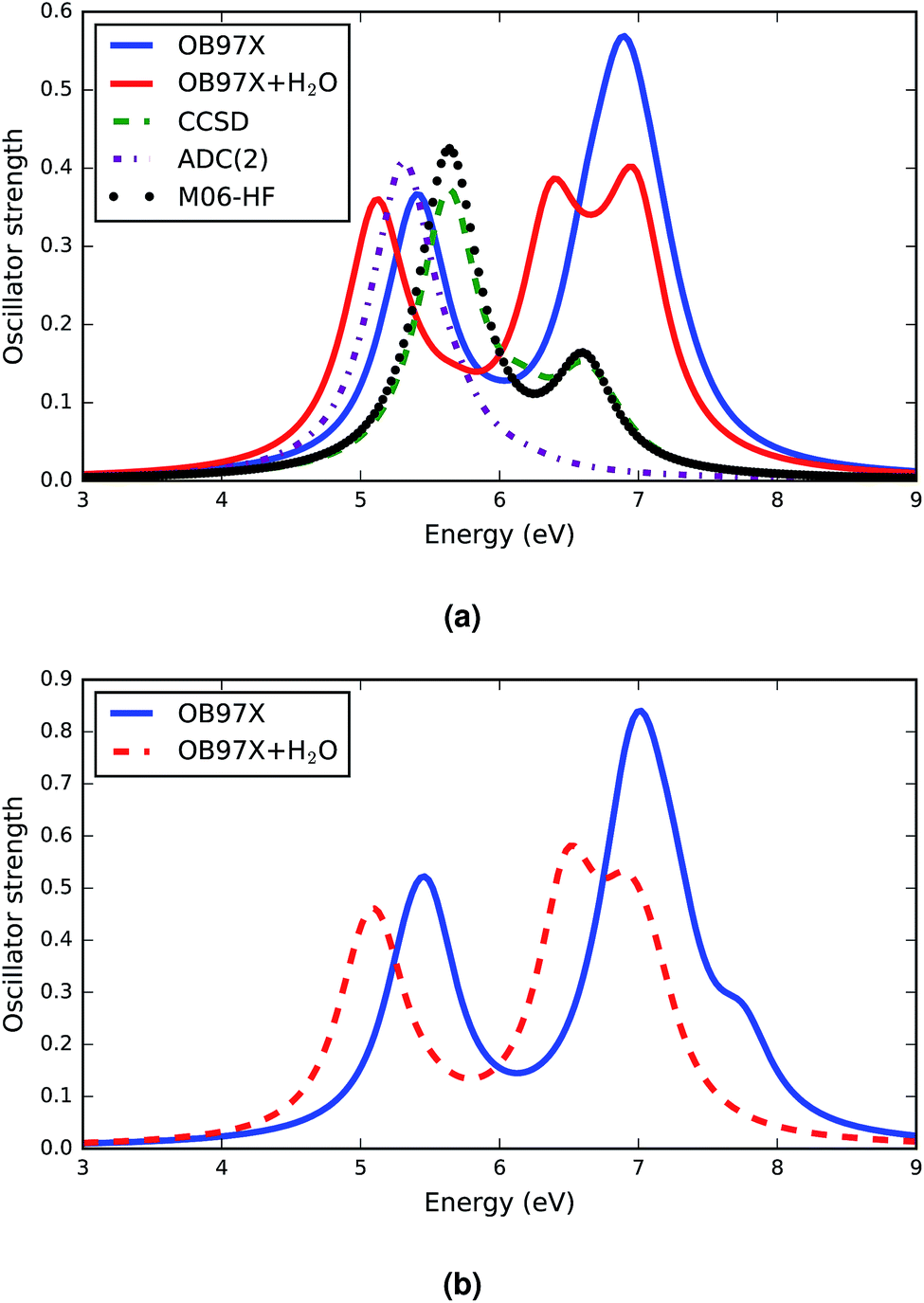

Fig. 1 Simulated absorption spectra of AT-S (a) and AT-WC (b) computed using TDDFT methods with the long range-corrected ωB97X functional. The oscillator strengths are not normalized and the absorption bands are represented by FWHM = 0.5 Gaussians. A comparison of the electronic spectra computed using various ab initio and DFT methods is depicted in (a). The electronic spectra with the solvent effect computed using the TDDFT and EFP formalism are presented by the solid red and dashed red lines.

A comparison of the TDDFT computed electronic spectra of the AT-S configuration with the available spectra from the literature^33,35 is shown in Fig. 1a. The comparison shows that the long range-corrected ωB97X functional qualitatively reproduces the band shape of the spectra. An explicit consideration of the vibrational structures of single electronic transitions⁷⁴ could potentially reproduce a more realistic shape of the band envelopes that usually vary strongly between transitions (broad versus narrow peaks). However, as mentioned above, we used a uniform symmetric Gaussian convolution function instead of explicit vibrational frequency calculations to produce the band envelope in order to keep the computational cost tractable.

The band peak of the AT-S configuration is red shifted and blue shifted by about 0.2 eV from the band peak computed using the CCSD³³ and ADC(2)³⁵ methods, respectively. The amplitude of the absorption band computed using the TDDFT ωB97X functional agrees very well with the results obtained from CCSD calculations. The results of the other DFT functional, M06HF, presented in Fig. 1a, show a very good agreement with the CCSD results for the band shape and band energy, although they overestimate the amplitude. The spectra computed using ab initio methods and DFT functionals cover only the first ten singlet excited states. Our TDDFT computed spectra provide data for the first twenty singlet states in the excitation energy range of the far ultraviolet region. There is a significant absorption band in this energy domain. Detailed analysis shows that there are at least 3 bright transitions in this region. The nature of these transitions is discussed in section 3.4.

The electronic spectra of AT-WC are presented in Fig. 1b. The overall features of the spectra are analogous to those of the AT-S spectra. The AT-WC electronic spectra, composed of the first twenty excited states, also show that there are two distinctive absorption bands; one is in the mid-ultraviolet range and the other is in the far-ultraviolet energy range. Detailed analysis of the electronic spectra of AT-WC along with a quantitative analysis of the excited state based on the natural transition orbital is given in section 3.4.

The effect of solvent on the electronic spectra of the AT base pairs in two different configurations is distinct but analogous for configurational variations. Overall, there is a solvent-induced red shift in the electronic spectra of both the stacked and canonical configurations, as represented by the solid red and dashed red curves in Fig. 1. This kind of red shift is predicted for individual DNA bases when applying different theoretical methods.²⁴

As in the gas phase, the solvated AT base-pairs show two distinct absorption bands within the mid- and far-ultraviolet energy ranges of their respective electronic spectra. However, the solvent effects significantly affect the intensity and broadening of the spectra. The intensities of the absorption bands of both AT-S and AT-WC are lowered by the solvent effects. The solvent effects also broaden the electronic spectra of both AT base-pair configurations, particularly in the far ultraviolet energy range. The other distinguished feature of the solvent effect is the broadening of the spectral line, which is in agreement with previous studies.³⁵ The broadening of the spectra in solution can be attributed to the hydrogen bonding interactions between the solvent molecules and DNA bases.

3.2 Effect of geometry relaxation in solution

The excitation energy spectra in solution obtained in this study exhibit some discrepancies with some of the existing studies in the literature. In particular, our results for the AT-S system do not agree with the results presented in ref. 35. According to the data presented in ref. 35, the nπ* states of AT-S are significantly destabilized when going from the gas phase to water solution. In contrast, our results show a significant stabilization of the nπ* states in water. In ref. 35 the solvation effect on the excited state of the AT stacked configuration was considered in terms of a PCM model. In this study, the solvent effect was accounted for only in terms of bulk electrostatic effects, and does not consider geometry relaxation in solution. There is another study by Dargiewicz et al.³⁷ that looked into the effect of solvent on the AT Watson–Crick base pair. This study also modelled the bulk solvent using the PCM approximation. Moreover, they acknowledged that the presence of explicit solute–solvent hydrogen bonds is very important for the excited states with nπ* character. The effect of geometry relaxation in the presence of solvent molecules is not considered in this study either. On the other hand, our study considers the solvent effect by applying an effective fragment potential where explicit solute–solvent interactions are calculated. The effect of geometry relaxation in solution in our study is included by optimizing the whole cluster geometry (the geometry of the base pair along with the surrounding water molecules) by using a universal forcefield. Therefore, a careful verification of the role of geometry relaxation in solution is needed to clarify the discrepancies between the results in these two studies.

In order to further verify our results, we carried out a series of ab initio ADC(2)/6-31G calculations of the stacked AT system in the gas phase, in water without relaxing the base pair geometry, and in water with optimized geometry. To limit the computational expense we calculated only the first 4 excited states of the system with this computationally expensive method. The results are presented in Table 1 along with the results obtained by applying the ωB97x/cc-pVTZ model for the same structural configurations. Table 1 shows that the nπ* states of the stacked AT system are destabilized in water if the geometry is not relaxed, which agrees with the trend observed in previous PCM calculations.³⁵ However, if the base pair geometry is relaxed in solvent, the nπ* states are stabilized due to dipole interactions. Furthermore, geometry relaxation has a significant influence on other excited state characteristics such as charge transfer states and UV bright states. We assume that the relaxation of the larger stacked or longer DNA strand configurations might not be as significant as that of the dimer stack considered here, because the geometry of large stacked or long DNA strands is already constrained by neighbouring bases and sugar moieties. However, our results show that a mean field type solvent model such as PCM without any consideration of geometry relaxation is not adequate to address the effect of solvent on the excited state characteristics of DNA bases in particular and any stacked configurations in general.

Table 1 Excitation energies (ΔE, eV) and oscillator strengths (f) for the excited states of AT-S in the gas phase (AT), in solution (AT_S) and in solution with the geometry optimized (AT_S(O))

State	ADC(2)/6-31G						ωB97x/cc-pVTZ
	AT		ATS		ATS(O)		AT		ATS		ATS(O)
	ΔE (eV)	f	ΔE (eV)	f	ΔE (eV)	f	ΔE^a (eV)	f	ΔE (eV)	f	ΔE^a (eV)	f
a Transition types are given in parentheses.
S1	4.83	0.00	5.06	0.00	4.45	0.00	5.23 (nπ*)	0.01	5.23	0.042	4.84 (nπ*)	0.00
S2	5.07	0.00	5.29	0.01	4.52	0.00	5.24 (nπ*)	0.04	5.43	0.199	4.96 (ππ*)	0.03
S3	5.28	0.08	5.36	0.07	4.79	0.17	5.40 (ππ*)	0.24	5.48	0.032	5.10 (nπ*)	0.04
S4	5.45	0.03	5.39	0.01	5.19	0.16	5.48 (nπ*)	0.031	5.54	0.05	5.12 (ππ*/nπ*)	0.27
S5							5.52 (ππ*)	0.02	5.69	0.044	5.41 (ππ*)	0.02
S6							5.97 (ππ*)	0.01	5.70	0.005	5.65 (nπ*)	0.00
S7							6.11 (nπ*)	0.00	6.04	0.002	5.69 (ππ*)	0.03
S8							6.40 (nπ*)	0.00	6.4107	0.053	6.17 (nπ*)	0.00
S9							6.62 (nπ*)	0.003	6.51	0.00	6.36 (nπ*/ππ*)	0.06
S10							6.64 (ππ*)	0.002	6.55	0.17	6.37 (ππ*/nπ*)	0.22
S11							6.87 (ππ*)	0.24	6.69	0.216	6.62 (ππ*)	0.03

---

3.3 Frontier molecular orbitals

Frontier molecular orbitals of AT-S and AT-WC both in the gas phase and in an aqueous environment are depicted in Fig. 2 and 3. In both configurations, the electron densities in the Frontier orbitals are mostly localized on one fragment of the base pair. In the gas phase AT-S configuration the major contribution to the HOMO−1 and LUMO is from the nπ orbitals localized on thymine. However, the major contribution to the HOMO and LUMO+1 is from the π and nπ orbitals, respectively, which are localized on the adenine fragment of the base-pair.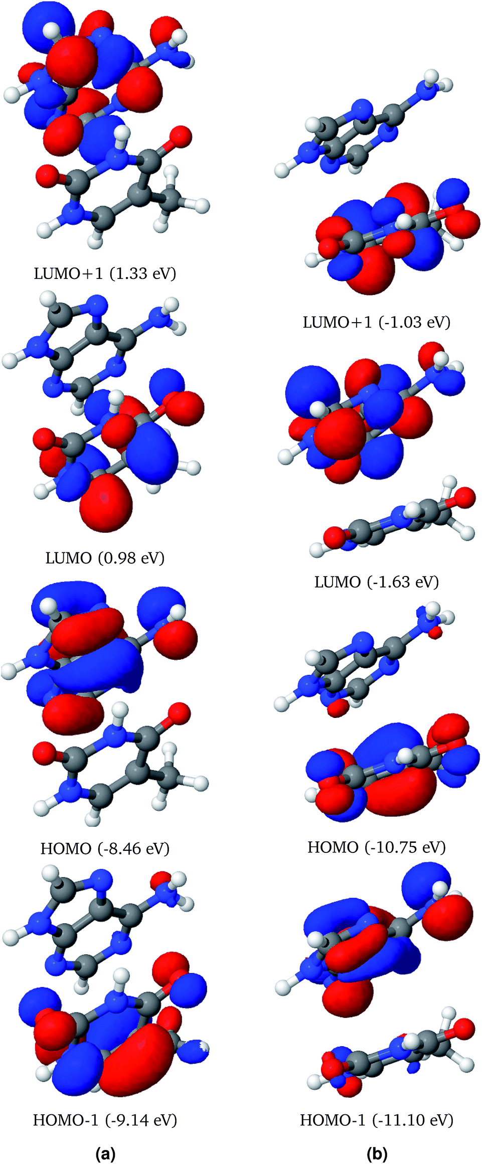

Fig. 2 Three dimensional plots of the representative Frontier molecular orbitals (FMO) of the AT-S system in the gas phase (a) and solvated in a water droplet (b), computed using the ωB97X functional. The orbital energies are given in parentheses.

Fig. 3 Three dimensional plots of the representative Frontier molecular orbitals (FMO) of the AT-WC system in the gas phase (a) and solvated in a water droplet (b), computed using the ωB97X functional. The orbital energies are given in parentheses.

Solvent effects are significant for the Frontier molecular orbitals of AT-S. The solvent effects shift the electron density in the Frontier molecular orbitals from one fragment to the other. For example, the electron density in the HOMO of the AT-S in the aqueous phase is localized on thymine. In contrast, the gas phase electron density of the HOMO is localized on adenine.

Analogous to the AT-S configuration, the electron densities of the HOMO−1 and LUMO are localized on thymine. However, both of these orbitals exhibit π characteristics. Similarly, the electron densities of the HOMO and LUMO+1 are localized on adenine.

Unlike for the AT-S configuration, solvent effects do not shift the electron density localization from one fragment to the other in the AT-WC configurations.

3.4 Analysis based on transition density matrix (1TDM)

AT-S. Characterization of the first eleven singlet excited states of the AT-S configuration in the gas phase can be carried out using the data presented in Table 2. The extent of de-localization was analysed using the quantitative information given by the values of POS and PR in Table 2. The PR values presented in Table 2 show that the singlet state S₁ and the S₄ to S₉ states of AT in the gas phase are highly localized. The PR values of these states do not exceed 1.09. The S₁ and S₉ states are localized on thymine, which is defined as fragment 2. Accordingly, the POS values of these states are close to 2.0. States S₄, S₅, S₇ and S₈ are localized on adenine. The extent of de-localization of the S₂, S₃ and S₁₀ states is given by the PR values 1.37, 1.31 and 1.57, respectively. However, the POS values of these states indicate that the major part of the hole and particle density of the S₂, S₃ and S₁₀ states is on fragments 2, 1 and 1, respectively.

Table 2 Statistical descriptors (e.g. Ω, POS, PR, CT and COH, see the text for details) for the first 11 excited states of AT-S in the gas phase (AT) and in solution (AT_SOL)

State	Ω		POS		PR		CT		COH
	AT	ATSOL	AT	ATSOL	AT	ATSOL	AT	ATSOL	AT	ATSOL
S1	0.83	0.90	1.97	1.02	1.06	1.04	0.06	0.04	1.06	1.04
S2	0.86	0.91	1.84	1.75	1.37	1.61	0.10	0.09	1.14	1.16
S3	0.89	0.84	1.14	1.85	1.31	1.34	0.06	0.10	1.07	1.13
S4	0.86	0.90	1.02	1.32	1.03	1.78	0.03	0.08	1.03	1.15
S5	0.84	0.87	1.04	1.05	1.09	1.11	0.08	0.06	1.09	1.07
S6	0.96	0.92	1.50	1.02	1.08	1.04	0.94	0.04	1.07	1.04
S7	0.84	0.91	1.02	1.48	1.04	1.07	0.04	0.93	1.04	1.07
S8	0.89	0.84	1.02	1.01	1.04	1.02	0.04	0.02	1.04	1.02
S9	0.80	0.69	1.96	1.81	1.08	1.43	0.07	0.09	1.08	1.12
S10	0.78	0.78	1.24	1.33	1.57	1.79	0.18	0.23	1.29	1.47
S11	0.87	0.86	1.73	1.74	1.64	1.64	0.19	0.51	1.34	1.69

---

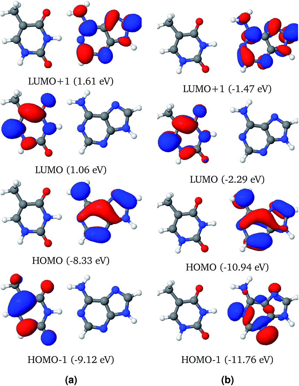
Among the first eleven singlet excited states of the AT-S configuration, one state is identified as the charge transfer state. The CT value in Table 2 convincingly shows that the S₆ state (CT = 0.94) is the charge transfer state. The NTO pair and the electron–hole correlation matrices (Ω matrices) in Fig. 4a show that this is a complete charge transfer state from adenine to thymine. The hole density is localized on the ground state of adenine, whereas the particle density is localized on the excited state of thymine. The value of PR, being close to unity, also indicates that there is no de-localization involved in this charge transfer state. The charge transfer characteristics of the S₆ state, identified by the ωB97x/cc-pVTZ model, agree with earlier calculations.³⁵

Fig. 4 Charge transfer states of AT-S in the gas phase (a) and in solution (b). The symbol above the arrow indicates the singlet excited state that is described by the NTO pairs presented in the figure. The panel to the left of the arrow shows the hole density and the panel to the right of the arrow shows the particle density. The symbol, λ, below the arrow gives the weight of the respective configuration. Electron–hole correlation plots (Ω matrix) of the charge transfer excitation states are presented at the bottom of each figure. The Ω matrix is a 2 × 2 matrix here as the AT dimer is divided into two fragments. Adenine and thymine are defined as fragments 1 and 2, respectively.

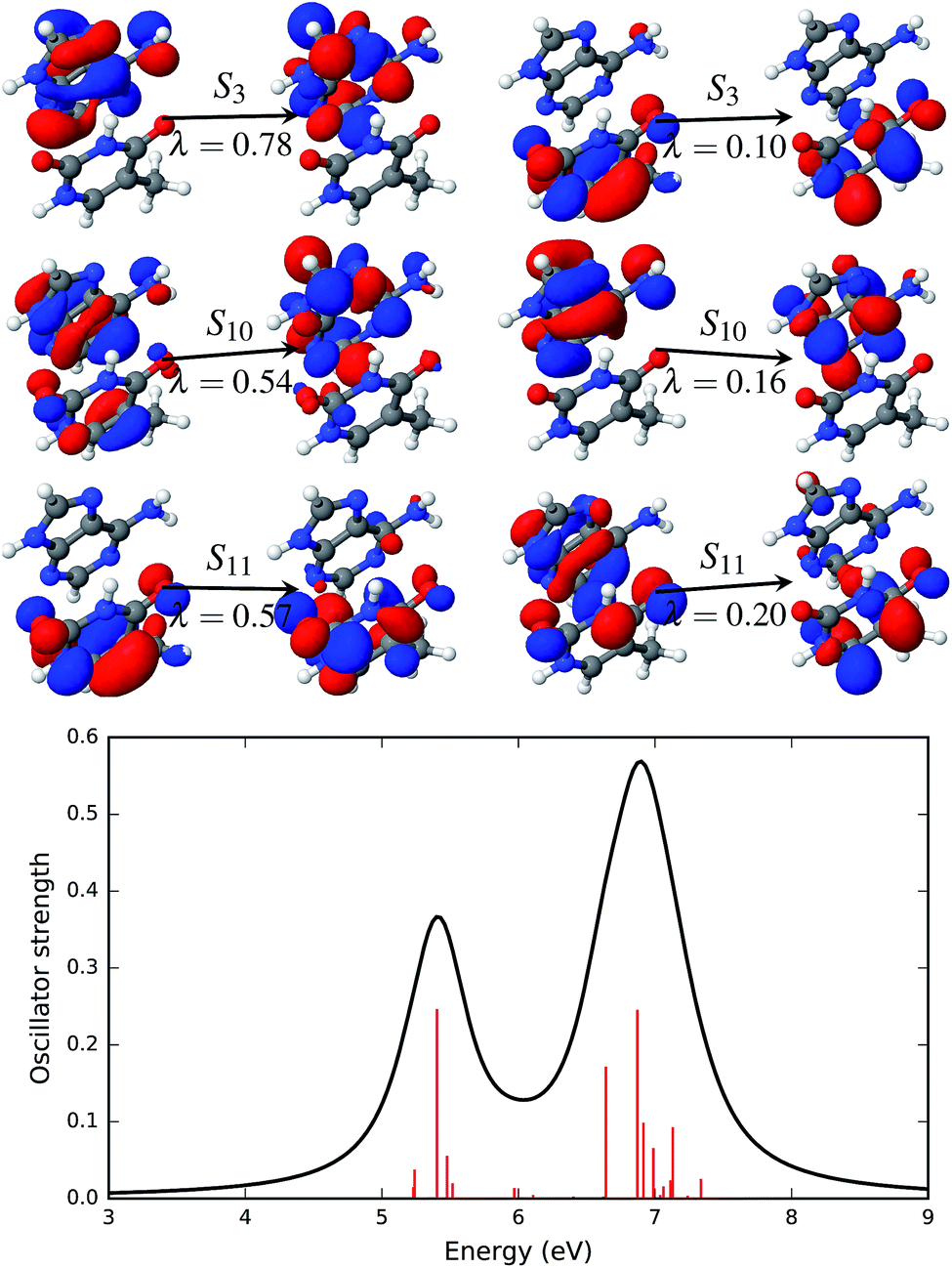
Generally, the charge transfer state appears higher in energy in comparison with that of the first bright state. This trend is also observed in AT-S. In the gas phase the first bright state is S₃ at a vertical excitation energy (VEE) of 5.4 eV. The charge transfer state, S₆, is 0.57 eV above the bright state, S₃. This agrees well with earlier calculations that used various theoretical models. For example, when using the CC2 method the state of A → T charge transfer was found to be above the bright state by values of 0.6 to 0.8 eV.^3,40,75 Other DFT functionals with long range corrections, such as M05-2X and LRC-PBE0, also correctly predicted the CT state to be above the bright state by 0.5 eV ³⁹ and 0.7 eV,⁴⁰ respectively.

The effects of hydration on the excited state characterization were also analysed using the data presented in Table 2. As mentioned earlier, the overall electronic spectrum of AT-S is red shifted in an aqueous environment. The first bright state in an aqueous environment is S₄, and is found to be 0.28 eV below the first bright state of the gas phase AT.

The effect of hydration on de-localization is significant. Five states, S₂, S₃, S₄, S₉ and S₁₀, are de-localized and their PR values range from 1.34 to 1.79 (see Table 2). In comparison, there are only three states de-localized in the gas phase. All four localized states are localized on adenine.

As in the gas phase, there is only one CT state in aqueous AT-S. The CT state, S₇, is 0.57 eV above the bright state in an aqueous environment and 0.28 eV below the bright state in the gas phase. The NTO pair and the electron–hole correlation matrices (Ω matrices) are shown in Fig. 4b. Unlike in the gas phase, charge transfer in the aqueous phase is from the ground state of thymine to the excited state of adenine. This result is in stark contrast with the results presented in ref. 35 and 37. Their calculations, using a PCM model that did not consider any geometry relaxation, did not show any change of direction in charge transfer. Our calculations show that this is an effect of the geometry relaxation of stacked base pairs in solution and consequential dipole interactions with the solvent molecules. Furthermore, in order to clarify the role of geometry relaxation in solution, we calculated the constrained gas phase base pair structure in solution, using the same ωB97X/cc-pVTZ model. In this case, the charge transfer direction is from the ground state of adenine to the excited state of thymine, as in the gas phase. An electron density plot of the charge transfer state of this configuration along with the electron–hole correlation plot analogous to the plot in Fig. 4b is provided in the ESI.† However in both cases the states are highly localized in one fragment. Our results once again show that structural relaxation influences the excited state characteristics of the base pair significantly, and that a bulk solvent model such as PCM is incapable of capturing this effect.

Ab initio calculations and systematic analysis in ref. 76 showed that non-radiative decay, via conical intersections with the ground state potential energy surface, is the low energy pathway of photo-deactivation of the individual DNA bases thymine, cytosine, adenine and guanine following UV excitation. In base-pairs in both the WC and stacked configurations, electron driven proton transfer (EDPT) has been identified as an efficient deactivation pathway following photoexcitation.⁷⁶ The driving force of EDPT is the CT state, where charge separation between the fragments leads to exited state proton transfer. A series of ab initio studies have identified CT states in AT-WC,^3,37,77 guanine–cytosine WC¹⁹ as well as in AT-S³⁵ base pairs. Here we identify the CT states of the AT-S base pair both in the gas phase and in solution. EDPT via a CT state can provide an efficient non-radiative path to the ground state after UV excitation.⁷⁶

There are significant excitonic coupling states of AT-S in the gas phase. Excitonic couplings are essential to the understanding of the photophysics of multichromophoric systems such as DNA bases, because the magnitude of the coupling determines the rate of excitation energy transfer between the donor and acceptor. The upper limit for coupling can simply be estimated⁷⁸ as 0.005 eV. Our results overestimate the magnitude of excitonic coupling compared to the data obtained by more sophisticated MS-CASPT2 calculations.⁷⁸ Such a trend for TD-DFT calculations, which overestimate the magnitude of excitonic coupling, has also been found for stacked DNA base homodimers.^78,79 Interestingly, the solvation effect significantly lowers the magnitude of excitonic coupling between the S₁ and S₂ states in AT-S, but shows significant coupling between the S₃ and S₄ states. The excitonic coupling between S₉ and S₁₀ is significant in both the gas phase and in solution.

AT-WC. The excited states of the AT-WC configuration in both the gas phase and in an aqueous environment were characterized by the quantitative descriptors presented in Table 3. The first eight excited states of the gas phase AT-WC base pairs are highly localized and their PR values do not exceed 1.13. In contrast, the S₉ and S₁₀ states are highly de-localized, with the transition involving both fragments. In particular, S₁₀ is a state that involves around four pairs of NTOs (PR_NTO ≈ 3.52). However, all of these transitions are local Frenkel-type transitions and there is no mixing with the CT type transition, as reflected by the low COH values (≈1). In contrast, S₉ is a mixture of Frenkel-type and CT-type transitions (COH ≈ 1.3).

Table 3 Excitation energies (ΔE, eV), oscillator strengths (f) and statistical descriptors (e.g. Ω, POS, PR, CT and COH, see the text for details) for the first 10 excited states of AT-WC in the gas phase (AT) and in solution (AT_SOL)

State	ΔE (eV) (transition type)		f		Ω		POS		PR		CT		COH
	AT	ATSOL	AT	ATSOL	AT	ATSOL	AT	ATSOL	AT	ATSOL	AT	ATSOL	AT	ATSOL
S1	5.34 (ππ*)	4.83 (ππ*)	0.19	0.00	0.94	0.92	1.95	1.01	1.12	1.02	0.01	0.02	1.01	1.02
S2	5.43 (nπ*)	4.98 (nπ*)	0.00	0.00	0.91	0.92	1.98	1.99	1.05	1.02	0.05	0.02	1.05	1.02
S3	5.50 (ππ*)	4.99 (ππ*)	0.31	0.17	0.91	0.92	1.06	2.00	1.13	1.00	0.00	0.00	1.00	1.00
S4	5.52 (ππ*)	5.13 (ππ*)	0.04	0.29	0.92	0.88	1.00	1.00	1.01	1.00	0.01	0.00	1.01	1.00
S5	5.72 (nπ*)	5.49 (nπ*)	0.00	0.02	0.92	0.87	1.04	1.02	1.08	1.04	0.08	0.04	1.08	1.04
S6	6.27 (nπ*)	5.53 (nπ*)	0.00	0.00	0.91	0.89	1.04	1.02	1.09	1.05	0.08	0.05	1.08	1.05
S7	6.57 (nπ*)	6.24 (nπ*)	0.00	0.00	0.81	0.92	2.00	1.03	1.01	1.06	0.01	0.06	1.01	1.06
S8	6.62 (nπ*)	6.32 (nπ*)	0.00	0.00	0.89	0.86	1.04	1.99	1.09	1.03	0.08	0.03	1.08	1.03
S9	6.72 (ππ*)	6.48 (ππ*)	0.05	0.41	0.85	0.86	1.58	1.01	1.92	1.03	0.14	0.03	1.31	1.03
S10	6.91 (ππ*)	6.54 (ππ*)	0.29	0.01	0.94	0.96	1.54	1.50	1.99	1.00	0.01	1.00	1.01	1.00
S11	6.97 (ππ*)	6.65 (ππ*)	0.01	0.06	0.80	0.92	1.50	2.00	1.01	1.01	0.99	0.01	1.01	1.01

---

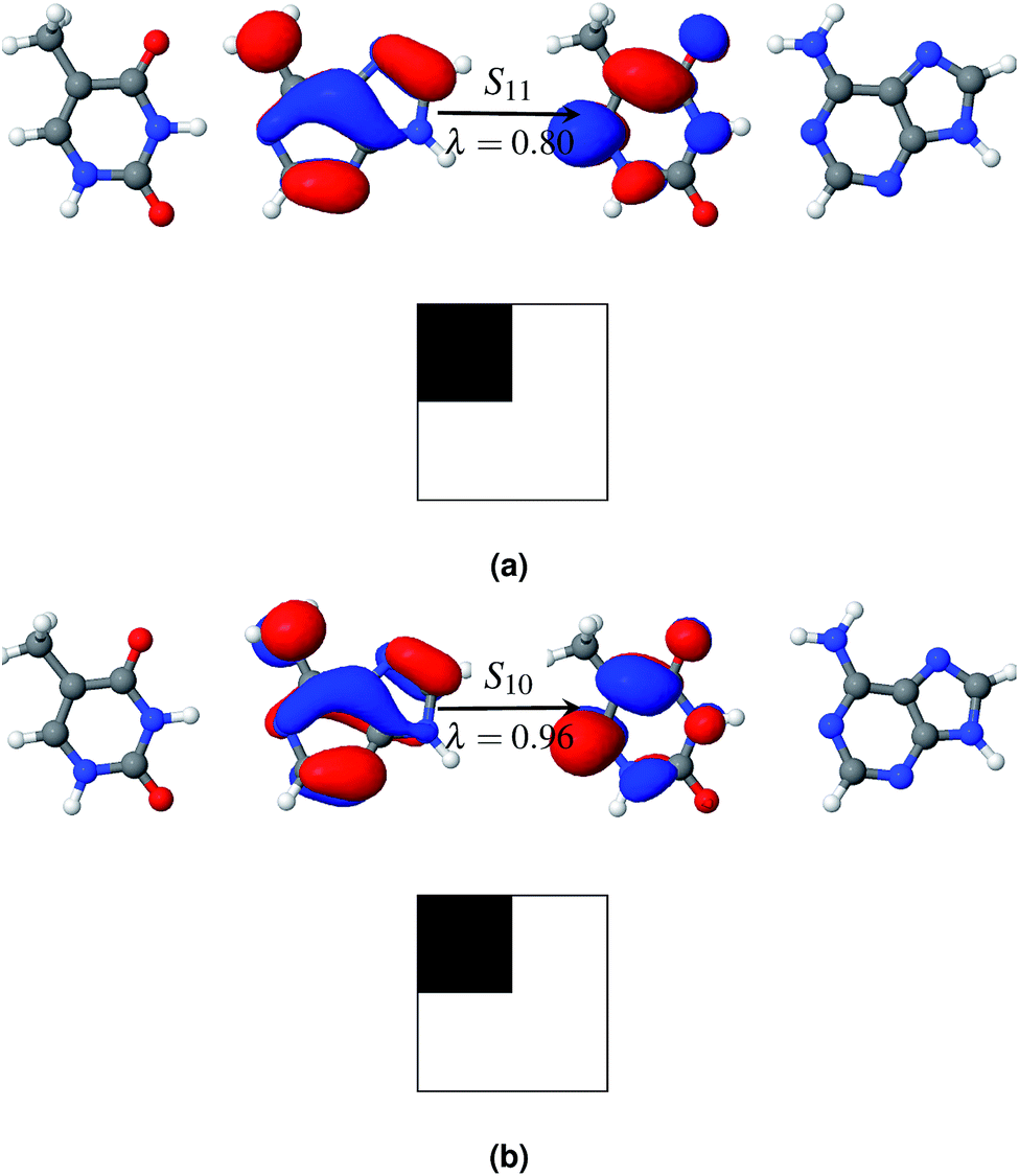
Fig. 5a shows that the S₁₁ state is a CT-type state (CT = 0.99) where charge is transferred from the ground state of adenine to the excited state of thymine. Both of the ground and excited state orbitals are π orbitals. Hence this is an Aπ → Tπ* transition. This CT state is described by one pair of NTOs, as shown in Fig. 5a. This CT state is immediately (0.06 eV) above the bright state. However among the 1st eleven states there are two more (S₁ and S₃) bright states.

Fig. 5 Charge transfer states of AT-WC in the gas phase (a) and in solution (b). The symbol above the arrow indicates the singlet excited state that is described by the NTO pairs presented in the figure. The panel to the left of the arrow shows the hole density and the panel to the right of the arrow shows the particle density. The symbol, λ, below the arrow gives the weight of the respective configuration. Electron–hole correlation plots (Ω matrix) of the charge transfer excitation states are presented at the bottom of each figure. The Ω matrix is a 2 × 2 matrix here as the AT dimer is divided into two fragments. Adenine and thymine are defined as fragments 1 and 2, respectively.

Hydration affects the excited states of the WC configuration of the AT base pair somewhat differently than the stacked configuration. All of the first eleven excited states of AT-WC in an aqueous environment are localized and their PR values do not exceed 1.06 (see Table 3). In comparison, two excited states in the gas phase are highly de-localized, as discussed above. S₁₀ is the CT state in the aqueous environment. Like the CT state in the gas phase, this is an Aπ → Tπ* transition state (see Fig. 5b), with the hole and particle densities localized on the ground state of adenine and excited state of thymine, respectively. As in the gas phase, the CT state in the aqueous environment is 0.06 eV higher than the bright state. However, the CT state in the aqueous environment is 0.37 eV lower than the bright state in the gas phase, as hydration forces a red shift on the overall electronic spectrum. The identified CT state could lead to viable non-radiative deactivation pathways via EDPT.^37,76,77

Overall, hydration affects the charge de-localization in the excited states of the AT-S and AT-WC configurations in different ways. The number of inter-fragment de-localized states (i.e. states in which the charge is de-localized over both molecular fragments) increases significantly in the aqueous phase in comparison with the gas phase AT-S. However, in AT-WC most of the states remain localized in one molecular fragment. A close visual inspection of the hole and particle density distribution in terms of the NTOs suggests some intra-molecular de-localizations as a result of the hydration effects. The discrepancies in the number of de-localized states of AT-S and AT-WC in an aqueous environment can be explained by considering the number of potential hydrogen bonding interactions that is plausible for each configuration. In AT-S both the purine in adenine and the pyrimidine ring in thymine are available for potential hydrogen bonding interactions in an aqueous environment. On the other hand, adenine and thymine in the AT-WC configuration are already involved in three hydrogen bonding interactions through adenine’s five-membered ring and thymine’s pyrimidine ring and methyl group.

There is no significant excitonic coupling between the low lying excited states of AT-WC both in the gas and condensed phase. The magnitude of coupling between S₃ and S₄ in the gas phase and S₂ and S₃ in solution can be estimated as 0.01 eV and 0.005 eV, respectively.

3.5 Natural transition orbitals (NTOs)

Natural transition orbitals create a compact representation of an electronic excited state.⁴⁷ Natural transition orbitals can be obtained by carrying out a singular value decomposition of the one-particle transition density matrix (1-TDM).^48,71 The concept of natural transition orbitals helps in the understanding of the physical principles underlying the electronic transition. The number of configurations required for an adequate description of the features of a transition can be significantly reduced with NTOs. The response vectors of the excited state configurations of the first twenty singlet states were calculated using time dependent density functional theory.

Fig. 6–9 show the electronic spectra and NTOs with significant transition strengths. The symbols and numbers above and below the arrows in the NTOs in Fig. 6–9 represent the corresponding excited states and the weights (λ_i) of the transitions, respectively. Significant oscillator strengths of the singlet states are indicated by the red vertical lines in the electronic spectra. The electronic spectra were generated using the Gaussian convolution with 0.5 FWHM.

Fig. 6 Natural transition orbitals (NTOs, upper panel) that describe the brightest excited states of the AT-S absorption spectrum in the gas phase along with the simulated absorption spectrum (lower panel). The symbol above the arrow indicates the singlet excited state that is described by the NTO pairs presented in the figure. The panel to the left of the arrow shows the hole density and the panel to the right of the arrow shows the particle density. The symbol, λ, below the arrow gives the weight of the respective configuration. The electronic transitions, quantified by the oscillator strengths, are shown as vertical red bars in the lower panel.

Fig. 7 Natural transition orbitals (NTOs, upper panel) that describe the brightest excited states of the AT-S absorption spectrum in solution along with the simulated absorption spectrum (lower panel). The symbol above the arrow indicates the singlet excited state that is described by the NTO pairs presented in the figure. The panel to the left of the arrow shows the hole density and the panel to the right of the arrow shows the particle density. The symbol, λ, below the arrow gives the weight of the respective configuration. The electronic transitions, quantified by the oscillator strengths, are shown as vertical red bars in the lower panel.

Fig. 8 Natural transition orbitals (NTOs, upper panel) that describe the brightest excited states of the AT-WC absorption spectrum in the gas phase along with the simulated absorption spectrum (lower panel). The symbol above the arrow indicates the singlet excited state that is described by the NTO pairs presented in the figure. The panel to the left of the arrow shows the hole density and the panel to the right of the arrow shows the particle density. The symbol, λ, below the arrow gives the weight of the respective configuration. The electronic transitions, quantified by the oscillator strengths, are shown as vertical red bars in the lower panel.

Fig. 9 Natural transition orbitals (NTOs, upper panel) that describe the brightest excited states of the AT-WC absorption spectrum in solution along with the simulated absorption spectrum (lower panel). The symbol above the arrow indicates the singlet excited state that is described by the NTO pairs presented in the figure. The panel to the left of the arrow shows the hole density and the panel to the right of the arrow shows the particle density. The symbol, λ, below the arrow gives the weight of the respective configuration. The electronic transitions, quantified by the oscillator strengths, are shown as vertical red bars in the lower panel.

The first significant transition in the AT base pair with a stacked configuration is the transition to the S₃ singlet excited state (see Fig. 6) at 5.40 eV (229.6 nm). This transition is described by two sets of NTOs with weights of 0.78 and 0.10. In both sets of NTOs the hole and particle densities are on the same fragment, i.e. on adenine for the NTO pair with λ = 0.78 and thymine for the NTO pair with λ = 0.10. This type of transition thus constitutes a Frankel type local transition. The next two significant excited states, S₁₀ at 6.64 eV (186.7 nm) and S₁₁ at 6.87 eV (180.5 nm), are also described by two pairs of NTOs. There is some de-localization of the hole densities spread on both the adenine and thymine fragments in both of these excited states. All three of these bright transitions are of a ππ* type. There are two more, S₅ and S₆, ππ* states with low oscillator strengths that are below the energy range of 6.64 eV. All other states, except for S₁, are localized nπ* states.

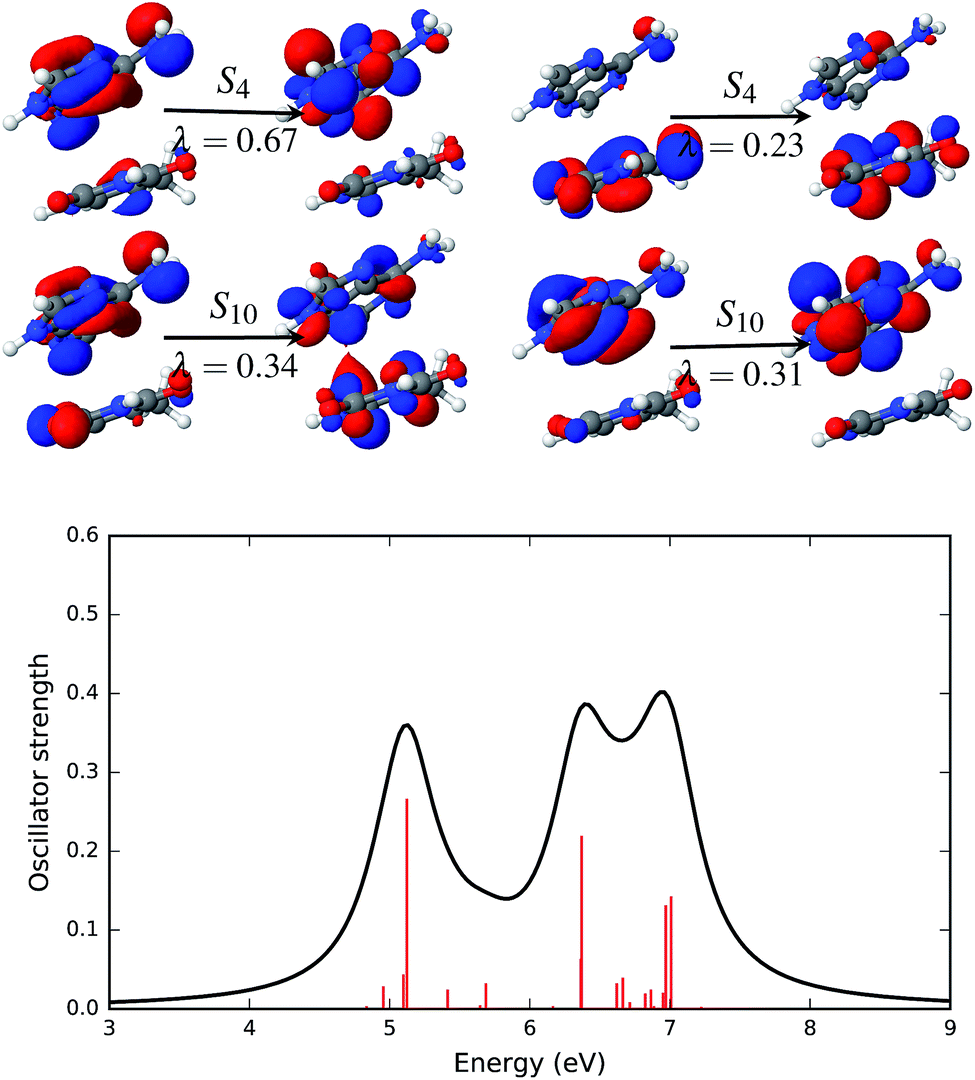
The effect of the solvent environment on the excited state of the AT base pair is presented in Fig. 7. As mentioned above, solvation effects broaden the electronic spectra in the UV range. Significant excited states with high oscillator strengths are the singlet states S₄, S₁₀, S₁₈ and S₁₉. The dominant NTO pairs of the S₄ and S₁₀ states are shown in Fig. 7. The S₄ state is represented by two transitions. These transitions involve orbitals that are localized on either adenine (NTOs with λ = 0.67) or thymine (λ = 0.23). The S₁₀ state is represented by two NTO pairs with almost equal weight, λ = 0.34 and λ = 0.31. The transition with λ = 0.31 involves orbitals that are localized on adenine. However, the other dominant transition in the S₁₀ state involves particle orbitals that are de-localized over both the adenine and thymine fragments. This sort of partial charge transfer is facilitated by the presence of solvent water molecules.

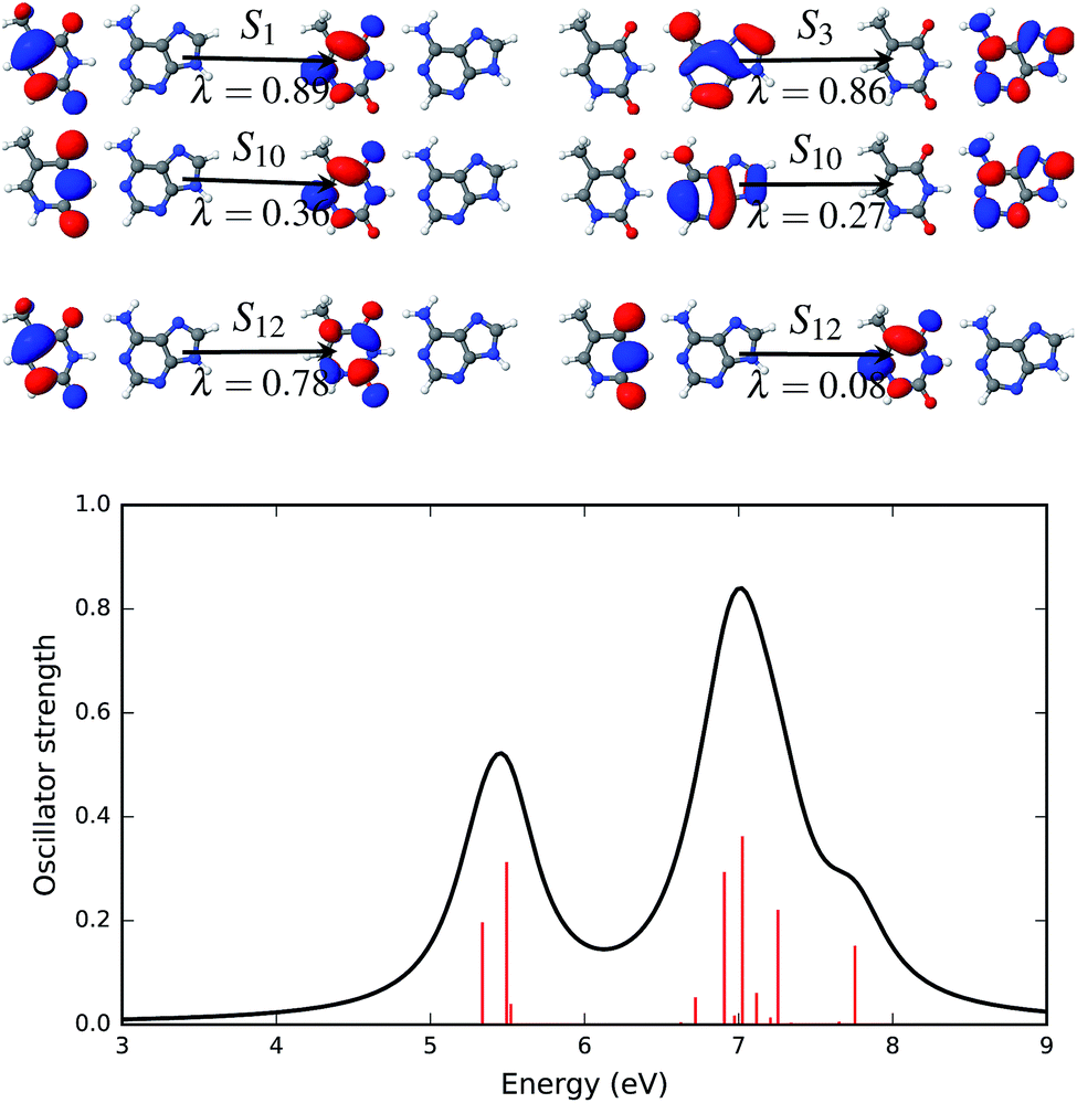
NTOs that describe the excited states of the AT base pair in the canonical Watson–Crick configuration are presented in Fig. 8. The electronic spectrum of this configuration has at least four significant excited states with high oscillator strengths. The first (S₁) and third (S₃) excited states are completely described by a single set of NTOs. Both of these states are described by a transition that involves an orbital localized on a single fragment of the base pair. The NTO pair representing the first (S₁) and third (S₃) states is localized on thymine and adenine, respectively. The excited states S₁₀ and S₁₂ involve two pairs of dominant NTOs. In both states and both NTOs, hole and particle orbitals are localized on the same fragment, i.e. either on thymine (S₁₀, λ = 0.36 and S₁₂, λ = 0.78, 0.08) or on adenine (S₁₀, λ = 0.27).

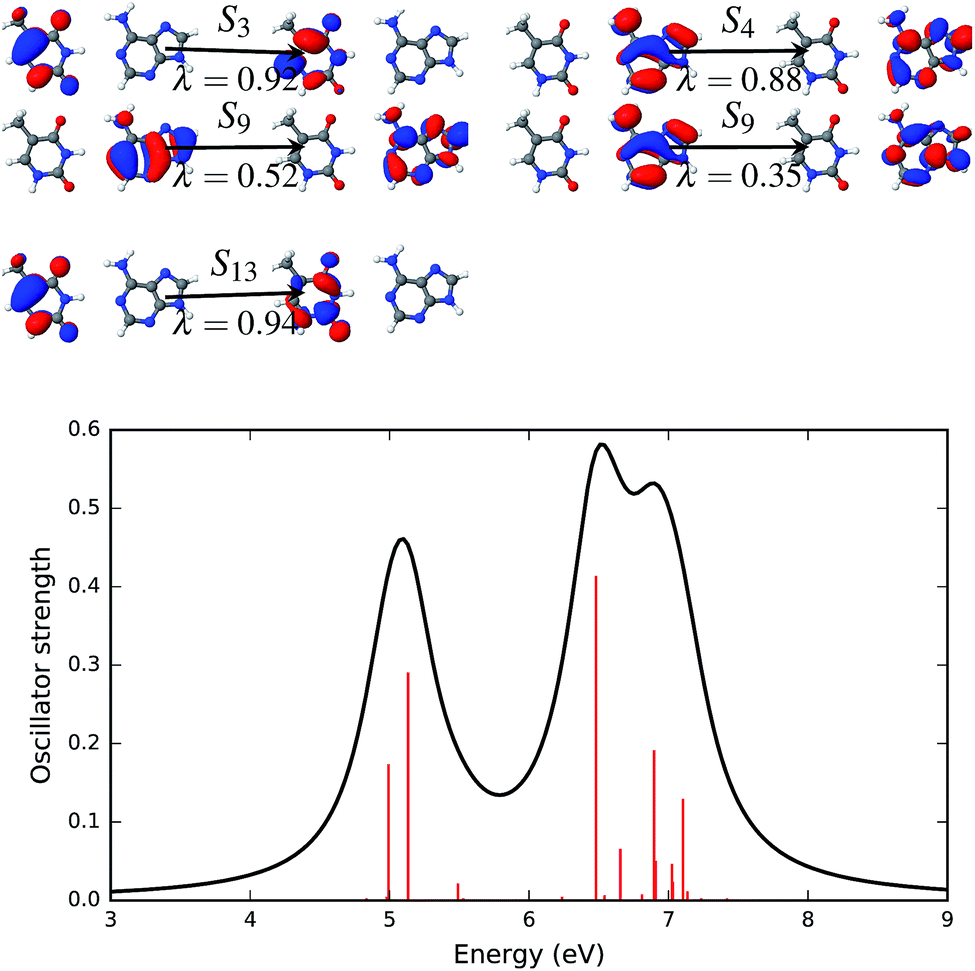
The four most significant excited states with high oscillator strengths that dominate the electronic spectrum of the AT base pair in the Watson–Crick configuration and surrounded by water molecules are S₃, S₄, S₉ and S₁₃. NTOs representing these states and the electronic spectrum are shown in Fig. 9. Like the solvent effects in the stacked configuration, the electronic spectrum of the canonical base pair configuration is also broadened near the 7 eV energy band. The S₃, S₄ and S₁₃ states are described by a single pair of NTOs. However, two NTO pairs are needed to describe the S₉ state.

The inclusion of solvent effects by an effective fragment potential significantly stabilizes both the nπ* and ππ* states of AT dimers in both of the configurations considered here. Our results agree with the data presented in ref. 37, where the bulk solvent effects were modelled using PCM and it was found that the bright ππ* states of the AT-WC configuration were stabilized by a polar solvent. However our results disagree with the data presented in ref. 35 and 80. The discrepancies with the results in ref. 35 were already discussed above. In ref. 80, vertical excitations of 4-aminopyrimidine were investigated by means of microsolvation using two- and four-water models and continuum solvation models. Therefore, the effects of stacking and WC hydrogen bonding, as well as the effect of the geometry relaxation of base pairs in solution, are absent in this model. We assume that the strong stabilization effect of excited states in solution in our study is due to dimer relaxation and hydrogen bonding interactions in solution. Such interactions affect the energies of both nπ* and ππ* type excitations.

4 Conclusion

A systematic analysis of the excited state characteristics of the DNA base pair adenine–thymine in stacked and Watson–Crick hydrogen bonded configurations has been carried out in this study. The analysis based on the one-electron transition density matrix (1TDM) demonstrates its advantages for quantitative characterization of the excited state. A compact representation of the characteristics of the excited states was provided by a number of descriptors. Analysis of the bright states in terms of natural transition orbitals showed that each state can be described by at most two sets of NTOs.

We have thoroughly analysed the extent of de-localization and the charge transfer character of excited states in the near- and far-ultraviolet region of the electromagnetic spectrum. Such an analysis and accurate identification of the charge transfer states are essential for understanding the photo-stability of DNA, as these properties influence the interactions of DNA bases in the aftermath of ultraviolet photo-excitation. Analogous studies on core-excitation will shed light on the interactions in high energy X-ray excitation. Additionally, localized Frenkel type as well as de-localized states involving multiple molecular fragments were also identified.

The effect of hydration on the excited state characteristics of DNA bases was also analysed. It was found that hydration influences de-localization in different ways for the AT-S and AT-WC configurations. In AT-S, the hydration effect results in significant inter-fragment de-localization, whereas in AT-WC de-localization is intra-fragment. A thorough understanding of the defect dynamics in DNA is highly dependant upon such assignments of electronically excited states in terms of their localized or de-localized characteristics. Our results further support the experimental and theoretical findings that the effect of solvent on excitation in the mid and far ultraviolet energy ranges results in a red shift as well as a lower absorbance in the electronic spectra.

Significantly, we identified that geometry relaxation in solution plays a very important role in defining the excited state characteristics of base pairs in both the stacked and WC configurations. In contrast to the results obtained using a bulk solvent model such as PCM, our results show that in the solution phase the charge transfer direction can be changed compared to that of the gas phase. This effect is a result of the changing dipole in the relaxed structure in solution and explicit solute–solvent interactions that we considered through the use of effective field potentials. We conclude that implicit solvent models that exclude non-electrostatic solute–solvent interactions are not adequate for excited state characterization of DNA base pairs.

Additionally, the long-range corrected hybrid density functional ωB97X was tested for simulation of the excited states of DNA bases and was found to be a reasonable option for large scale TDDFT calculations, since it predicts charge transfer states rather accurately.

Acknowledgements

The authors acknowledge the support of the Australian Research Council Centre of Excellence in Advanced Molecular Imaging. This research was supported by the Victorian Life Sciences Computation Initiative (VLSCI) grant number UOM0006 on its Snowy Computing Facility at the University of Melbourne, an initiative of the Victorian Government, Australia.

References

1. M. Barbatti, A. C. Borin and S. Ullrich, Photoinduced Phenomena in Nucleic Acids II, Springer, 2015, vol. 355, pp. 39–87.
2. J. Cadet and R. J. Wagner, Cold Spring Harbor Perspect. Biol., 2013, 5, 1–18.
3. S. Perun, A. L. Sobolewski and W. Domcke, J. Phys. Chem. A, 2006, 110, 13238–13244.
4. L. Martinez-Fernandez, Y. Zhang, K. de La Harpe, A. A. Beckstead, B. Kohler and R. Improta, Phys. Chem. Chem. Phys., 2016, 18, 21241–21245.
5. D. B. Bucher, B. M. Pilles, T. Carell and W. Zinth, Proc. Natl. Acad. Sci. U. S. A., 2014, 111, 4369–4374.
6. P. M. Keane, M. Wojdyla, G. W. Doorley, J. M. Kelly, I. P. Clark, A. W. Parker, G. M. Greetham, M. Towrie, L. M. Magno and S. J. Quinn, Phys. Chem. Chem. Phys., 2012, 14, 6307.
7. Z. Benda and P. G. Szalay, Phys. Chem. Chem. Phys., 2016, 18, 23596–23606.
8. C. E. Crespo-Hernandez, B. Cohen, P. M. Hare and B. Kohler, Chem. Rev., 2004, 104, 1977–2019.
9. J. M. L. Pecourt, J. Peon and B. Kohler, J. Am. Chem. Soc., 2001, 123, 5166.
10. D. Markovitsi, F. Talbot, T. Gustavsson, D. Onidas, E. Lazzarotto and S. Marguet, Nature, 2006, 441, E7.
11. G. W. Doorley, M. Wojdyla, G. W. Watson, M. Towrie, A. W. Parker, J. M. Kelly and S. J. Quinn, J. Phys. Chem. Lett., 2013, 4, 2739–2744.
12. T. Takaya, C. Su, K. de La Harpe, C. E. Crespo-Hernandez and B. Kohler, Proc. Natl. Acad. Sci. U. S. A., 2008, 105, 10285–10290.
13. D. Markovitsi, D. Onidas, T. Gustavsson, F. Talbot and E. Lazzarotto, J. Am. Chem. Soc., 2005, 127, 17130–17131.
14. A. Rich and I. Tinoco, J. Am. Chem. Soc., 1960, 82, 6409–6411.
15. J. Eisinger and R. G. Shulman, Science, 1968, 161, 1311–1319.
16. A. A. Beckstead, Y. Zhang, M. S. de Vries and B. Kohler, Phys. Chem. Chem. Phys., 2016, 18, 24228–24238.
17. W. J. Schreier, P. Gilch and W. Zinth, Annu. Rev. Phys. Chem., 2015, 66, 497–519.
18. M. Towrie, G. W. Doorley, M. W. George, A. W. Parker, J. Quinn and J. M. Kelly, Analyst, 2009, 1265–1273.
19. K. Röttger, H. J. B. Marroux, M. P. Grubb, P. M. Coulter, H. Böhnke, A. S. Henderson, M. C. Galan, F. Temps, A. J. Orr-Ewing and G. M. Roberts, Angew. Chem., Int. Ed., 2015, 54, 14719–14722.
20. K. Röttger, H. J. Marroux, A. F. M. Chemin, E. Elsdon, T. A. A. Oliver, S. T. G. Street, A. S. Henderson, M. C. Galan, A. J. Orr-Ewing and G. M. Roberts, J. Phys. Chem. B, 2017, 121(17), 4448–4455.
21. C. Su, C. T. Middleton and B. Kohler, J. Phys. Chem. B, 2012, 116, 10266–10274.
22. A. W. Parker, C. Y. Lin, M. W. George, M. Towrie and M. K. Kuimova, J. Phys. Chem. B, 2010, 114, 3660–3667.
23. M. K. Shukla and J. Leszczynski, J. Biomol. Struct. Dyn., 2007, 25, 37–41.
24. R. Improta, F. Santoro and L. Blancafort, Chem. Rev., 2016, 116, 3540–3593.
25. M. Barbatti, A. C. Borin and S. Ullrich, Top. Curr. Chem., 2015, 355, 1–32.
26. M. Barbatti and H. Lischka, J. Am. Chem. Soc., 2008, 130, 6831–6839.
27. S. Perun, a. L. Sobolewski and W. Domcke, Mol. Phys., 2006, 104, 1113–1121.
28. H. R. Hudock, B. G. Levine, A. L. Thompson, H. Satzger, D. Townsend, N. Gador, S. Ullrich, A. Stolow and T. J. Martinez, J. Phys. Chem. A, 2007, 111, 8500–8508.
29. C. M. Marian, J. Chem. Phys., 2005, 122, 104314.
30. J. J. Szymczak, M. Barbatti, J. T. S. Hoo, J. A. Adkins, T. L. Windus, D. Nachtigallova and H. Lischka, J. Phys. Chem. A, 2009, 113, 12686–12693.
31. O. Christiansen, H. Koch and P. Jorgensen, Chem. Phys. Lett., 1995, 243, 409–418.
32. G. Groenhof, L. V. Schäfer, M. Boggio-Pasqua, M. Goette, H. Grubmüller and M. A. Robb, J. Am. Chem. Soc., 2007, 129, 6812–6819.
33. P. G. Szalay, T. Watson, A. Perera, V. Lotrich and R. J. Bartlett, J. Phys. Chem. A, 2013, 117, 3149–3157.
34. C. R. Kozak, K. A. Kistler, Z. Lu and S. Matsika, J. Phys. Chem. B, 2010, 114, 1674–1683.
35. A. J. A. Aquino, D. Nachtigallova, P. Hobza, D. G. Truhlar, C. Hättig and H. Lischka, J. Comput. Chem., 2010, 31, 2967–2970.
36. T. Kubar and M. Elstner, J. Phys. Chem. B, 2008, 112, 8788–8798.
37. M. Dargiewicz, M. Biczysko, R. Improta and V. Barone, Phys. Chem. Chem. Phys., 2012, 14, 8981.
38. F. Plasser, M. Barbatti, A. J. A. Aquino and H. Lischka, Theor. Chem. Acc., 2012, 131, 1–14.
39. F. Santoro, V. Barone and R. Improta, ChemPhysChem, 2008, 9, 2531–2537.
40. A. W. Lange and J. M. Herbert, J. Am. Chem. Soc., 2009, 131, 3913–3922.
41. A. Czader and E. R. Bittner, J. Chem. Phys., 2008, 128, 035101.
42. S. Tonzani and G. C. Schatz, J. Am. Chem. Soc., 2008, 130, 7607–7612.
43. E. Emanuele, D. Markovitsi, P. Millie and K. Zakrzewska, ChemPhysChem, 2005, 6, 1387–1392.
44. E. Emanuele, K. Zakrzewska, D. Markovitsi, R. Lavery and P. Millie, J. Phys. Chem. B, 2005, 109, 16109–16118.
45. D. Ghosh, D. Kosenkov, V. Vanovschi, J. Flick, I. Kaliman, Y. Shao, A. T. B. Gilbert, A. I. Krylov and L. V. Slipchenko, J. Comput. Chem., 2013, 34, 1060–1070.
46. S. A. Bappler, F. Plasser, M. Wormit and A. Dreuw, Phys. Rev. A, 2014, 90, 052521.
47. F. Plasser, M. Wormit and A. Dreuw, J. Chem. Phys., 2014, 141, 0–13.
48. T. Etienne, J. Chem. Phys., 2015, 142, 244103.
49. F. Plasser, S. A. Bäppler, M. Wormit and A. Dreuw, J. Chem. Phys., 2014, 141, 024107.
50. S. Chopra, RSC Adv., 2016, 6, 20565–20570.
51. C. Jamorski, M. E. Casida and D. R. Salahub, J. Chem. Phys., 1996, 104, 5134–5147.
52. M. Petersilka, U. J. Gossmann and E. K. U. Gross, Phys. Rev. Lett., 1996, 76, 1212–1215.
53. R. Bauernschmitt and R. Ahlrichs, Chem. Phys. Lett., 1996, 256, 454–464.
54. D. J. Tozer and N. C. Handy, J. Chem. Phys., 1998, 109, 10180–10189.
55. A. Dreuw, J. L. Weisman and M. Head-Gordon, J. Chem. Phys., 2003, 119, 2943.
56. B. Champagne, E. A. Perpete, S. J. A. van Gisbergen, E.-J. Baerends, J. G. Snijders, C. Soubra-Ghaoui, K. A. Robins and B. Kirtman, J. Chem. Phys., 1998, 109, 10489–10498.
57. T. Leininger, H. Stoll, H. J. Werner and A. Savin, Chem. Phys. Lett., 1997, 275, 151–160.
58. H. Iikura, T. Tsuneda, T. Yanai and K. Hirao, J. Chem. Phys., 2001, 115, 3540–3544.
59. J.-D. Chai and M. Head-Gordon, J. Chem. Phys., 2008, 128, 084106.
60. A. Y. Sokolov and H. F. Schaefer, Dalton Trans., 2011, 40, 7571–7582.
61. T. H. Dunning, J. Chem. Phys., 1989, 90, 1007–1023.
62. J. Bloino, A. Baiardi and M. Biczysko, Int. J. Quantum Chem., 2016, 116, 1543–1574.
63. J. Bloino, M. Biczysko, F. Santoro and V. Barone, J. Chem. Theory Comput., 2010, 6, 1256–1274.
64. P. Jurecka, J. Sponer, J. Cerny and P. Hobza, Phys. Chem. Chem. Phys., 2006, 8, 1985–1993.
65. P. Jurecka and P. Hobza, J. Am. Chem. Soc., 2003, 125, 15608–15613.
66. A. DeFusco, N. Minezawa, L. V. Slipchenko, F. Zahariev and M. S. Gordon, J. Phys. Chem. Lett., 2011, 2, 2184–2192.
67. IQmol: The smart choice in molecular visualization software, http://www.iqmol.com.
68. A. V. Luzanov, J. Struct. Chem., 2002, 43, 711–720.
69. R. L. Martin, J. Chem. Phys., 2003, 118, 4775–4777.
70. A. T. Amos and G. G. Hall, Proc. Roy. Soc. Lond. Math. Phys. Sci., 1961, 263, 483–493.
71. F. Plasser, R. Crespo-Otero, M. Pederzoli, J. Pittner, H. Lischka and M. Barbatti, J. Chem. Theory Comput., 2014, 10, 1395–1405.
72. Y. Shao, Z. Gan, E. Epifanovsky, A. T. B. Gilbert, M. Wormit, J. Kussmann, A. W. Lange, A. Behn, J. Deng, X. Feng, D. Ghosh, M. Goldey, P. R. Horn, L. D. Jacobson, I. Kaliman, R. Z. Khaliullin, T. Kus, A. Landau, J. Liu, E. I. Proynov, Y. M. Rhee, R. M. Richard, M. A. Rohrdanz, R. P. Steele, E. J. Sundstrom, I. I. I. Woodcock, H. Lee, P. M. Zimmerman, D. Zuev, B. Albrecht, E. Alguire, B. Austin, G. J. O. Beran, Y. A. Bernard, E. Berquist, K. Brandhorst, K. B. Bravaya, S. T. Brown, D. Casanova, C.-M. Chang, Y. Chen, S. H. Chien, K. D. Closser, D. L. Crittenden, M. Diedenhofen, A. DiStasio Robert, H. Do, A. D. Dutoi, R. G. Edgar, S. Fatehi, L. Fusti-Molnar, A. Ghysels, A. Golubeva-Zadorozhnaya, J. Gomes, M. W. D. Hanson-Heine, P. H. P. Harbach, A. W. Hauser, E. G. Hohenstein, Z. C. Holden, T.-C. C. Jagau, H. Ji, B. Kaduk, K. Khistyaev, J. J. J. J. Kim, J. J. J. J. Kim, R. A. King, P. Klunzinger, D. Kosenkov, T. Kowalczyk, C. M. Krauter, K. U. Lao, A. D. A. D. A. D. Laurent, K. V. Lawler, S. V. Levchenko, C. Y. Lin, F. Liu, E. Livshits, R. C. Lochan, A. Luenser, P. Manohar, S. F. Manzer, S.-P. Mao, N. Mardirossian, A. V. Marenich, S. A. Maurer, N. J. Mayhall, E. Neuscamman, C. M. Oana, R. Olivares-Amaya, D. P. O’Neill, J. A. Parkhill, T. M. Perrine, R. Peverati, A. Prociuk, D. R. Rehn, E. Rosta, N. J. Russ, S. M. Sharada, S. Sharma, D. W. Small, A. Sodt, T. Kuś, A. Landau, J. Liu, E. I. Proynov, Y. M. Rhee, R. M. Richard, M. A. Rohrdanz, R. P. Steele, E. J. Sundstrom, H. L. Woodcock, P. M. Zimmerman, D. Zuev, B. Albrecht, E. Alguire, B. Austin, G. J. O. Beran, Y. A. Bernard, E. Berquist, K. Brandhorst, K. B. Bravaya, S. T. Brown, D. Casanova, C.-M. Chang, Y. Chen, S. H. Chien, K. D. Closser, D. L. Crittenden, M. Diedenhofen, R. A. DiStasio, H. Do, A. D. Dutoi, R. G. Edgar, S. Fatehi, L. Fusti-Molnar, A. Ghysels, A. Golubeva-Zadorozhnaya, J. Gomes, M. W. D. Hanson-Heine, P. H. P. Harbach, A. W. Hauser, E. G. Hohenstein, Z. C. Holden, T.-C. C. Jagau, H. Ji, B. Kaduk, K. Khistyaev, J. J. J. J. Kim, J. J. J. J. Kim, R. A. King, P. Klunzinger, D. Kosenkov, T. Kowalczyk, C. M. Krauter, K. U. Lao, A. D. A. D. A. D. Laurent, K. V. Lawler, S. V. Levchenko, C. Y. Lin, F. Liu, E. Livshits, R. C. Lochan, A. Luenser, P. Manohar, S. F. Manzer, S.-P. Mao, N. Mardirossian, A. V. Marenich, S. A. Maurer, N. J. Mayhall, E. Neuscamman, C. M. Oana, R. Olivares-Amaya, D. P. O’Neill, J. A. Parkhill, T. M. Perrine, R. Peverati, A. Prociuk, D. R. Rehn, E. Rosta, N. J. Russ, S. M. Sharada, S. Sharma, D. W. Small, A. Sodt, T. Stein, D. Stück, Y.-C. Su, A. J. Thom, T. Tsuchimochi, V. Vanovschi, L. Vogt, O. Vydrov, T. Wang, M. A. Watson, J. Wenzel, A. White, C. F. Williams, J. Yang, S. Yeganeh, S. R. Yost, Z.-Q. You, I. Y. Zhang, X. Zhang, Y. Zhao, B. R. Brooks, G. K. Chan, D. M. Chipman, C. J. Cramer, W. A. Goddard, M. S. Gordon, W. J. Hehre, A. Klamt, H. F. Schaefer, M. W. Schmidt, C. D. Sherrill, D. G. Truhlar, A. Warshel, X. Xu, A. Aspuru-Guzik, R. Baer, A. T. Bell, N. A. Besley, J.-D. Chai, A. Dreuw, B. D. Dunietz, T. R. Furlani, S. R. Gwaltney, C.-P. Hsu, Y. Jung, J. Kong, D. S. Lambrecht, W. Liang, C. Ochsenfeld, V. A. Rassolov, L. V. Slipchenko, J. E. Subotnik, T. Van Voorhis, J. M. Herbert, A. I. Krylov, P. M. Gill, M. Head-Gordon, T. Kus, A. Landau, J. Liu, E. I. Proynov, Y. M. Rhee, R. M. Richard, M. A. Rohrdanz, R. P. Steele, E. J. Sundstrom, I. I. I. Woodcock, H. Lee, P. M. Zimmerman, D. Zuev, B. Albrecht, E. Alguire, B. Austin, G. J. O. Beran, Y. A. Bernard, E. Berquist, K. Brandhorst, K. B. Bravaya, S. T. Brown, D. Casanova, C.-M. Chang, Y. Chen, S. H. Chien, K. D. Closser, D. L. Crittenden, M. Diedenhofen, A. DiStasio Robert, H. Do, A. D. Dutoi, R. G. Edgar, S. Fatehi, L. Fusti-Molnar, A. Ghysels, A. Golubeva-Zadorozhnaya, J. Gomes, M. W. D. Hanson-Heine, P. H. P. Harbach, A. W. Hauser, E. G. Hohenstein, Z. C. Holden, T.-C. C. Jagau, H. Ji, B. Kaduk, K. Khistyaev, J. J. J. J. Kim, J. J. J. J. Kim, R. A. King, P. Klunzinger, D. Kosenkov, T. Kowalczyk, C. M. Krauter, K. U. Lao, A. D. A. D. A. D. Laurent, K. V. Lawler, S. V. Levchenko, C. Y. Lin, F. Liu, E. Livshits, R. C. Lochan, A. Luenser, P. Manohar, S. F. Manzer, S.-P. Mao, N. Mardirossian, A. V. Marenich, S. A. Maurer, N. J. Mayhall, E. Neuscamman, C. M. Oana, R. Olivares-Amaya, D. P. O’Neill, J. A. Parkhill, T. M. Perrine, R. Peverati, A. Prociuk, D. R. Rehn, E. Rosta, N. J. Russ, S. M. Sharada, S. Sharma, D. W. Small and A. Sodt, et al., Mol. Phys., 2015, 113, 184–215.
73. Jmol: an open-source Java viewer for chemical structures in 3D, http://www.jmol.org/.
74. M. Hodecker, M. Biczysko, A. Dreuw and V. Barone, J. Chem. Theory Comput., 2016, 12, 2820–2833.
75. H. T. Sun, S. A. Zhang, C. Zhong and Z. R. Sun, J. Comput. Chem., 2016, 37, 684–693.
76. B. Marchetti, T. N. Karsili, M. N. Ashfold and W. Domcke, Phys. Chem. Chem. Phys., 2016, 18, 20007–20027.
77. J. P. Gobbo, V. Saurí, D. Roca-Sanjuán, L. Serrano-Andrés, M. Merchán and A. C. Borin, J. Phys. Chem. B, 2012, 116, 4089–4097.
78. L. L. Blancafort and A. A. Voityuk, J. Chem. Phys., 2014, 140, 095102.
79. D. Nachtigallova, P. Hobza and H.-H. Ritze, Phys. Chem. Chem. Phys., 2008, 10, 5689–5697.
80. J. J. Szymczak, T. Müller and H. Lischka, Chem. Phys., 2010, 375, 110–117.

---

Footnote

† Electronic supplementary information (ESI) available. See DOI: 10.1039/c7ra03244g

---