
 Open Access Article
 This Open Access Article is licensed under a Creative Commons Attribution-Non Commercial 3.0 Unported Licence
Quantitative analysis of yeast growth process based on FT-NIR spectroscopy integrated with Gaussian mixture regression
Wei Wanga,
Hui Jiang *a,
Guohai Liua,
Quansheng Chenb,
Congli Meia,
Kangji Lia and
Yonghong Huanga
*a,
Guohai Liua,
Quansheng Chenb,
Congli Meia,
Kangji Lia and
Yonghong Huanga
aSchool of Electrical and Information Engineering, Jiangsu University, Zhenjiang 212013, PR China. E-mail: h.v.jiang@ujs.edu.cn; h.v.jiang@hotmail.com; Fax: +86 511 88780088; Tel: +86 511 88791245
bSchool of Food and Biological Engineering, Jiangsu University, Zhenjiang 212013, PR China
First published on 10th May 2017
Abstract
To improve the yield of industrial fermentation, herein, we report a method based on Fourier-transform near-infrared spectroscopy (FT-NIR) to predict the growth of yeast. First, the spectra were obtained using an FT-NIR spectrometer during the process of yeast cultivation. Each spectrum was acquired over the range from 10![[thin space (1/6-em)]](https://www.rsc.org/images/entities/char_2009.gif) 000 to 4000 cm−1, which resulted in spectra with 1557 variables. Moreover, the optical density (OD) value of each fermentation sample was determined via photoelectric turbidity method. Then, using a method based on competitive adaptive reweighted sampling (CARS), characteristic wavelength variables were selected from the preprocessed spectral data. Gaussian mixture regression (GMR) algorithm was employed to develop the prediction model for the determination of OD. The results of the model based on GMR were achieved as follows: only 13 characteristic wavelength variables were selected by CRAS, the coefficient of determination Rp2 was 0.98842, and the root mean square error of prediction (RMSEP) was 0.07262 in the validation set. Finally, compared to kernel partial least squares regression (KPLS), support vector machine (SVM), and extreme learning machine (ELM) models, GMR model showed excellent performance for prediction and generalization. This study demonstrated that FT-NIR spectroscopy analysis technology integrated with appropriate chemometric approaches could be utilized to monitor the growth process of yeast, and GMR revealed its superiority in model calibration.
000 to 4000 cm−1, which resulted in spectra with 1557 variables. Moreover, the optical density (OD) value of each fermentation sample was determined via photoelectric turbidity method. Then, using a method based on competitive adaptive reweighted sampling (CARS), characteristic wavelength variables were selected from the preprocessed spectral data. Gaussian mixture regression (GMR) algorithm was employed to develop the prediction model for the determination of OD. The results of the model based on GMR were achieved as follows: only 13 characteristic wavelength variables were selected by CRAS, the coefficient of determination Rp2 was 0.98842, and the root mean square error of prediction (RMSEP) was 0.07262 in the validation set. Finally, compared to kernel partial least squares regression (KPLS), support vector machine (SVM), and extreme learning machine (ELM) models, GMR model showed excellent performance for prediction and generalization. This study demonstrated that FT-NIR spectroscopy analysis technology integrated with appropriate chemometric approaches could be utilized to monitor the growth process of yeast, and GMR revealed its superiority in model calibration.
1. Introduction
Owing to the shortage of fossil energy sources in the world, development of biomass energy has gained significant attention. Yeast fermentation, which is one of the most common ways of biomass energy production, has been widely applied in the alcohol industry.1–3 In the industrial production process, prediction of growth process of yeast can not only help people know the period of yeast growth, but can also be used to more accurately select the termination time of yeast culture to maximize the production and compare cell growth status of different batches to choose the best feeding time. Therefore, it plays a significant guiding role in the fermentation industry. At present, some main methods such as cell count technique, plate colony-counting, and weighing have been reported to predict the growth process of yeast cells. However, detection process via these methods is tedious and these methods require usage of certain chemical reagents that will lead to the destruction of the samples, environmental pollution, and waste of time.4 Therefore, a rapid and reliable analytical method is essentially required to predict the growth process of yeast to assure the quality and consistency of the product of yeast.Fourier-transform near infrared (FT-NIR) spectroscopy can possibly serve as a noninvasive technique for the quantitative analysis of the growth process of yeast as it interacts with molecular groups associated with process parameters such as biomass (C–H group), organic acid and moisture (O–H group), and scattering from microstructures.5,6 Most of the near-infrared absorption bands associated with these groups are overtone or combination bands of the fundamental absorption bands in the mid-infrared regions, which are due to vibrational and rotational transition.7 In recent years, FT-NIR spectroscopy technology has been applied in the field of yeast fermentation.8,9 The abovementioned studies show that FT-NIR spectroscopy is a highly potential technique for the analysis of the growth process of yeast.
However, FT-NIR spectroscopy analysis technique is an indirect measurement technique. In recent years, a number of studies have shown that near infrared spectral information has complicated backgrounds with peak overlapping and weak signal. Generally, NIR has hundreds of variables, and some uninformative variables, redundant variables, and serious multicollinearity exist among the wavelength variables. Model calibration using complete spectral data will not only reduce the modeling speed, but also affect the accuracy and robustness of the model. Therefore, it is necessary to screen the spectral characteristic wavelength variables by an appropriate wavelength variable selection method prior to model calibration.10
Additionally, the application of a proper multivariate analysis method in model calibration has been proven to be greatly beneficial for providing more reliable and parsimonious model. During the last few decades, many different algorithms, such as partial least squares regression (PLS),11 kernel partial least squares regression (KPLS),12 neural network (NN),13 support vector machine (SVM),14 extreme learning machine (ELM),15 mixture Poisson regression (MPR),16 and Gaussian mixture regression (GMR)17 have been developed for model calibration. Among these, GMR is a relatively new algorithm, which not only has the advantages of smaller calculation quantity and few parameters, but also is suitable for dealing with the problem of non-normal distribution.17 Thus, in this study, GMR was applied to construct a regression model for the prediction of the growth process of yeast.
In the process of microbial culture, optical density (OD) is often used as an index to reflect the growth state of a microorganism.18 Therefore, in this study, FT-NIR spectroscopy technique combined with proper multivariate data analysis was employed to carry out quantitative analysis on the growth process of yeast culture (i.e. OD values). The specific objectives of this study were
(1) to eliminate suspended particles, surface astigmatism, and optical path change by SNV;
(2) to filter out the characteristic information variables and compressed spectral data dimension by CARS;
(3) to use optimal spectral data for the construction of a prediction model via Gaussian mixture regression (GMR).
To highlight the superiority of the prediction precision of GMR algorithm adopted in this study, the results of the GMR model were compared with those of other three different regression algorithms: kernel partial least squares, KPLS; support vector machine, SVM; and extreme learning machine, ELM. Simultaneously, the parameters of the models were optimized via a cross-validation method.
2. Materials and methods
2.1 Yeast cultivation and sample division
After culture expansion of yeast, sterile malt medium and yeast suspension were transferred into volumetric flasks. First, three 250 ml volumetric flasks were marked as I, II, and III, and then, 125 ml malt extract medium and 0.5 ml yeast suspension were loaded into each of the volumetric flasks. Finally, yeast in these three volumetric flasks was continuously cultured for 72 hours in a constant temperature shock incubator, and the temperature and rotation rate of the incubator was set at 28 °C and 110 rpm, respectively. Based on the abovementioned experimental steps, 5 sets of yeast culture experiments were carried out. In this way, we could obtain 6 sets of experimental data.For each set of yeast culture experiment, sampling was carried out at 19 different time points during the yeast culture, from loading to the end of culture (0, 4, 8, 12 … 72 h). In addition, to avoid contamination of sterile malt medium by multiple sampling, 19 sampling time points were divided into three parts: the first 7 sampling time points (0, 4, 8, 12, 16, 20, and 24 h) were executed in the volumetric flasks numbered as I, the next 6 sampling time points (28, 32, 36, 40, 44, and 48 h) were implemented in the volumetric flasks numbered as II, and the last 6 sampling time points (52, 56, 60, 64, 68, and 72 h) were carried out in the volumetric flasks numbered as III. Thus, 19 samples were obtained for each set of experiment, and data from a total of 114 samples were obtained in 6 groups. Moreover, these four sets of experimental data were chosen as the training set, and the remaining two sets were used as the validation set.
2.2 Measurement of the OD value
First, the wavelength of the spectrophotometer was set at 600 nm and the light transmittance was adjusted to 100%. Then, 1 cm cuvette was charged with 3.5 ml of sterile malt extract medium as a control group. Since yeast culture is a dynamic process, to avoid the effect of yeast on the fermentation broth, 114 fermented samples were filtered using 0.45 microliter of microporous membrane. At each sampling point, 1 cm cuvette charged with 3.5 ml of sterile fermented sample was used to measure the OD value by the spectrophotometer. Each sample was measured three times, and the three OD values were averaged to obtain a mean value. During the measurement, if the bacterial suspension is too thick, it should be appropriately diluted, such that the OD value remains between 0.1 and 0.65. Table 1 shows the distribution of 114 samples in the training and validation sets.2.3 FT-NIR spectra acquisition and preprocessing
FT-NIR spectral data were obtained in the transmittance mode using an Antaris™ II Fourier-transform near infrared (FT-NIR) spectrophotometer (Thermo Electron Co., USA). Each spectrum is an ensemble average of 32 scans in a quartz cuvette (Perkin Elmer., USA) with a 6 mm optical path. The spectral data were acquired in the range from 10000 to 4000 cm−1, which fetched the spectra with 1557 variables (resolution: 8 cm−1). To obtain more accurate spectral data, three different positions of each sample were acquired, and then, mean of these three spectral data was obtained as the raw spectral data for a sample. This was employed to construct the analysis model. Since the spectrometer was sensitive to changes in the environmental conditions such as temperature and humidity, the temperature was maintained around 25 °C at a steady humidity level in the laboratory.
Fig. 1(a) shows the raw FT-NIR spectra of the 114 yeast cultivation samples. FT-NIR spectra are affected by multifarious conditions such as changes in temperature, diffusion of light, a baseline shift or instrument noise.8 In addition, FT-NIR spectra contain chemical as well as physical information, which can be useless or mask important information.19 Therefore, to ensure the predicted effect of the calibration model, it was essential to select a suitable pretreatment method to weaken the physical and chemical interference. At present, many spectral preprocessing methods such as first and second derivative, standard normal variate transformation (SNV), and multiplicative scatter correction (MSC) have been reported. On comparing these spectral preprocessing, SNV was found to be superior to others in this study. In this experiment, a gap or bubble among yeast culture media was observed in the cuvette, which resulted in scattering of light. SNV has advantages with respect to correcting scattered light and removal of slope variation. Therefore, SNV was employed for light scatter correction and reducing the changes of light path length in the proposed work. SNV preprocessing spectra is presented in Fig. 1(b).
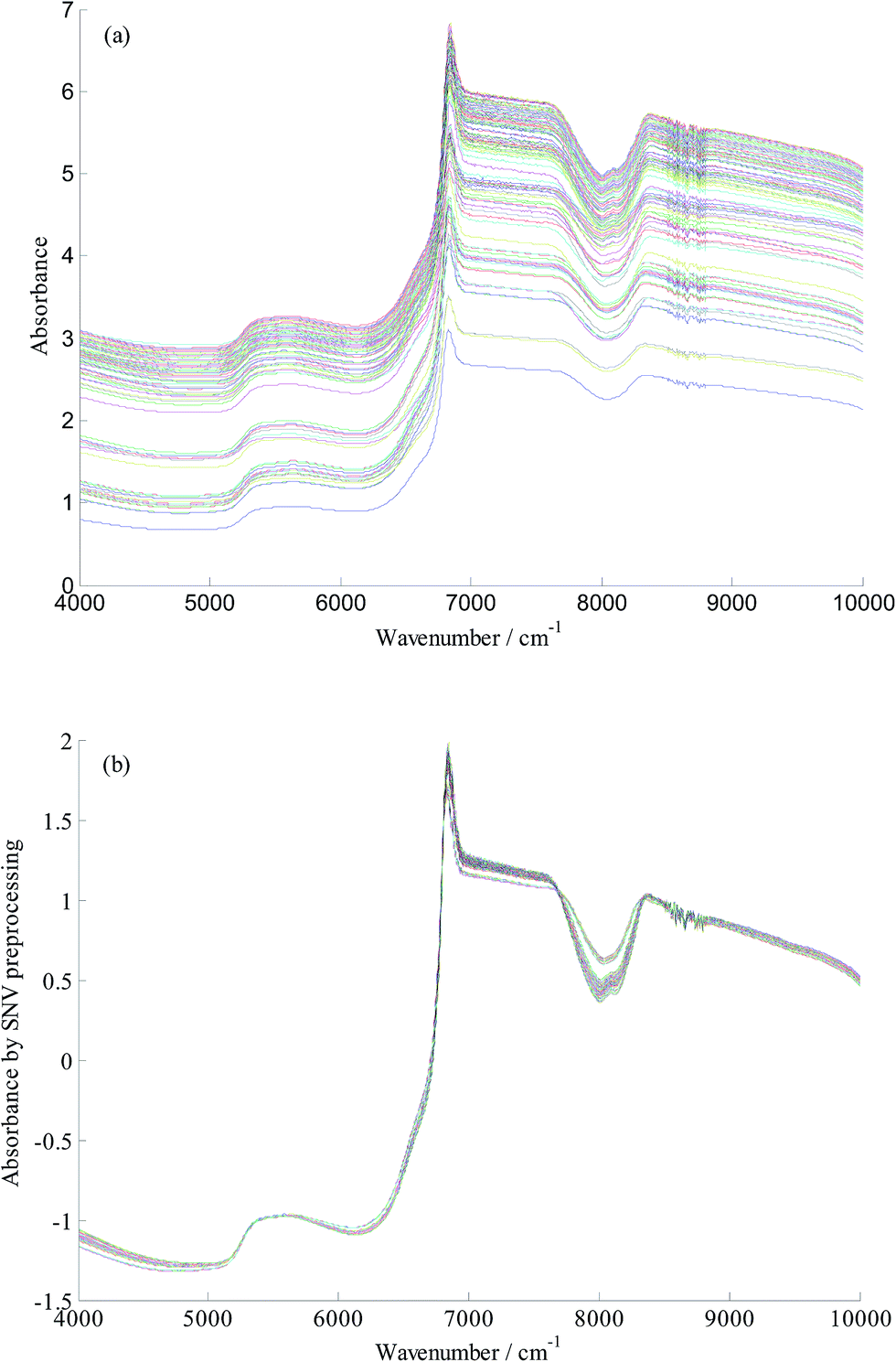 | ||
| Fig. 1 Raw spectra (a) and SNV preprocessing spectra (b) of all the samples. | ||
2.4 Multivariate data analysis
CARS can work in four successive steps:23
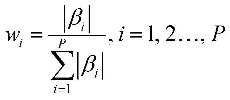
Step 1. Monte Carlo approach was applied for model sampling, 80% of the sample were randomly selected to build the PLS model, and the regression coefficient β of the corresponding model was retained. The weight wi of the ith variable can be defined as follows:
 | (1) |
Step 2. Exponentially decreasing function was employed to perform enforced wavelength selection. Wavelength retention rate was directly calculated using the following algorithm:
| ri = ae−ki | (2) |
Step 3. The adaptive reweighted sampling (ARS) method was adopted to realize a competitive selection of wavelengths. Wavelength variables of the larger weights were selected to form subsets of wavelengths. After repeating this step for N times, CARS sequentially selected N subsets of wavelengths to build the PLS model.
Step 4. 5-Fold cross validation method was utilized to evaluate the subset. The subset with lowest RMSECV value was chosen as the optimal subset.
 | (3) |
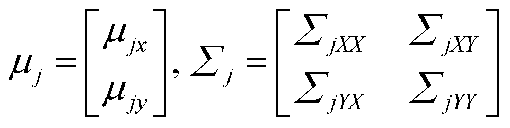
In addition, mean and covariance can be divided into input and output parts as follows:
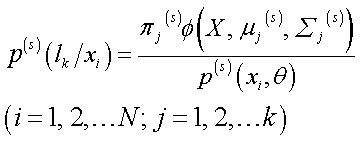
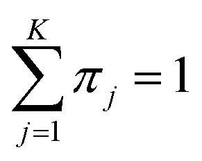 (0 ≤ πj ≤ 1).
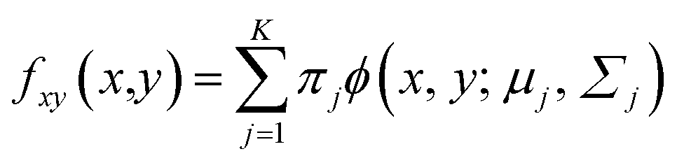
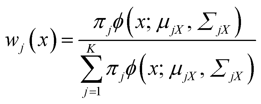
The marginal probability density fX(x) and mixing weight wj(x) can be calculated by27
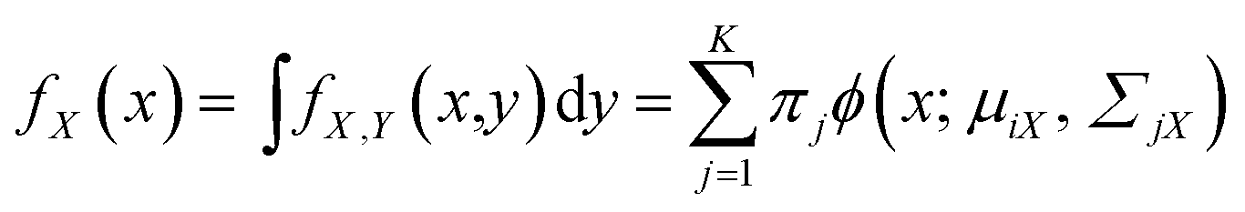 | (4) |
 | (5) |
From eqn (3)–(5), we can obtain the global GMR function as
 | (6) |
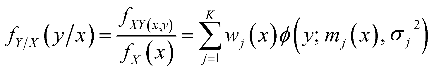
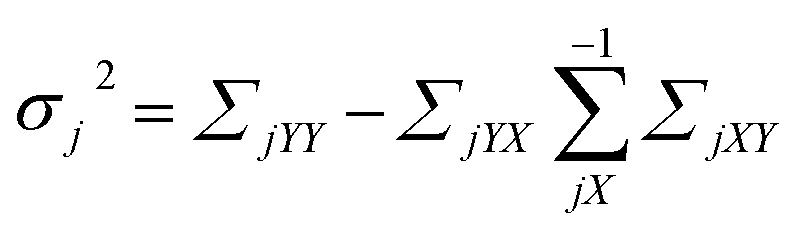
The mean and variance of the conditional distribution can be estimated as follows:
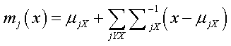 | (7) |
 | (8) |
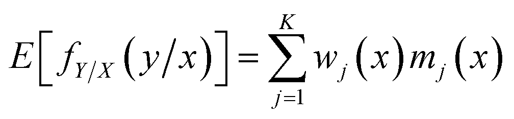
For a given input variable, its prediction can be achieved by calculating the expectation over the conditional distribution fY/X(y/x)27
 | (9) |
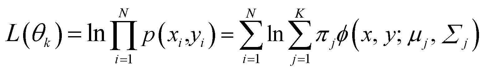
To build a GMM, the mixture components K were set as 4 and the unknown parameter set θ of probabilistic weights were estimated first. Therefore, the maximum likelihood estimation (MLE) and expectation-maximization (EM) algorithm were adopted to optimize the parameters. With a set of given data, (X, Y) can be realized by estimating the model parameters θ in eqn (3). By maximizing the log-likelihood function L(θk), this process can be can realized, and the calculation formula can be expressed as28
 | (10) |
For the given training data, θ was calculated by maximizing this function via the ELM algorithm in the iterative means. It included two steps:29
(1) E step (expectation step):
 | (11) |
(2) M step (maximum step):
 | (12) |
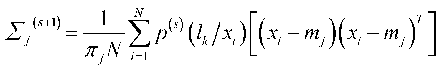 | (13) |
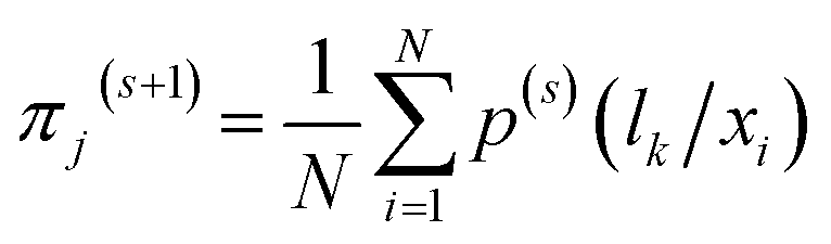 | (14) |
2.5 Software
All the algorithms were implemented in Matlab R2012a (Mathworks, Natick, USA) on Windows 7. The GMR matlab codes were downloaded from http://www.pudn.com/ for free of charge.3. Results and discussion
3.1 Efficient variable selection by CARS
Before model calibration, efficient variables were selected first by CARS algorithm for a simplified model and improving the precision. In the calculations of CARS, the number of Monte Carlo sampling runs was 50, the maximum number of latent variables to be extracted, and the group number for the K-fold cross validation were all set at 5. The data processing method was selected as center.Fig. 2(a) shows the process of the characteristic wavelength selection by CARS. It can be seen from the graph of the relationship between the number of reserved wavelengths and the number of sampling runs that with the increase in the number of runs, the selected wavelength variables present a decreasing trend. This trend was initially rapid and then slowed down, thereby reflecting the process of rough and careful selection of variables. Fig. 2(b) shows the variation trend chart of the root mean square error of cross validation (RMSECV), wherein, it can be seen that RMSECV first descends and then ascends. When the number of sampling runs was 28, RMSECV attained the minimum value at 0.1736. After 28th time sampling, some of the relevant variables started to disappear, thereby increasing the RMSECV value. In Fig. 2(c), “*” perpendicular to the horizontal axis indicates that the minimum value of RMSECV was obtained on 28th time sampling. According to the principle of minimum RMSECV, 13 characteristic variables were selected at last. Fig. 3 shows the distribution of the 13 selected characteristic variables in the entire spectral region after the CARS operation.
 | ||
| Fig. 2 The diagram of CARS variable selecting process. | ||
 | ||
| Fig. 3 Distribution of variables (shown by ‘*’) chosen by the CARS method. | ||
3.2 GMR modeling and prediction results
The GMR algorithm was employed to build a validation mode using the 13 selected characteristic variables by CARS for quantitative analysis. The capabilities of each GMR model were evaluated according to the coefficients of determination (Rp2) and the root mean square error of prediction (RMSEP) in the validation set. GMR model was developed using the selected characteristic variables by CARS algorithm. Fig. 4 shows the prediction effect of GMR model, the prediction is expressed as mean with 2* std (std, standard deviation) error bars (black dotted lines). The regions between the two black dotted lines depict the confidence intervals. In Fig. 4, the red line was found to be very close to the blue line, and the confidence intervals were very small. All these phenomena demonstrated the modeling ability of GMR. The value of RMSEP of GMR model was 0.07262 and Rp2 was 0.98842 in the validation set.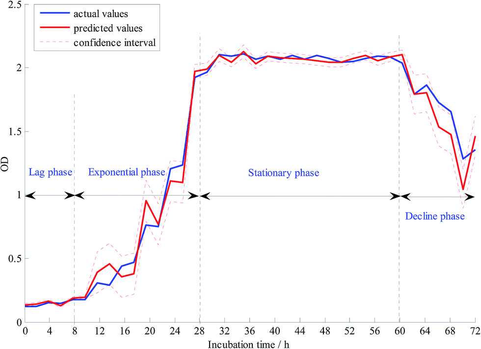 | ||
| Fig. 4 Prediction of the yeast growth process using the GMR model. | ||
3.3 Comparison of different models
To show that GMR has a better predictive performance, it was compared with KPLS, SVR, and ELM approaches in the present study. Table 2 shows the best predicted results obtained via KPLS, SVR, ELM, and GMR approaches in the validation set. As shown in Table 2, the RMSEP of GMR and the operation time of the program were less than those of other models, and Rp2 was found to be higher than that of other models. These results implied that the GMR algorithm has a good generalization performance in model calibration, and another advantage of GMR is that it not only provides accurate prediction results, but also the confidence interval of the results obtained.In addition, through the comparison of these methods, we found that there are several explanations for this phenomenon. KPLS and SVR are the common techniques for the regression of complex non-linear data sets. The key to this model is to map the data in a higher dimensional feature space using kernel transformation. However, the disadvantage of using this kernel function is that the correlation between the obtained regression model and the original input space is lost. As a result, it may lose some useful information variables, which would cause decline in the prediction precision of the model. Moreover, because of the application of the kernel function, the running time KPLS and SVR program is longer than that of other models. ELM as compared to traditional neural network methods has simple structure, high learning speed, and good generalization performance; however, the dimension of the spectral data is usually very high while more hidden nodes should be incorporated in the original ELM model for spectral data. Therefore, the output matrix of the hidden layer of ELM model appeared as a high dimensional and high collinearity problem due to yeast growth in a complex environment. The process data did not originate from a single operating region; moreover, data distribution may be complicated with arbitrary non-Gaussian patterns. As a mixture model can represent arbitrarily complex probability density functions, GMR is one of the ideal tools for modeling complex multi-class dataset. Moreover, GMR not only has the tight structure of a parametric model, but also still retains the flexibility of a nonparametric model. Considering sufficient linear combinations of basis single multivariate Gaussian distribution, GMM can smoothen the probability distribution of arbitrary shape. Therefore, GMR reflected excellent generalization in its theory, which brings a slightly better prediction effect than the other regression algorithms.
4. Conclusions
In this study, a Gaussian mixture regression model based on FT-NIR spectroscopy technique was constructed for quality prediction in the growth progress of yeast. To improve the GMR model fitting, SNV was first used to preprocess the spectra data, and then, the characteristic variables were extracted by the CARS approach. Compared to other conventionally used quantitative analysis approaches (KPLS, SVR, and ELM), GMR exhibited faster computation speed and higher generalization performance.This study not only broadens the scope of CARS and GMR algorithm's application, but also provides a new theoretical basis for the rapid and non-destructive detection of microbial growth process. Moreover, it also makes a reference in the research on the improvement of the fermentation technology informationization and intelligent monitoring of other fermentation processes and has broad application prospect.
Acknowledgements
The authors gratefully acknowledge the financial support provided by the Natural Science Foundation of Jiangsu Province (Grant No. BK20140538, BK20130531, BK20151345), the China Postdoctoral Science Foundation (Grant No. 2016M600381, 2016M601741), the Postdoctoral Science Foundation of Jiangsu Province (Grant No. 1601038C, 1601130B), the College Science Foundation of Jiangsu Province (Grant No. 16KJB210003), the Priority Academic Program Development of Jiangsu Higher Education Institutions (PAPD), the Graduate practical innovation Foundation of Jiangsu province (Grant No. SJZZ16_0193), and the Undergraduate Scientific research Foundation of Jiangsu University (Grant No. 15A137). We would also like to thank many of our colleagues for many stimulating discussions in this field.References
- J. Yu, Z. Xu and T. Tan, Fuel Process. Technol., 2008, 89, 1056–1059 CrossRef CAS.
- J. M. Sablayrolles, A. Pandey, L. V. Rao and C. R. Soccol, Food Res. Int., 2009, 42, 418–424 CrossRef CAS.
- J. B. Doran, J. Cripe, M. Sutton and B. Foster, Appl. Biochem. Biotechnol., 2000, 84–86, 141–152 CrossRef CAS PubMed.
- Y. J. Wu, Y. Jin, Y. R. Li, D. Sun, X. S. Liu and Y. Chen, Vib. Spectrosc., 2012, 58, 109–118 CrossRef CAS.
- Q. S. Chen, J. R. Cai, X. M. Wan and J. W. Zhao, LWT–Food Sci. Technol., 2011, 44, 2053–2058 CrossRef CAS.
- H. Jiang, G. H. Liu, C. L. Mei and Q. S. Chen, Anal. Methods, 2013, 5, 1872–1880 RSC.
- E. D. Louw and K. I. Theron, Postharvest Biol. Technol., 2010, 58, 176–184 CrossRef.
- M. Blanco, A. C. Peinado and J. Mas, Biotechnol. Bioeng., 2004, 88, 536–542 CrossRef CAS PubMed.
- B. Finn, L. M. Harvey and B. Mcneil, Yeast, 2006, 23, 507–517 CrossRef CAS PubMed.
- A. X. Yang, J. L. Ding, H. L. Yan and K. Deng, Spectra Anal., 2016, 36, 691–696 CAS.
- M. H. M. Killner, J. J. R. Rohwedder and C. Pasquini, Fuel, 2011, 90, 3268–3273 CrossRef CAS.
- K. Kim, J. M. Lee and I. B. Lee, Chemom. Intell. Lab. Syst., 2005, 79, 22–30 CrossRef CAS.
- S. K. Feng and H. J. Xu, Infrared Technol., 2008, 30, 58–60 Search PubMed.
- X. D. Sun, X. L. Dong, L. J. Cai, Y. Hao, A. G. Ouyang and Y. D. Liu, Sens. Lett., 2012, 10, 506–510 CrossRef CAS.
- G. B. Huang, H. M. Zhou, X. J. Ding and R. Zhang, IEEE Trans. Syst. Man Cybern. Part B Cybern., 2012, 42, 513–529 CrossRef PubMed.
- A. Yeşilova, M. S. Özgökçe, R. Atlıhan, Ş. Polat Yıldız, İ. Karaca and G. Ser, Fresenius Environ. Bull., 2016, 25, 1768–1778 Search PubMed.
- S. Calinon, F. D’halluin, E. Sauser and A. Billard, IEEE Robotics & Automation Magazine, 2010, 17, 44–54 Search PubMed.
- J. W. Choi, S. H. Lee and S. G. Chung, Afr. J. Microbiol. Res., 2012, 6, 4620–4622 Search PubMed.
- M. C. A. Marcelo, C. A. Martins, D. Pozebon and M. F. Ferrão, Anal. Methods, 2014, 6, 7621–7627 RSC.
- H. L. Zhang and Y. He, Spectra Anal., 2016, 36, 91–95 CAS.
- W. Fan, Y. Shan, G. Y. Li, H. Y. Lv, H. D. Li and Y. Z. Liang, Food Anal. Method, 2012, 5, 585–590 CrossRef.
- C. Xie, X. Ning, Y. Shao and Y. He, Spectrochim. Acta, Part A, 2015, 149, 971–977 CrossRef CAS PubMed.
- H. Li, Y. Liang, Q. Xu and D. Cao, Anal. Chim. Acta, 2009, 648, 77–84 CrossRef CAS PubMed.
- X. F. Yuan, Z. Q. Ge and Z. H. Song, Chemom. Intell. Lab. Syst., 2014, 138, 97–109 CrossRef CAS.
- N. Abramson, D. Braverman and G. Sebestyen, IEEE Trans. Inf. Theory, 1963, 9, 257–261 CrossRef.
- S. Calinon, F. Guenter and A. Billard, IEEE Trans. Syst. Man Cybern. Part B Cybern., 2007, 37, 286–298 CrossRef.
- J. Q. Shi, R. Murray-Smith and D. M. Titterington, Int. J. Adapt. Control Sig. Process., 2012, 17, 149–161 CrossRef.
- B. Muthén and K. Shedden, Biometrics, 1999, 55, 463–469 CrossRef.
- C. L. Mei, Y. Su, G. H. Liu, Y. H. Ding and Z. L. Liao, Chin. J. Chem. Eng., 2017, 25, 116–122 CrossRef CAS.
| This journal is © The Royal Society of Chemistry 2017 |