DOI:
10.1039/D4SM00095A
(Paper)
Soft Matter, 2024,
20, 3845-3853
Spontaneous oscillation of an active filament under viscosity gradients†
Received
22nd January 2024
, Accepted 8th April 2024
First published on 23rd April 2024
Abstract
We investigate the effects of uniform viscosity gradients on the spontaneous oscillations of an elastic, active filament in viscous fluids. Combining numerical simulations and linear stability analysis, we demonstrate that a viscosity gradient increasing from the filament's base to tip destabilises the system, facilitating its self-oscillation. This effect is elucidated through a reduced-order model, highlighting the delicate balance between destabilising active forces and stabilising viscous forces. Additionally, we reveal that while a perpendicular viscosity gradient to the filament's orientation minimally affects instability, it induces asymmetric ciliary beating, thus generating a net flow along the gradient. Our findings offer new insights into the complex behaviours of biological and artificial filaments in complex fluid environments, contributing to the broader understanding of filament dynamics in heterogeneous viscous media.
1 Introduction
Motile cilia, or interchangeably, flagella, are hair-like, flexible filaments protruding from a wide range of cells. Their oscillatory motion facilitates various biological processes, such as propulsion of flagellated algae that can capture CO21,2 and that of planktonic ciliates important in aquatic ecosystems,3 and feeding of marine invertebrates. In mammals,4 flagellar movement is essential for sperm locomotion, while ciliary beating in the airways helps expel mucus and is crucial for transporting oocytes and embryos in the oviduct. Ciliary dysfunction in humans causes up to 35 diseases known as ciliopathies5 including male infertility owing to weakened sperm motility, female infertility due to impaired oviductal cilia, and chronic bronchitis resulting from defective clearance of respiratory mucus. Besides its biological significance, the behaviour of ciliary beating has inspired the design of active filamentous structures for applications in adaptive materials, microfluidics, and drug delivery.6–9
Motivated by its fundamental importance and broad application prospects, a substantial amount of research has been dedicated to examining ciliary oscillation in diverse contexts.10 It is established that a biological filament oscillates spontaneously, typically driven by its internal structure—the central axoneme comprising microtubule doublets and dynein molecular motors. A variety of models have been proposed to elucidate the mechanisms of how dynein motors power spontaneous ciliary oscillation.11–22 Despite these efforts to achieve mechanistic understanding, the proposed models have also facilitated the investigation on synchronisation of two active filaments23–25 and the emergence of metachronal waves generated by multiple filaments,26,27 focusing on inter-filament interactions. More recently, motivated by the typically non-Newtonian bodily fluids hosting cilia and flagella, research has been conducted on a spontaneously oscillating filament in viscoelastic28 or shear-thinning/thickening fluids.29
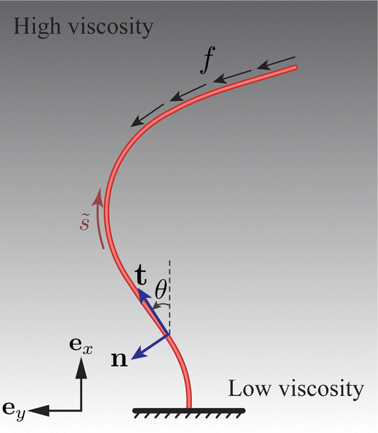
Besides these recognised rheological complexities, heterogeneity is also a notable characteristic in bodily fluids, often manifesting as spatially varying viscosity. A key question is how will the viscosity gradient affect ciliary oscillation? In this work, we will address this question, but before that, let us mention the biological relevance of this scenario. It is relevant to the beating of pulmonary cilia in the airway surface liquid (ASL) that is essential for mucociliary clearance. Overlaying the airway epithelium, the ASL comprises two distinct layers: a gel-like mucus layer above a periciliary layer (PCL), as depicted in Fig. 1.
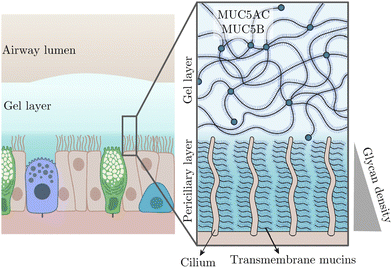 |
| | Fig. 1 Schematic of pulmonary cilia in the airway surface liquid adapted from ref. 30 with permission from Elsevier. This liquid consists of a more viscous gel layer on top of a less viscous periciliary layer (PCL). The PCL approximately contains the cilia and features a growing density of glycan from top to bottom, thus leading to a viscosity gradient. | |
Both layers contain mucins—large macromolecules forming networks31—but differ in their types and, consequently, in fluid viscosities; the PCL is less viscous than the superficial gel layer. In addition to such a viscosity patchiness in the ASL, the PCL—typically as deep as cilia, presents its own viscosity heterogeneity. Specifically, the cilia immersed in the PCL are rich in transmembrane mucins, producing a glycan meshwork with a density that increases towards the airway surface.30 This density gradient, in turn, results in a viscosity variation parallel to the ciliary orientation.
Inspired by the picture depicted above, this study explores the spontaneous oscillation of an active elastic filament in viscous fluids exhibiting viscosity heterogeneity. Simulations are conducted in the creeping flow regime to examine the influence of uniform viscosity gradients on the emergence of oscillatory instability. These numerical findings are corroborated by stability analysis. We then employ a reduced-order model to further clarify the underlying mechanisms by which viscosity gradients affect the instability.
2 Problem setup
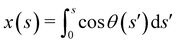
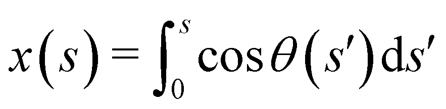
We consider a slender, inextensible filament undergoing spontaneous oscillation in a quiescent creeping flow of Newtonian fluid with spatially varying viscosity. The filament of length L features a circular cross-section with diameter b ≪ L, leading to a vanishing slenderness β = b/L ≪ 1. Its profile is described by the centerline coordinates ![[r with combining tilde]](https://www.rsc.org/images/entities/b_char_0072_0303.gif) (
(![[s with combining tilde]](https://www.rsc.org/images/entities/i_char_0073_0303.gif) ,
, ![[t with combining tilde]](https://www.rsc.org/images/entities/i_char_0074_0303.gif) ) as functions of arc length ∈ [0, L] and time . From hereinafter, dimensional variables (but not constant values) are indicated by a tilde.
) as functions of arc length ∈ [0, L] and time . From hereinafter, dimensional variables (but not constant values) are indicated by a tilde.
The filament is vertically clamped at its base ( = 0) and, in its undeformed, relaxed state, aligns along the vertical (ex) direction (see Fig. 2). To emulate the active force exerted by the molecular motors, we employ the follower force approach,17,32 applying a compressive force density uniformly distributed along the filament centerline, aligned with its tangent everywhere. For a related configuration featuring a point follower force of constant magnitude at the tip ( = L), the results, exhibiting trends similar to those for the distributed force, are given in the ESI.† A sufficiently strong follower force or force density can induce the filament to self-oscillate, simultaneously driving the surrounding flow.20,32,33
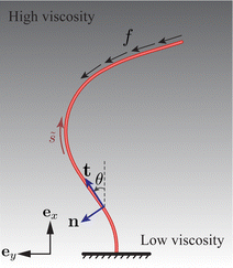 |
| | Fig. 2 Schematic of an elastic filament submerged in a fluid with a vertical viscosity gradient. The filament is anchored at one end and free at its tip. Its shape is characterised by the tangent angle θ(, ), where represents the arc length. The local tangent and normal vectors are denoted as t(, ) and n(, ), respectively. The filament experiences a distributed active force with density −ft along its centerline. | |
The motion of the filament is restricted to the xy plane, see Fig. 2. Consequently, its profile remains planar, and is determined by the angle θ(, ) between the tangent vector t(, ) = cos![[thin space (1/6-em)]](https://www.rsc.org/images/entities/char_2009.gif) θex + sinθey and the ex axis. The associated normal vector is n(, ) = −sinθex + cosθey.
θex + sinθey and the ex axis. The associated normal vector is n(, ) = −sinθex + cosθey.
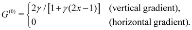
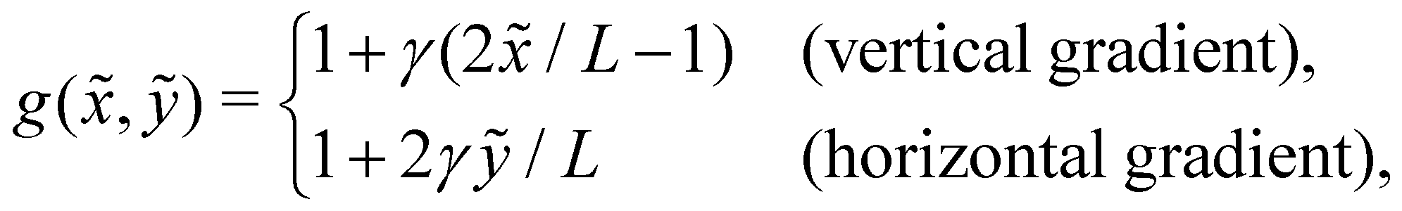
To probe the influence of the viscosity gradient, we prescribe a viscosity ![[small mu, Greek, tilde]](https://www.rsc.org/images/entities/i_char_e0e0.gif) (
(![[x with combining tilde]](https://www.rsc.org/images/entities/i_char_0078_0303.gif) , ỹ) linearly changing in one direction—either vertically (ex) or horizontally (ey). Choosing a reference viscosity μ0 measured at the middle (L/2,0)ỹ of the undeformed filament, we express the viscosity as (, ỹ) = μ0g(, ỹ). Hence, g(, ỹ) represents a scaled viscosity profile, which features two forms depending on the viscosity gradient direction:
, ỹ) linearly changing in one direction—either vertically (ex) or horizontally (ey). Choosing a reference viscosity μ0 measured at the middle (L/2,0)ỹ of the undeformed filament, we express the viscosity as (, ỹ) = μ0g(, ỹ). Hence, g(, ỹ) represents a scaled viscosity profile, which features two forms depending on the viscosity gradient direction:
| | 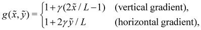 | (1) |
where
γ signifies a dimensionless viscosity gradient magnitude.
3 Elasto-hydrodynamics at a low Reynolds number
Here, we describe the low-Reynolds-number elasto-hydrodynamics in the Stokes flow limit. Instantaneous balance between the active force, elastic force, and hydrodynamic force holds everywhere on the filament centerline. The active force density (per unit length) −ft, imposed anti-parallel to the tangent vector t, possesses a constant magnitude f. The internal elastic force density ![[f with combining tilde]](https://www.rsc.org/images/entities/b_char_0066_0303.gif) e =
e = ![[small tau, Greek, tilde]](https://www.rsc.org/images/entities/i_char_e0e5.gif) t + Ñn consists of a tangential tension component and a normal component Ñ = −Aθ, where A is the bending modulus of the filament (see the ESI,† Section S1) and the subscript denotes differentiation with respect to the arc-length.
t + Ñn consists of a tangential tension component and a normal component Ñ = −Aθ, where A is the bending modulus of the filament (see the ESI,† Section S1) and the subscript denotes differentiation with respect to the arc-length.
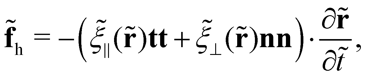
The hydrodynamic force on slender filaments in Stokesian fluids with a constant viscosity is typically addressed using the resistive force theory—the leading order slender-body theory.34–38 Kamal and Lauga39 recently extended the classical theories to incorporate a constant viscosity gradient in fluids. At the leading order of filament slenderness β, the hydrodynamic force aligns with the classical theories for fluids with a uniform viscosity, except that the viscosity everywhere takes its locally non-constant value. At the next order of β, non-local terms emerge. Here, we address solely the leading-order effects, and consequently, the hydrodynamic force density reads
| |  | (2) |
where
![[small xi, Greek, tilde]](https://www.rsc.org/images/entities/i_char_e119.gif) ⊥
⊥(
) and
‖(
) denote the viscous resistance coefficients that linearly scale with the local viscosity
(
) measured at
(
). Based on this linear relationship, we obtain
⊥(
,
ỹ) =
g(
,
ỹ)
ξ⊥,0 and
‖(
,
ỹ) =
g(
,
ỹ)
ξ‖,0. Here,
ξ⊥,0 = 4π
μ0/(−ln
β + 1/2) indicates the resistance coefficient defined at the reference position (
L/2,0)
ỹ, and
ξ⊥,0/
ξ‖,0 = 2 as we take the limit of
β → 0 throughout this study. Accordingly,
⊥(
,
ỹ)/
‖(
,
ỹ) = 2.
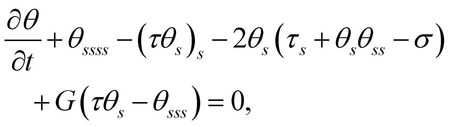
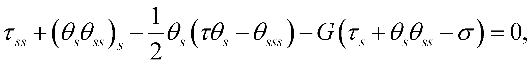
4 Governing equations and nondimensionalisation
The equations governing the dynamics of the filament can be derived by imposing force and torque balances along the filament, as elaborated in Section S1 of the ESI.†
Scaling forces with A/L2, lengths with L, and time with ξ⊥,0L4/A, we obtain the following dimensionless governing equations:
| | 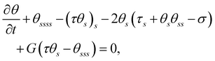 | (3a) |
| |  | (3b) |
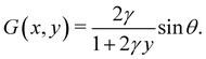
where
G(
x,
y) =
gs/
g indicates the relative change of viscosity over the filament arc length, and
σ =
fL3/
A represents the dimensionless active force scaled by elastic forces. In the absence of viscosity gradients,
G = 0,
eqn (3) recovers to the governing equations in ref.
33. Imposing a vertical viscosity gradient defined in
eqn (1),
| |  | (4) |
where we have employed
to compute ∂
x/∂
s. Similarly, for a horizontal viscosity gradient, we derive
| |  | (5) |
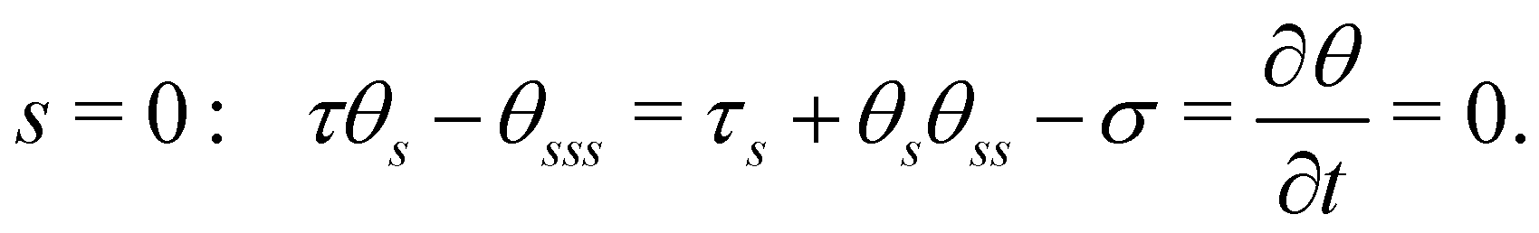
Eqn (3) is solved with boundary conditions (BCs). At the filament tip (s = 1), force- and torque-free conditions hold, corresponding to:
| | | s = 1: τ = θs = θss = 0. | (6) |
At the clamped end (
s = 0), the BCs are:
| | 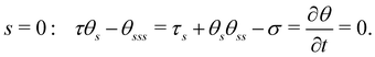 | (7) |
We adopt a Chebyshev spectral method to discretize the governing equations in space, combining an implicit–explicit temporal scheme, as detailed in Section S2 of the ESI.†
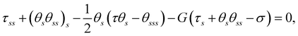
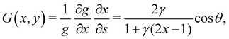
5 Linearisation of the governing equations
Subject to a sufficient small active force, the filament maintains a stationary and straight equilibrium state. To investigate its stability, we linearise the governing equations eqn (3) around this equilibrium. Assuming small filament deformation, we adopt a linear expansion: θ = θ(0) + εθ(1)(s, t) and τ = τ(0)(s) + ετ(1)(s, t), where (θ(0), τ(0)) and (θ(1), τ(1)) denote the zero-th and first order solutions, respectively, with ε ≪ 1 being a small parameter.
Upon linearisation, we obtain θ(0) = 0 and
| | | τ(0)ss − G(0)(τ(0)s − σ) = 0, | (8) |
with
| |  | (9) |
From
eqn (8) and the BCs, we obtain
τ(0) =
σ(
s − 1).
Knowing the base state, we derive the governing equation for θ(1),
| |  | (10) |
where
θ(1) and
τ(1) have been decoupled. Considering
eqn (9) and (10) together, we recognise that the horizontal viscosity gradient does not affect the linear stability because of the vanishing
G(0), but only the vertical gradient does.
The linearised BCs for θ(1) are:
| |  | (11a) |
| | | s = 1: θ(1)s = θ(1)ss = 0. | (11b) |
Employing the normal form
θ(1)(
s,
t) =
![[small straight theta, Greek, circumflex]](https://www.rsc.org/images/entities/i_char_e12d.gif)
(
s)exp(
ωt) with
ω the complex growth rate, we arrive at a classical eigenvalue problem,
| | | ω + ssss − σs − σ(s − 1)ss + G(0)[σ(s − 1)s − sss] = 0. | (12) |
The leading (most unstable) eigenvalue and its associated eigenmode can be obtained by numerically solving
eqn (12) using the same spectral discretization as for solving
eqn (3), see the ESI,
† Section S2.
6 Results: nonlinear simulations and linear stability analysis
We numerically solve eqn (3) to examine the effect of viscosity gradient on the spontaneous filament oscillation, particularly focusing on the instability threshold. These nonlinear simulations are corroborated by linear stability analysis (LSA). We then employ a reduced-order bead-spring model to seek deeper insights into the instability mechanism modulated by the viscosity gradient. The effects of vertical and horizontal viscosity gradients will be demonstrated separately below, starting from the former.
6.1 Filament in a vertical viscosity gradient
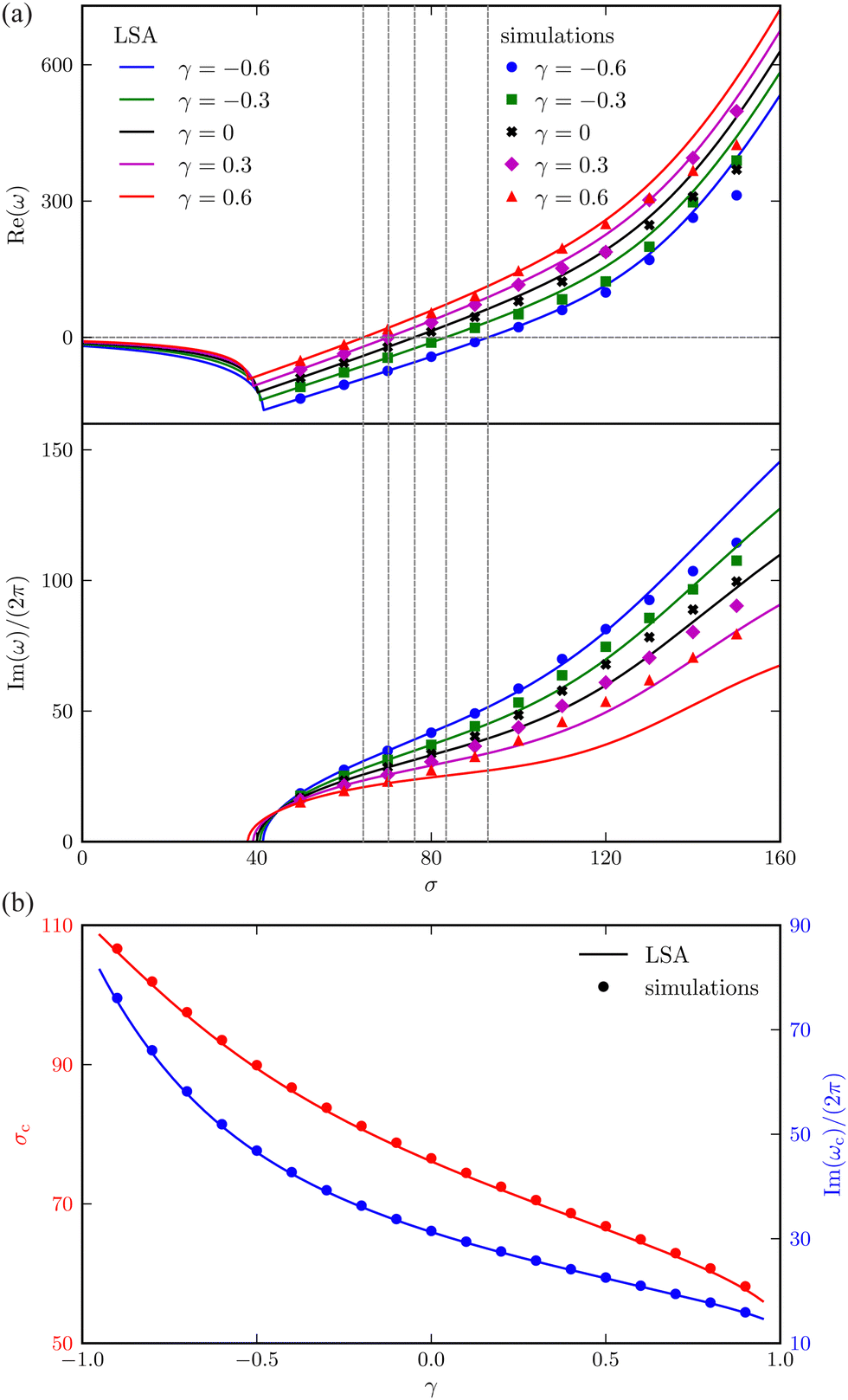
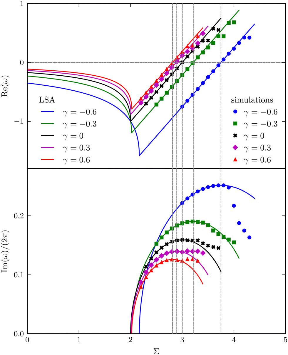
Fig. 3(a) shows how the complex growth rate ω of perturbation depends on the dimensionless active force σ and the vertical viscosity gradient γ ∈ [−0.6, 0.6]. The vertical dashed lines represent the critical active force σc, beyond which spontaneous filament oscillation emerges due to instability. Close to this threshold, the values of σ predicted by LSA and nonlinear simulations show excellent agreement.
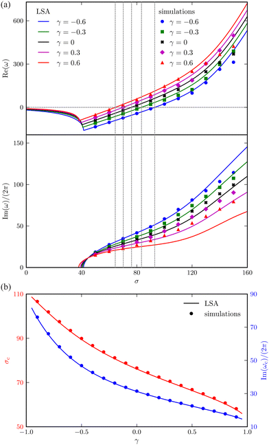 |
| | Fig. 3 Comparison between the LSA (lines) and numerical results (symbols) for an active filament. (a) The real part (growth rate of the perturbation) of the most unstable eigenvalues, and corresponding frequency of oscillation (imaginary part divided by 2π), versus the dimensionless active force σ for different γ. The vertical dashed lines indicate the critical σc corresponding to the onset of instability. (b) Critical σc and oscillation frequency Im(ωc)/(2π) as a function of γ. | |
More importantly, a negative correlation between the instability threshold σc and the gradient γ is clearly observed. This trend is further revealed in Fig. 3(b), showing that both σc and the frequency of the corresponding most unstable eigenmode Im(ωc)/2π at the onset decrease with γ monotonically. This suggests that a viscosity profile increasing from the base to the tip of the filament destabilises the system, thereby promoting its self-oscillation.
6.2 Filament in a horizontal viscosity gradient
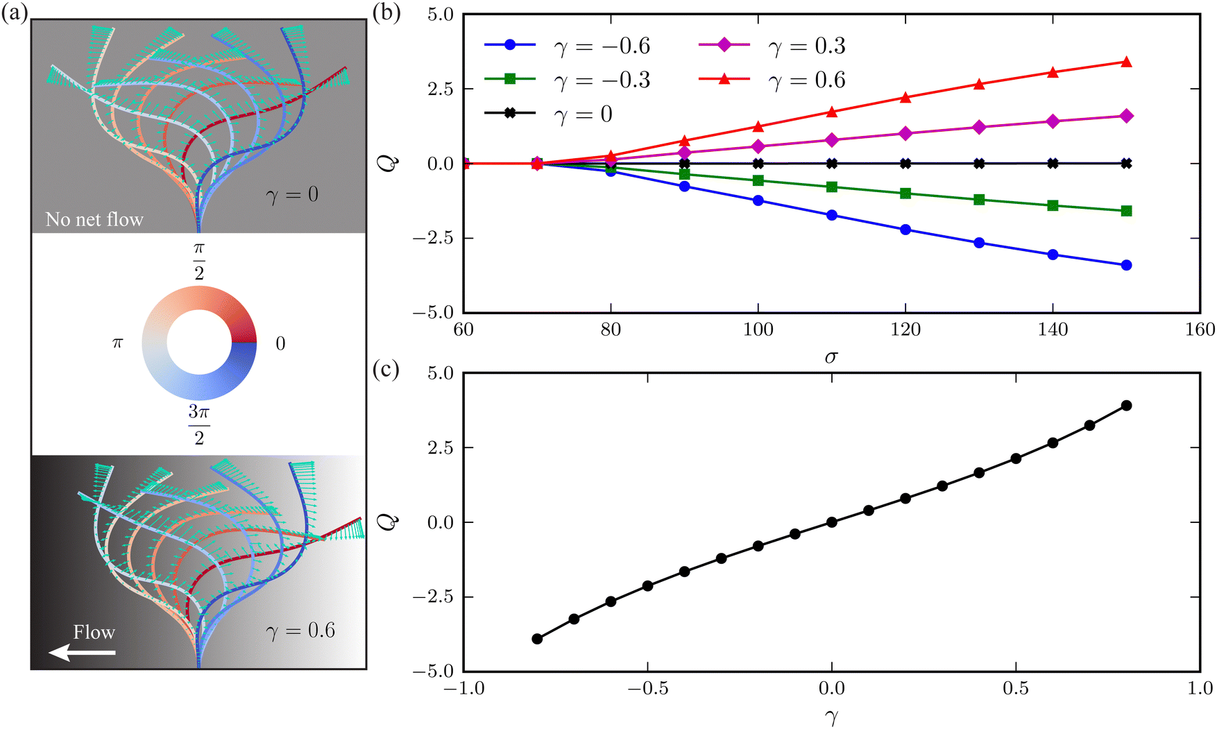
The scenario of linear instability is independent of the horizontal viscosity gradient, as indicated by eqn (9). This independence near the onset of instability is confirmed by the numerically computed ω versus σ (see the ESI,† Section S4). Notably, even when σ substantially exceeds the threshold, the influence of the viscosity gradient on ω remains marginal.
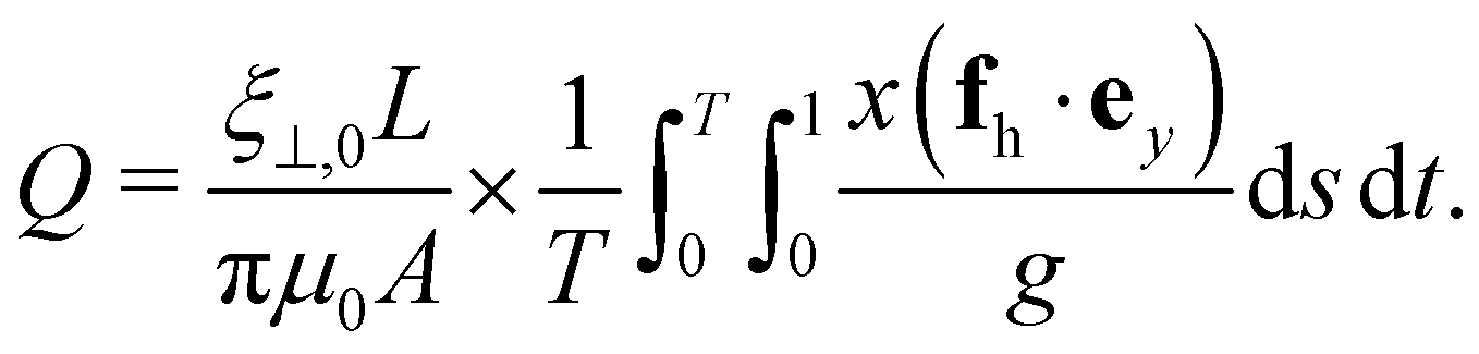
The horizontal viscosity gradient breaks the left-right symmetry in a forced fashion; hence, the filament exhibits asymmetric beating as expected. However, this asymmetry remains mild even at a substantial gradient level of γ = 0.6, as illustrated by the bottom panel of Fig. 4(a). Intuitively, the asymmetric beating resembling the recover-and-stroke pattern of a natural cilium would pump the fluid horizontally. To characterise this pumping effect, we calculate the average volume flow rate over one oscillation period T = 2π/Im(ω):40,41
| | 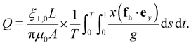 | (13) |
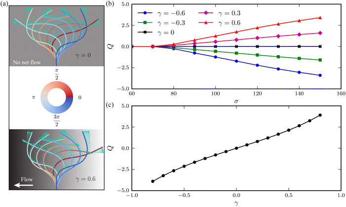 |
| | Fig. 4 (a) Time-lapse of filament waveforms over one beating cycle for two viscosity gradients γ = 0 (top panel) and γ = 0.6 (bottom panel) at a dimensionless active force σ = 130. The black and white background suggests the fluid viscosity, where black corresponds to a higher viscosity. Arrows indicate the instantaneous velocities of the filament's centerline. (b) Average volume flow rate Q versus σ at varying viscosity gradients γ. (c) Dependence of Q on γ when σ = 130. | |
As evidenced in Fig. 4(b), the flow rate Q exhibits an almost linear increase with the dimensionless active force σ above the threshold. The fluid is propagated along the viscosity gradient. Moreover, the net flow rate grows with the viscosity gradient γ, following an approximately linear relationship, as illustrated in Fig. 4(c).
7 Reduced-order model
In the preceding section, we show the significant effect of vertical viscosity gradient on the onset of instability. In this section, we examine this effect further based on a reduced-order minimal model. Similar models have been employed by other studies on the behaviour of flexible structures in viscous fluids.32,42–50
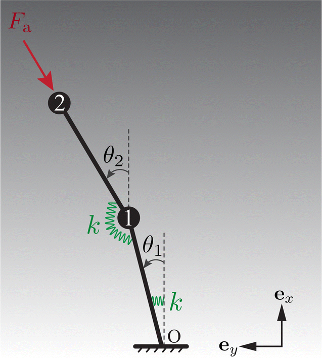
As shown in Fig. 5, this model comprises two beads numbered 1 and 2 sequentially connected to two links of length L/2. Akin to the full model, only planar motion restricted to the xy plane is considered. To incorporate elasticity, the links are joined by a torsional spring of stiffness k. Besides, the lower link is attached to the base using a similar spring. The i-th (i = 1, 2) bead is centred at i. The angles θ1 and θ2 represent the orientation of the lower and upper links, respectively, relative to the ex axis.
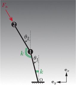 |
| | Fig. 5 The reduced-order model comprises two torsional springs and two beads, encapsulating the minimal physical ingredients of elasto-hydrodynamics: elastic torques generated by the springs and hydrodynamic forces exerted on the moving beads. | |
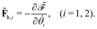
A follower force ![[F with combining tilde]](https://www.rsc.org/images/entities/b_char_0046_0303.gif) a = −Fa(cosθ2, sinθ2) is imposed on bead 2 to represent the active force, persistently opposite to the tangent of the upper link. The hydrodynamic force exerted on bead i takes the form h,i = −
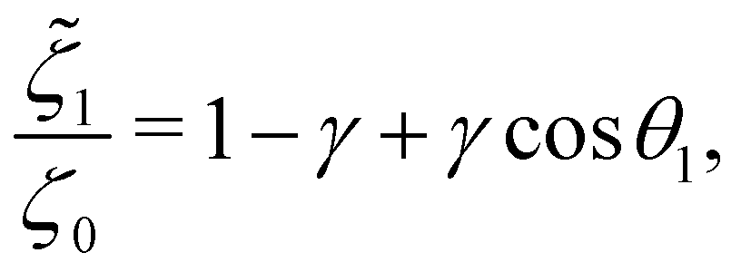
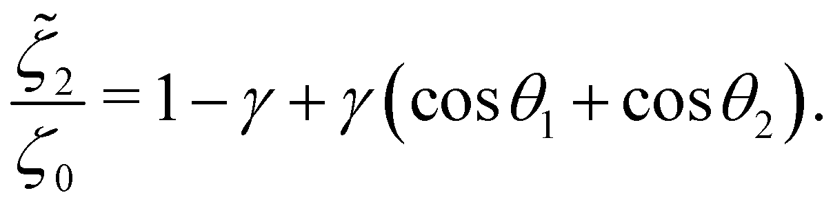
a = −Fa(cosθ2, sinθ2) is imposed on bead 2 to represent the active force, persistently opposite to the tangent of the upper link. The hydrodynamic force exerted on bead i takes the form h,i = −![[small zeta, Greek, tilde]](https://www.rsc.org/images/entities/i_char_e126.gif) i∂i/∂, with i indicating the drag coefficient of bead i. Considering the vertical viscosity gradient, i/ζ0 = 1 + γ(2i·ex/L − 1). Here, ζ0 represents the reference drag coefficient.
i∂i/∂, with i indicating the drag coefficient of bead i. Considering the vertical viscosity gradient, i/ζ0 = 1 + γ(2i·ex/L − 1). Here, ζ0 represents the reference drag coefficient.
Employing the principle of virtual work, or the Euler–Lagrangian equations detailed in the Appendix, we derive the dimensionless governing equations for the reduced-order model:
| |  | (14a) |
| | θ1 − θ2 − [1 − γ + γ(cosθ1 + cosθ2)][![[small theta, Greek, dot above]](https://www.rsc.org/images/entities/i_char_e0a7.gif) 2 + 1cos(θ2 − θ1)] = 0, 2 + 1cos(θ2 − θ1)] = 0, | (14b) |
where
Σ =
FaL/2
k represents the dimensionless active force. Here, we have chosen
ζ0L2/4
k as the characteristic time scale, and the overdot denotes taking a derivative with respect to time. Linearising
eqn (14) about the equilibrium configuration
θ1 =
θ2 = 0, we examine the stability. Using the normal mode approach, we substitute
θ1,2 =
1,2exp(
ωt) in the linearised equation and obtain,
| | | Σ(1 − 2) − 21 + 2 − ω[(2 + γ)1 + (1 + γ)2] = 0, | (15a) |
| | | 1 − 2 − ω(1 + γ)(1 + 2) = 0. | (15b) |
Non-trivial solutions to
eqn (15) exist when the determinant of the system is zero,
i.e., 1 + [6 +
γ(5 − 2
Σ) − 2
Σ]
ω + (1 +
γ)
ω2 = 0, leading to the complex growth rate:
| |  | (16) |
The complex growth rate ω implies five stability regimes depending on Σ and γ:
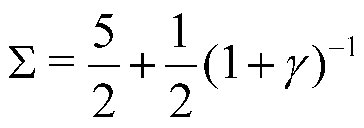
1. Stable, when  :
:
Re(ω±) < 0 and Im(ω±) = 0, corresponding to a stable state.
2. Decaying oscillations, when  :
:
Re(ω±) < 0 and Im(ω±) ≠ 0, indicating decaying oscillations.
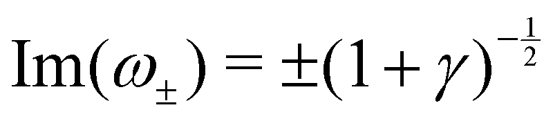
3. Stable periodic oscillations, when 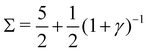 :
:
Re(ω±) = 0 and  , and the system oscillates with a constant amplitude. Besides, increasing γ decreases Σc and the oscillation frequency.
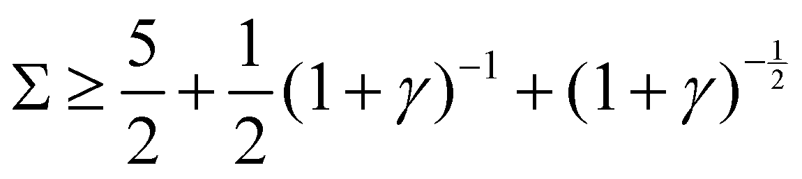
4. Exponentially growing oscillations, when  :
:
Re(ω±) > 0 and Im(ω±) ≠ 0, indicating exponentially growing oscillations.
5. Unstable, when  :
:
Re(ω±) > 0 and Im(ω±) = 0, the amplitude grows without bound, indicating an unstable system that diverges.
As illustrated in Fig. 6, the complex growth rate ω versus Σ and γ reveals the first four regimes discussed above. Moreover, the trend qualitatively agrees with that of the continuum filament model shown in Fig. 3(a). Based on the capacity of the reduced-order model to capture the characteristic behaviours of the full model, we will further exploit the model to understand the physical mechanisms underlying the destabilisation of the vertical viscosity gradient.
 |
| | Fig. 6 Real and imaginary parts of the complex growth rate ω versus the dimensionless active force Σ with varying viscosity gradients γ, obtained from LSA (symbols) and simulations (lines) for the bead-spring model. | |
7.1 Physical mechanisms of destabilising vertical viscosity gradient
Upon applying a vertical viscosity gradient γ > 0, the fluid surrounding bead 2 (upper) becomes more viscous, whereas the viscosity around bead 1 (lower) remains unchanged, because bead 1 stays near its equilibrium state close to the reference position ỹ = L/2. Naturally, we may wonder whether the stabilisation results from an overall viscosity enhancement. Intriguingly, owing to the independence of Σ on the viscosity, increasing the viscosity homogeneously by the same factor (thus eliminating the gradient) does not alter the onset Σc of instability. A uniform viscosity enhancement merely affects the oscillation frequency. Consequently, we deduce that it is the gradient of viscosity, rather than its overall magnitude, that affects the stability, as we will explain below based on an energetic point of view.
In the Stokes flow regime, the energy of the bead-spring system comprises the elastic energy, E, of the springs, because the kinetic energy of the beads vanishes. The temporal growth rate of E is powered by the active force and simultaneously dissipated by the viscous force, namely,
where
Pa denotes the power of active force, and
Pv the viscous dissipation rate. They take the form
| | | Pa = Σsin(θ1 − θ2)1, | (18a) |
| |  | (18b) |
where

is the dissipation function derived in the Appendix. Near the equilibrium where
θ1 ≈
θ2 ≪ 1, they can be approximated by
| | | Pa ≈ (1 + γ)Σ(1 + 2)1, | (19a) |
| | | Pv ≈ 12 + (1 + γ)(1 + 2)2. | (19b) |
Eqn (19) allows us to analyse the linear stability from the energetic perspective. Evidently,
Pv is always positive, indicating the consistent stabilisation due to the viscous dissipation. On the other hand, the active power
Pa can generally switch sign, with
Pa > 0 corresponding to the destabilisation triggered by the active force. Furthermore,
eqn (19) implies that the active force is the only destabiliser in this system, as indeed aligning with the physical intuition.
The viscosity gradient γ affects the stability by modulating the (1 + γ) – dependent Pa and Pv. In both cases, (1 + γ) appears as a prefactor of active force strength Σ in the former, and of a portion of the viscous power in the latter. Hence, a positive gradient γ amplifies both Pa and Pv, whereas a negative γ decreases both.
In the limit of γ → −1, the active power reduces to zero whereas the viscous dissipation rate remains finite. This leads to a stable system, irrespective of the active force strength. This picture delineates the stabilising effect of a decreasing γ, particularly when it approaches its lower limit. However, beyond this limit, eqn (19) fails to explicitly elucidate the consequences of altering γ on the system's power balance and stability. To address this gap, we analyse the numerical data for Σ = 3 at γ = −0.01, 0, and 0.01. Our findings, presented in Fig. 7, depict the impact of varying γ on the temporal evolution of Pa and −Pv, as well as their summation Ė. Notably, increasing γ leads to a more pronounced amplification of the active power Pa compared to the negative viscous dissipation rate −Pv, and concomitantly more intense oscillations in Ė. This observation reflects, semi-phenomenologically, the destabilising effect of a larger γ.
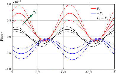 |
| | Fig. 7 Power balance within an oscillation period T of the bead-spring system, when the viscosity gradient γ = 0.01 (dashed lines), γ = 0 (solid lines), and γ = −0.01 (dotted lines) at Σ = 3. Here, Pa (red) and Pv (blue) represent the active power and viscous dissipation rate, respectively. | |
8 Conclusions and discussion
In this work, we have numerically studied the spontaneous oscillation of an anchored active filament in viscous fluids with a linearly varying viscosity. The activity of the filament is modelled by a point follower force or a uniformly distributed force density. In both scenarios, our simulations reveal that a positive viscosity gradient, extending from the filament's base to tip, facilitates its self-oscillation, namely, decreasing the minimum activity required to trigger the elasto-hydrodynamic instability. On the other hand, the viscosity gradient orthogonal to the orientation of the filament does not alter the onset of instability. However, by introducing forced symmetry breaking, this orthogonal gradient enables asymmetric beating of the filament, consequently generating a net fluid pumping along the gradient.
The numerically demonstrated effects of viscosity gradients on the self-oscillatory stability of the active filament are supported by our LSA. Numerical results and predictions of LSA agree excellently near the instability threshold. To better understand how viscosity gradients affect the instability, we have used a reduced-order model. This model reproduces the various stability regimes identified in the original filament model and provides analytical insights into the interplay between the destabilising active force and the stabilising viscous dissipation. Specifically, by increasing the vertical viscosity gradient, we observe an enhanced temporal oscillation in both the active power and the viscous dissipation rate. This enhancement is more pronounced for the former than for the latter, resulting in a more intense oscillation of the elastic energy's growth.
While our study is inspired by respiratory cilia in heterogeneous bodily fluids, it does not delve into the biological implications within this specific context. As a highly complex fluid, ASL is not only heterogeneous and layered,51 but also features viscoelasticity52 and potentially shear-thinning properties.53 The rheological behaviour of ASL is substantially more complex compared to the Newtonian fluid model with uniform viscosity gradient used here. Notably, a similar Newtonian model with spatial viscosity variation has been employed in the investigation of mucociliary clearance enabled by beating cilia.53
To investigate the effects of viscosity gradients on ciliary oscillation, we have employed the simplified follower force approach, which may lack realism. For a deeper, biologically pertinent understanding, future work should explore models of ciliary oscillation driven by dynein motors.11–22
It is worth noting that this study resonates with the recent investigations on microswimmers’ self-propelling in viscous fluids with viscosity gradients.54–61 Consequently, a pertinent inquiry is the behaviour of a spontaneously beating flagellum, with or without a cell body, in environments featuring continuous or sharp viscosity gradients. In the absence of the gradient, a single flagellum is expected to swim along a spontaneously emerging direction depending on its initial orientation. We hypothesise that introducing an external viscosity gradient could direct the flagellum to move along a preferential direction. This hypothesis will be tested in our future studies.
Conflicts of interest
There are no conflicts to declare.
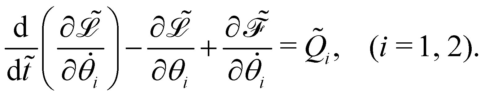
Appendix
Dynamics of the bead-spring system
The governing equations of the bead-spring model are derived based on the Euler–Lagrangian framework:62| |  | (20) |
Here,  represents the Lagrangian of the system
  where
where ![[T with combining tilde]](https://www.rsc.org/images/entities/i_char_0054_0303.gif) kin and Ṽ denote the kinetic and potential energies, respectively. The generalised forces
kin and Ṽ denote the kinetic and potential energies, respectively. The generalised forces ![[Q with combining tilde]](https://www.rsc.org/images/entities/i_char_0051_0303.gif) i are expressed as:
i are expressed as:| |  | (21) |
where the follower force a can be regarded as an external force of the system.
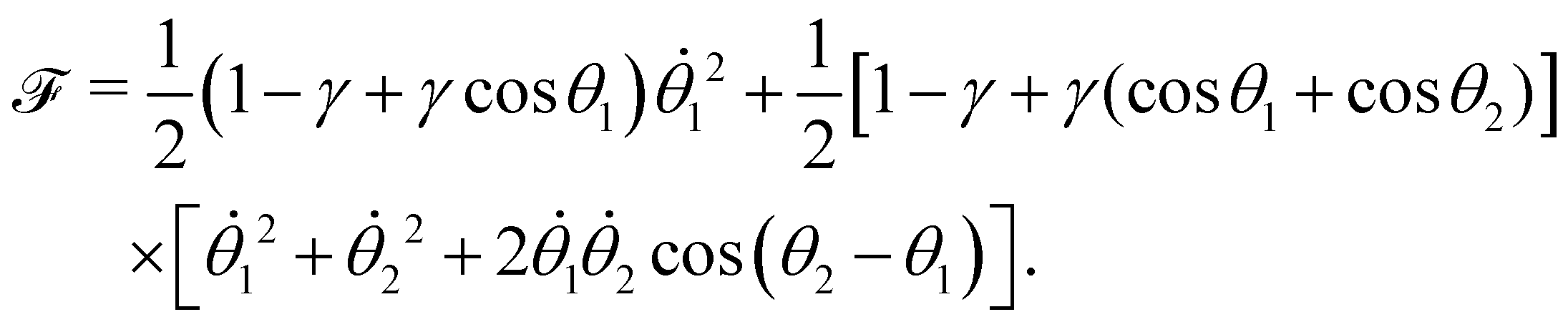
The dissipation function  corresponding to eqn (20) is defined as62
| |  | (22) |
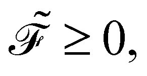
This function remains non-negative, namely,

offers two physical interpretations. Firstly, it represents the velocity-dependent potential, wherein the hydrodynamic force can be computed as
| |  | (23) |
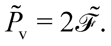
Secondly, it characterises the rate of total energy dissipation, specifically, the viscous dissipation rate
![[P with combining tilde]](https://www.rsc.org/images/entities/i_char_0050_0303.gif) v
v in this system,
| |  | (24) |
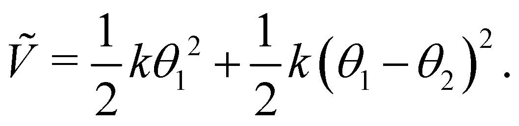
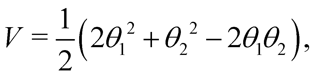
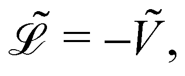
Because the bead mass is neglected, the total kinetic energy of the system is zero, kin = 0. Hence,  with the potential energy Ṽ written as:
| | 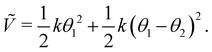 | (25) |
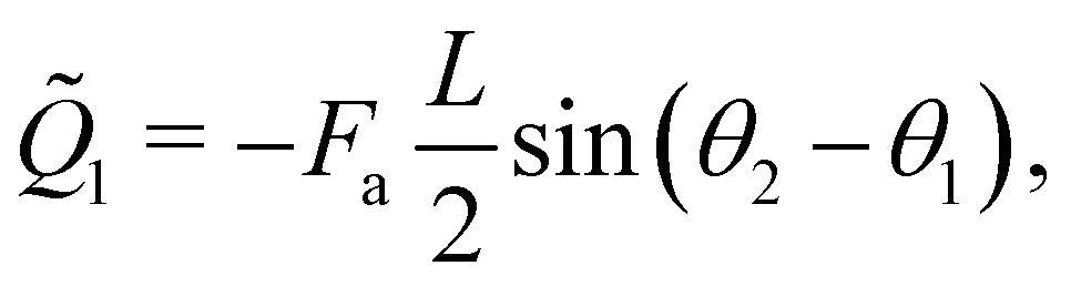
Besides, the two generalised forces corresponding to
θ1 and
θ2 are
| |  | (26a) |
| | | 2 = 0. | (26b) |
In addition, the drag coefficients of both beads under the viscosity gradient are:
| | 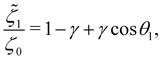 | (27a) |
| | 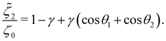 | (27b) |
Choosing k, 2k/L, and ζ0L2/4k as the characteristic energy, force, and time, respectively, the dimensionless potential energy, generalised force, and dissipation function are given as follows:
| |  | (28a) |
| | | Q1 = Σsin(θ1 − θ2), | (28b) |
| |  | (28c) |
By substituting eqn (28) into the dimensionless equation of eqn (20), we obtain eqn (14). The rate of work done by the follower force is
| | | Pa = Fa·ṙ2 = Q11 = Σsin(θ1 − θ2)1. | (29) |
Acknowledgements
The work is funded by the Singapore Ministry of Education Academic Research Fund Tier 2 grant (MOE-T2EP50122-0015). L. Z. acknowledges the partial support from the Paris-NUS joint research grant (ANR-18-IDEX-0001 & A-0009528-01-00). The National Natural Science Foundation of China (Project no. 12202438) is also acknowledged. The computation of the work was performed on resources of the National Supercomputing Centre, Singapore (https://www.nscc.sg).
Notes and references
- D. Moreira and J. C. M. Pires, Bioresour. Technol., 2016, 215, 371–379 CrossRef CAS PubMed
 .
.
- C. M. Beal, I. Archibald, M. E. Huntley, C. H. Greene and Z. I. Johnson, Earths Future, 2018, 6, 524–542 CrossRef CAS .
- R. W. Pierce and J. T. Turner, Rev. Aquat. Sci., 1992, 6, 139–181 Search PubMed .
- R. R. Strathmann, T. L. Jahn and J. R. Fonseca, Biol. Bull., 1972, 142, 505–519 CrossRef .
- F. Hildebrandt, T. Benzing and N. Katsanis, N. Engl. J. Med., 2011, 364, 1533–1543 CrossRef CAS PubMed .
- R. Dreyfus, J. Baudry, M. L. Roper, M. Fermigier, H. A. Stone and J. Bibette, Nature, 2005, 437, 862–865 CrossRef CAS PubMed .
- J. M. den Toonder and P. R. Onck, Trends Biotechnol., 2013, 31, 85–91 CrossRef CAS PubMed .
- W. Wang, Q. Liu, I. Tanasijevic, M. F. Reynolds, A. J. Cortese, M. Z. Miskin, M. C. Cao, D. A. Muller, A. C. Molnar, E. Lauga, P. L. McEuen and I. Cohen, Nature, 2022, 605, 681–686 CrossRef CAS PubMed .
- S. Park, G. Choi, M. Kang, W. Kim, J. Kim and H. E. Jeong, Microsyst. Nanoeng., 2023, 9, 153 CrossRef PubMed .
- W. Gilpin, M. S. Bull and M. Prakash, Nat. Rev. Phys., 2020, 2, 74–88 CrossRef .
- C. J. Brokaw, J. Exp. Biol., 1971, 55, 289–304 CrossRef CAS PubMed .
- M. Hines and J. J. Blum, Biophys. J., 1978, 23, 41–57 CrossRef CAS PubMed .
- C. B. Lindemann, J. Theor. Biol., 1994, 168, 175–189 CrossRef .
- S. Camalet and F. Jülicher, New J. Phys., 2000, 2, 324 CrossRef .
- I. H. Riedel-Kruse, A. Hilfinger, J. Howard and F. Jülicher, HFSP J., 2007, 1, 192–208 CrossRef PubMed .
- R. H. Dillon and L. J. Fauci, J. Theor. Biol., 2000, 207, 415–430 CrossRef CAS PubMed .
- P. V. Bayly and S. K. Dutcher, J. R. Soc., Interface, 2016, 13, 20160523 CrossRef PubMed .
- P. Sartori, V. F. Geyer, A. Scholich, F. Jülicher and J. Howard, eLife, 2016, 5, e13258 CrossRef PubMed .
- D. Oriola, H. Gadêlha and J. Casademunt, R. Soc. Open Sci., 2017, 4, 160698 CrossRef PubMed .
- L. G. Woodhams, Y. Shen and P. V. Bayly, J. R. Soc., Interface, 2022, 19, 20220264 CrossRef PubMed .
- J. F. Cass and H. Bloomfield-Gadêlha, Nat. Commun., 2023, 14, 5638 CrossRef CAS PubMed .
- M. T. Gallagher, J. C. Kirkman-Brown and D. J. Smith, PNAS Nexus, 2023, 2, pgad072 CrossRef PubMed .
- B. Chakrabarti and D. Saintillan, Phys. Rev. Lett., 2019, 123, 208101 CrossRef CAS PubMed .
- Y. Man and E. Kanso, Phys. Rev. Lett., 2020, 125, 148101 CrossRef CAS PubMed .
- S. Maretvadakethope, Y. Hwang and E. E. Keaveny, Phys. Rev. Fluids, 2022, 7, 053101 CrossRef .
- T. A. Westwood and E. E. Keaveny, Phys. Rev. Fluids, 2021, 6, L121101 CrossRef .
- B. Chakrabarti, S. Fürthauer and M. J. Shelley, Proc. Natl. Acad. Sci. U. S. A., 2022, 119, e2113539119 CrossRef CAS PubMed .
-
K. G. Link, R. D. Guy, B. Thomases and P. E. Arratia, arXiv, 2023, preprint, arXiv:2306.03178 DOI:10.48550/arXiv.2306.03178.
- C. Wang, S. Gsell, U. D'Ortona and J. Favier, J. Fluid Mech., 2023, 965, A6 CrossRef CAS .
- L. E. Wallace, M. Liu, F. J. van Kuppeveld, E. de Vries and C. A. de Haan, Trends Microbiol., 2021, 29, 983–992 CrossRef CAS PubMed .
- M. Zanin, P. Baviskar, R. Webster and R. Webby, Cell Host Microbe, 2016, 19, 159–168 CrossRef CAS PubMed .
- G. De Canio, E. Lauga and R. E. Goldstein, J. R. Soc., Interface, 2017, 14, 20170491 CrossRef PubMed .
- Y. Fily, P. Subramanian, T. M. Schneider, R. Chelakkot and A. Gopinath, J. R. Soc., Interface, 2020, 17, 20190794 CrossRef PubMed .
- E. O. Tuck, J. Fluid Mech., 1964, 18, 619–635 CrossRef .
- G. K. Batchelor, J. Fluid Mech., 1970, 44, 419–440 CrossRef .
- R. G. Cox, J. Fluid Mech., 1970, 44, 791–810 CrossRef .
- R. G. Cox, J. Fluid Mech., 1971, 45, 625–657 CrossRef .
- J. P. K. Tillett, J. Fluid Mech., 1970, 44, 401–417 CrossRef .
- C. Kamal and E. Lauga, J. Fluid Mech., 2023, 963, A24 CrossRef CAS .
- N. Liron, J. Fluid Mech., 1978, 86, 705–726 CrossRef .
- D. Smith, J. Blake and E. Gaffney, J. R. Soc., Interface, 2008, 5, 567–573 CrossRef CAS PubMed .
- Z. Peng, G. J. Elfring and O. S. Pak, Soft Matter, 2017, 13, 2339–2347 RSC .
- F. Ling, H. Guo and E. Kanso, J. R. Soc., Interface, 2018, 15, 20180594 CrossRef PubMed .
- Y. Man and E. Kanso, Soft Matter, 2019, 15, 5163–5173 RSC .
- H. A. Stone and L. Zhu, J. Fluid Mech., 2020, 888, A31 CrossRef .
- Z. Liu, F. Qin and L. Zhu, Phys. Rev. Fluids, 2020, 5, 124101 CrossRef .
- K. Qin, Z. Peng, Y. Chen, H. Nganguia, L. Zhu and O. S. Pak, Soft Matter, 2021, 17, 3829–3839 RSC .
- W.-Z. Fang, F. Viola, S. Camarri, C. Yang and L. Zhu, Nonlinear Dyn., 2021, 106, 2005–2019 CrossRef .
- S. Hu, J. Zhang and M. J. Shelley, Soft Matter, 2022, 18, 3605–3612 RSC .
- S. Hu and F. Meng, J. Fluid Mech., 2023, 966, A23 CrossRef CAS .
- B. Button, L.-H. Cai, C. Ehre, M. Kesimer, D. B. Hill, J. K. Sheehan, R. C. Boucher and M. Rubinstein, Science, 2012, 337, 937–941 CrossRef CAS PubMed .
- Z. Chen, M. Zhong, Y. Luo, L. Deng, Z. Hu and Y. Song, Respir. Res., 2019, 20, 274 CrossRef PubMed .
- R. Chatelin and P. Poncet, J. Biomech., 2016, 49, 1772–1780 CrossRef PubMed .
- B. Liebchen, P. Monderkamp, B. ten Hagen and H. Löwen, Phys. Rev. Lett., 2018, 120, 208002 CrossRef CAS PubMed .
- C. Datt and G. J. Elfring, Phys. Rev. Lett., 2019, 123, 158006 CrossRef CAS PubMed .
- R. Dandekar and A. M. Ardekani, J. Fluid Mech., 2020, 895, R2 CrossRef CAS .
- M. R. Stehnach, N. Waisbord, D. M. Walkama and J. S. Guasto, Nat. Phys., 2021, 17, 926–930 Search PubMed .
- C. E. López, J. Gonzalez-Gutierrez, F. Solorio-Ordaz, E. Lauga and R. Zenit, Phys. Rev. Fluids, 2021, 6, 083102 Search PubMed .
- R. V. More and A. M. Ardekani, Annu. Rev. Fluid Mech., 2023, 55, 157–192 CrossRef .
- J. Gong, V. A. Shaik and G. J. Elfring, Sci. Rep., 2023, 13, 596 CrossRef CAS PubMed .
- C. Feng, J. J. Molina, M. S. Turner and R. Yamamoto, Phys. Fluids, 2023, 35, 051903 CrossRef CAS .
-
H. Goldstein, C. Poole and J. Safko, Classical Mechanics, Addison Wesley, 3rd edn, 2002 Search PubMed .
|
| This journal is © The Royal Society of Chemistry 2024 |
Click here to see how this site uses Cookies. View our privacy policy here. 
 Open Access Article
 This Open Access Article is licensed under a
  a,
Youchuang
Chao
a,
Youchuang
Chao


 to compute ∂x/∂s. Similarly, for a horizontal viscosity gradient, we derive


 :
: :
: :
: , and the system oscillates with a constant amplitude. Besides, increasing γ decreases Σc and the oscillation frequency.
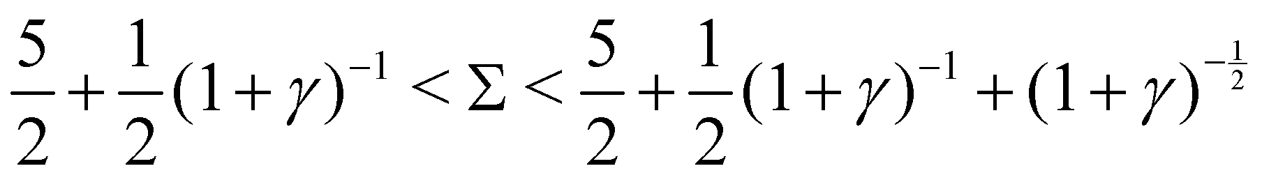 :
: :
:
 is the dissipation function derived in the Appendix. Near the equilibrium where θ1 ≈ θ2 ≪ 1, they can be approximated by
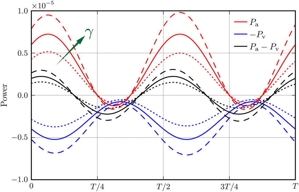
 represents the Lagrangian of the system
  where
where 
 corresponding to eqn (20) is defined as62
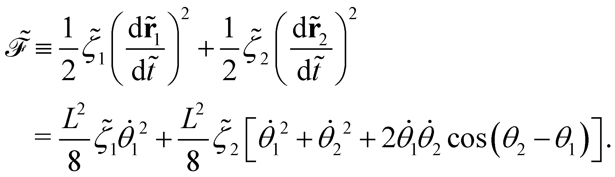
 offers two physical interpretations. Firstly, it represents the velocity-dependent potential, wherein the hydrodynamic force can be computed as
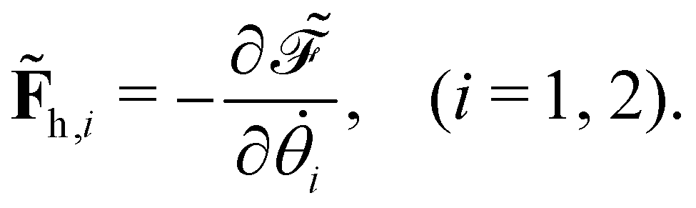
 with the potential energy Ṽ written as: