Excited state properties of an A–D–A non-fullerene electron acceptor: a LC-TD-DFTB study†
Received
19th December 2023
, Accepted 5th April 2024
First published on 5th April 2024
Abstract
Understanding charge transfer processes is essential to estimate the performance of organic photovoltaic technologies. Although experimental production is on the rise, predictability strongly relies on theoretical modeling, which is limited to the size of semiconductors. As a computationally favorable approach, we benchmarked the long-range corrected (LC) time-dependent (TD) formulation of the semi-empirical density functional-based tight-binding method (DFTB) for three polycyclic aromatic hydrocarbons (PAHs) and studied the DTP-IC-4Ph molecule, a PAH-based non-fullerene electron acceptor (NFA) with an A–D–A backbone structure. After a thorough investigation into the long-range parameter (ω) tuning for naphthalene, anthracene and pyrene, the excitation energies, oscillator strengths and Natural Transition Orbitals (NTOs) were compared with the standard ωB97X-D/6-31G(d,p) level of theory and the ADC2/6-31G(d,p) multiconfigurational method. We estimated mobility-related properties of the NFA and considered 1000 thermally accessible configurations to qualitatively reproduce the experimental absorption profile and investigate the energetic disorder. Finally, we conducted a fragment-based analysis using the one-electron transition density matrix (1TDM) to determine the character of the excited states and investigate the effect of side chains on exciton formation. Our results are sensitive to the level of theory and highly dependent on the long-range parameter but suggest that the presence of alkyl chains promotes a higher average charge delocalization and allows for additional hopping mechanisms, favoring the charge transfer dynamics.
1 Introduction
Among several applications of moderate-sized organic semiconductors, the so-called non-fullerene electron acceptors (NFAs)1,2 have been attracting attention for being strongly related to the recent growth in organic solar cell (OSC) performances.3 These molecules are typically formed as fused-ring structures with electron-donating and withdrawing moieties coupled to extensive side chains. Due to the high flexibility in molecular design, these acceptors have easily tunable bandgaps, energy levels and morphological properties,4,5 which overcome fullerene-based acceptor limitations and result in higher power conversion efficiencies (PCEs).6
Despite the remarkable progress in device performance, an appropriate understanding of the charge transfer processes, which integrate the energy conversion chain of events, remains elusive. In a simplified model, light absorption forms an electron–hole pair, also known as an exciton. Ideally, at the donor (D) and acceptor (A) molecule's interface, the HOMO and LUMO energy offset induces this quasi-particle to dissociate, which enables the charge carrier's diffusion toward the electrodes. In practice, several effects impact the exciton quenching, such as charge recombination,7 energetic disorder8 and crystallinity,9 resulting in different theoretical models. Regardless of the approach, quantum mechanics calculations are essential to describe the exciton dynamics but are also limited by the size of most systems, usually relying on density functional theory (DFT).10
Within the manifold of exchange–correlation (xc) functionals available in DFT, those that incorporate long-range correction (LC) have emerged as the popular choice for investigating charge-transfer processes in organic semiconductor molecules.9–17 The additional flexibility from the Coulomb interaction decomposition manages to satisfy Janak's theorem18 and the energy linearity theorem for fractional occupations,19 reducing the self-interaction error (SIE)20 and, for the first time in the DFT framework, resulting in consistently accurate orbital energies.21 Despite the achievement, dealing with these moderate-sized molecules limits the systems to a pair of NFAs or a few monomers of electron donor polymers, which motivates the usage of alternative methodologies.
In the present work, we explore a fast semi-empirical branch of DFT, the long-range corrected density functional based tight-binding method (LC-DFTB), along with its time-dependent counterpart. Similar to LC-DFT, the effectiveness of this approach is dependent on the precise tuning of the long-range parameter (ω) in the xc functional.22–25 When appropriately tuned, this methodology can significantly improve the accuracy of both orbital energies and the description of charged molecules.26 Despite the limitations in characterizing the first excited state of unsaturated molecules,27 LC-TD-DFTB has successfully reproduced long-range corrected time-dependent density functional theory (LC-TD-DFT) results28 and experimental data involving CT excitations29 of small organic molecules. In the context of OSCs, the semi-empirical method was employed to study the effect of different donor:acceptor (D:A) architectures on charge transfer30 and even made it computationally accessible to perform non-adiabatic dynamics for molecules of this size.31
Regarding the studied NFA, the so-called DTP-IC-4Ph (Fig. 1b) features an A–D–A backbone structure. The pyrene (C16H10) core has extensive π-conjugation, resulting in highly delocalized orbitals that increase the molar absorption coefficient and charge carriers mobility, both essential for organic semiconductors. This molecule was introduced by Wang et al.32 along with other polycyclic aromatic hydrocarbon (PAH)-based electron acceptors, and achieved the highest PCE of the family, 10.37% in a single-junction cell with PBDB-T polymer as the donor. Despite the lower efficiency when compared with state-of-the-art OSCs,33–37 DTP-IC-4Ph:PBDB-T is a low-cost additive-free heterojunction. The acceptor production cost is less than one-tenth of most NFAs38 and the absence of additives is important to enhance the device stability, increasing its lifetime.39 Therefore, it is a promising candidate from both experimental and theoretical perspectives.
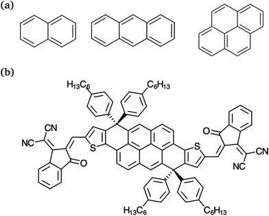 |
| | Fig. 1 Molecular structures of (a) PAHs naphthalene, anthracene and pyrene (from left to right) and (b) the non-fullerene electron acceptor DTP-IC-4Ph. | |
The sections are structured as follows: initially, a benchmark concerning the excited state properties of three PAHs, naphthalene, anthracene and pyrene (Fig. 1a), is performed for LC-TD-DFTB. Geometry and ω optimizations are compared to the standard DFT level of theory. At the same time, careful investigation is carried out to assess the dependence between tuned parameters, optimization procedures and exchange–correlation functionals. Excitation energies, oscillator strengths and natural transition orbitals (NTOs) at the LC-TD-DFTB level of theory are confronted with results from LC-TD-DFT and a reference wavefunction-based method. Once the comparison is established, we investigate the side chain's impact on light absorption of the NFA and average the LC-TD-DFTB absorption spectra over a set of thermally accessible nuclear configurations to reproduce the experimental profile qualitatively. A quantitative fragment-based analysis of the NFA excited states is also presented to provide further insights into the excitation character. Finally, the dielectric constant (ε), internal reorganization energies (λe/hin), exciton binding energies (Eb) and energetic disorder are estimated for the organic semiconductor using the semi-empirical approach.
2 Methods
This section introduces the theory directly related to this paper; further details can be found in the literature presented throughout the text. First, LC-TD-DFTB linear response matrix formulation is briefly discussed, focusing on the long-range correction. Then, the Clausius–Mossotti relation elucidates the electric constant evaluation. At the same time, Nelsen's four-point model determines the internal reorganization energies, and the fragment-based analysis concludes this section by presenting the excited-state descriptors computed in this work.
2.1 LC-TD-DFTB
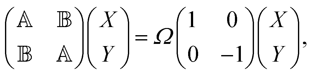
Among different approaches to characterize the electronic excited states spectra, linear response formalism is well-established in the TD-DFT community. As a DFT flavor, the LC-TD-DFTB method follows the same path of solving the generalized eigenvalue equation,40| | 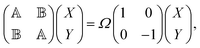 | (1) |
where X and Y vectors determine the transition density matrix and oscillator strengths related to the excitation energy Ω.  matrix elements are expressed in terms of the coupling matrix K,
| |  | (2) |
| |  | (3) |
A pair of indexes a, a′ and i, i′ concern the occupied and unoccupied orbitals, respectively, while σ and σ′ are the spin projections. The energy difference between a′ and i′ orbitals for the σ′ single-particle excitation is represented by  , and, in the density matrix formulation, the coupling matrix elements are given by
| | 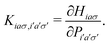 | (4) |
In LC-TD-DFT, the Hamiltonian element in eqn (4) is defined as the two-center double integral of the Coulomb operator (decomposed in short and long-range contributions) and exchange–correlation kernel over Kohn–Sham (KS) orbitals.40 On the other hand, LC-TD-DFTB formulation yields a modified operator that is integrated over localized KS-like orbitals as a consequence of the energy expansion up to second order around the density of free atoms and the addition of a confinement potential.29 However, in both approaches, the coupling matrix is determined in terms of xc kernels from the general energy expression,| | | Exc(ω) = ELR-HFx(ω) + ESR-HFx(ω) + ESR-DFTx(ω) + Ec. | (5) |
Several exchange and correlation functionals have been proposed, but for long-range correction, the standard error function decomposition41 and Yukawa exponential kernel partitioning42 are the common Ewald split of the Coulomb operator, both presented below, respectively,| | 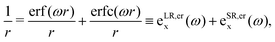 | (6) |
| | 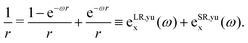 | (7) |
In general, both decompositions have similar behavior, but they can influence the adjustment of the long-range parameter, as discussed in the following sections.
2.2 Long-range parameter optimization
In most long-range corrected xc functionals, the default ω value ranges between 0.2 and 0.3a0−1 (Bohr−1), but common practice is to optimize the parameter by imposing Janak's theorem18 (also known as IP theorem). A direct consequence is that the vertical ionization potential (IP) becomes equal to the negative of HOMO energy, motivating the adjustment of ω in order to establish this identity, i.e., minimize the sum,| | | J1 = |εHOMO(N, ω) + IP(N, ω)|, | (8) |
where IP is given by the difference between the neutral and cation total energies at the ground state geometry. This relationship also stands for ionic systems, so Stein et al.43 proposed a similar criterion,| | | J2 = |εHOMO(N, ω) + IP(N, ω)| + |εLUMO(N, ω) + EA(N, ω)|, | (9) |
which relates IP(N + 1, ω), also known as electron affinity (EA), with the LUMO energy. Even though there is no formal equivalence between εLUMO(N, ω) and εHOMO(N + 1, ω), the results are essentially identical22,43 and we intended to verify it for LC-DFTB. The last criterion adopted has been used by Hirao et al.24 and is related to the Mulliken rule for charge-transfer.22 In this case, the difference between εHOMO and the energy of the unoccupied β-spin–orbital that pairs the singly occupied molecular orbital (SOMO) of the cation is minimized via,| | | J3 = |εHOMO(N, ω) − εβSOMO(N − 1, ω)|. | (10) |
2.3 Mobility-related properties
Among charge-transfer models, the semiclassical two-state Marcus equation44 has been the standard choice to determine the transfer rate of charge carriers between donors and acceptors.9,13,16 This kind of approach is well suited for strong couplings between CT and ground states,45 but refinements have been proposed to introduce vibrational effects46 and even include a third state in the model.47 Aside from the diabatic coupling between states, the reorganization energy (λ) related to the charge transfer between both states is a common element in each model. In this sense, we determined the internal contribution of the reorganization energy (λin) for both hole and electron via Nelsen's four-point method,48| | | λh/ein = (E±0 − E±) + (E0± − E0), | (11) |
with E0 and E+0(E−0) being the neutral and cation(anion) energy calculated at the ground state geometry, E+(E−) the cation(anion) energy at the cation(anion) geometry itself and E0+(E0−) the neutral state energy calculated at cation(anion) geometry. Exciton binding energy (Eb) was also estimated by the difference between fundamental and optical gaps,| | | Eb = Efundgap − Eoptgap, | (12) |
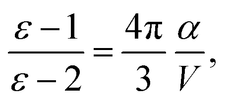
where Efundgap is the difference between IP and EA determined from total energy differences, and Eoptgap is the energy of the lowest excited state accessible via single photon absorption.49 Lastly, dielectric constants (ε) are part of continuum solvation models, which are frequently incorporated to simulate the presence of other D and A units, so they were estimated according to the Clausius–Mossotti relationship,50| |  | (13) |
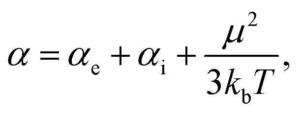
where α and V are the molecular polarizability and volume, respectively. The former can be decomposed in three parts,50 the electronic (αe), ionic (αi) and orientational polarizabilities,| |  | (14) |
which considers not only the charge density but crystallinity properties and the temperature (T) effect over the electric dipole moment (μ) ordering. Since the ionic contribution is only significant for periodic systems, we only considered the electronic and orientational parts. The static electronic polarizabilities were determined from finite field calculations51 for both DFT and DFTB levels of theory, as implemented in Gaussian16 and DFTB+, respectively. On the other hand, molecular volume is not strictly defined and was expressed in terms of electronic densities and van der Waals radii.
2.4 Excited states analysis
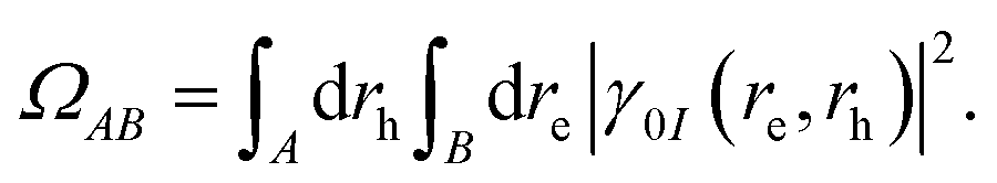
A fragment-based analysis of excited states using the one-electron transition density matrix (1TDM) formulation was employed to understand the exciton structure. From the 1TDM between the ground and the I-th excited state, given by,| |  | (15) |
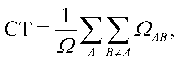
where re, rh, Ψ0 and ΨI are the electron and hole coordinates followed by ground and excited state wavefunctions, respectively, one can decompose the excitation into different spatial contributions. Out of the several descriptors available, for a pair of fragments A and B, the CT number is a crucial one that is determined according to,| |  | (16) |
By constraining the integration, it gives the probability of finding the hole on fragment A with the electron on fragment B, serving as a base for the definition of other excited-state descriptors, such as the CT character,| |  | (17) |
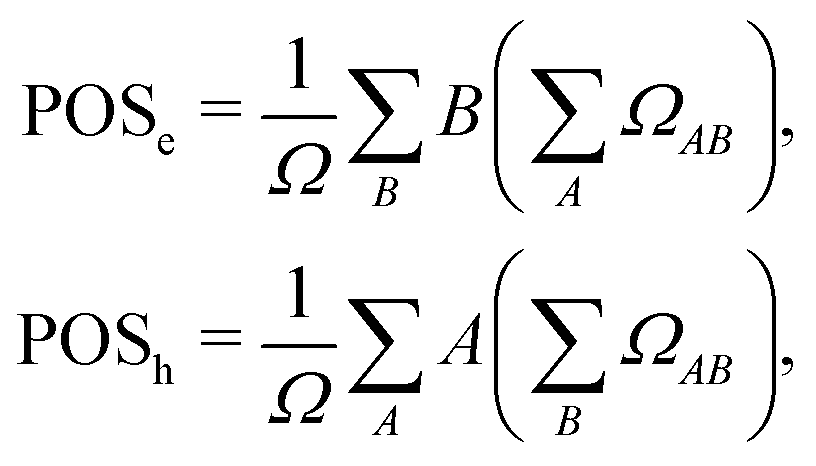
where  and the position descriptors for electrons (POSe), holes (POSh) and excitons (POS), which are given by
| |  | (18) |
| |  | (19) |
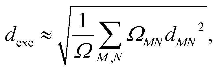
These expressions assume that fragments can be ordered, so A = 1, B = 2 and so on. The excitons can be characterized from the CT and POS descriptors by considering three fragments representing the A–D–A backbone of an NFA, A and C as acceptor and B as the donor moieties. Ideally, Frenkel excitons localized on the acceptor (LA) and donor (LD) will have (CT = 0.0, POS = 1.0/3.0) and (CT = 0.0, POS = 2.0), respectively, while for ideal CT states (CT = 1.0). An exciton size descriptor (dexc) is obtained due to the interpretation of 1TDM as the exciton wavefunction to quantify the delocalization. It can be approximately evaluated using atomic pairs52via,| | 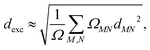 | (20) |
where ΩMN is the charge transfer number (16) computed with respect to two atoms M and N, and dMN is the distance between these atoms.
3 Computational details
3.1 Electronic structure calculations
Time-dependent and independent DFT calculations were performed with the Gaussian16 code.53 We employed two exchange–correlation functionals, ωB97XD and CAM-B3LYP along with 6-31G(d,p), so the methods will be referred to as ωB97XD/6-31G(d,p) and CAM-B3LYP/6-31G(d,p). The 6-31G(d,p) basis set is commonly used for moderate-sized molecules,9,14 and we found it to have minimal impact on the excited states of the PAHs, as exemplified by the absorption spectrum of naphthalene in the ESI.† LC-DFTB calculations were carried out with the DFTB+ software,54 employing the Baer, Neuhauser and Livshits (BNL) xc functional.55,56 In this approach, short-range exchange contributions were treated in the local density approximation (LDA), and long-range exact exchange interactions were accounted for through a descreened electron–electron interaction (LR part of eqn (7)). For the Slater–Koster (SK) files, a new parameterization of the OB2 set including sulfur atoms (n-OB2) was employed with a Slater–Kirkwood dispersion model. Both SK files and dispersion parameters were taken from previous work30 and are given in the ESI.† In addition to the two methods presented above, excited states and natural transition orbitals (NTOs) were also computed with the second-order Algebraic Diagrammatic Construction method and the 6-31G(d,p) basis set (ADC(2)/6-31G(d,p)) employing the adcc code57 interfaced with the PySCF package.58
Molecular volumes in the Clausius–Mossotti relationship (13) were estimated as the region with electronic density above 0.001a0−3 and using DFT-D3 van der Waals radii,59 for DFT and DFTB calculations, respectively. Further details are presented in the ESI.†
3.2 Excited states characterization
Fragment-based exciton analysis employed Löwdin populations and was performed via TheoDORE60 code, with the linear response data obtained from DFTB+54 and Gaussian16.53 Newton-X61 software was also employed to estimate absorption cross-sections using the nuclear ensemble approach.62 Nuclear configurations were generated from Wigner sampling at T = 300 K, while the oscillator strengths and excitation energies were obtained from the LC-TD-DFTB/n-OB2 method described above.
4 Results and discussion
4.1 Long-range parameter
The n-OB2 parameters are available for a few values of the range-separation parameter,30 specifically ω = 0.1, 0.2, 0.3, 0.4 and 0.5a0−1, which allow for partial optimization of the Ji criteria described in Section 2.2. In contrast, the DFT methods can vary the ω values without restriction. While recent LC-TD-DFTB studies of donor:acceptor interface models30,63 have discussed the optimization of the ω parameter, the procedures have not been thoroughly tested in the DFTB framework compared to DFT.21,25,43,64–66 We therefore consider the PAH molecules naphthalene, anthracene and pyrene along with the organic semiconductor.
4.1.1 PAHs.
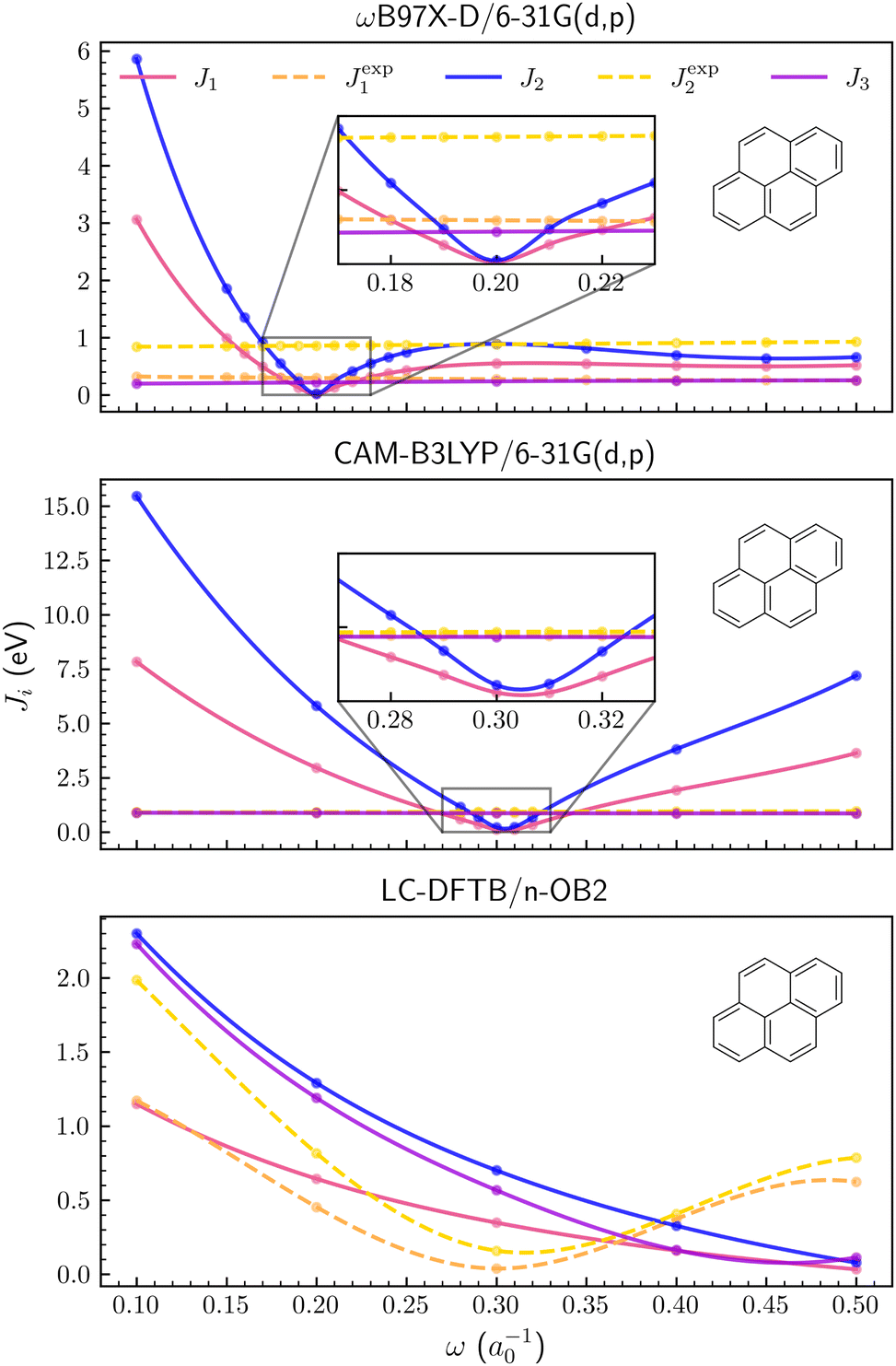
The Ji functions are shown for pyrene in Fig. 2, while the corresponding plots for naphthalene and anthracene are available in the ESI.† Optimal ω values for the three PAH molecules are also summarized in Table 1. Although the results depend on the xc functional, the tuning based on the J1 and J2 criteria provided similar optimal values for both the ωB97X-D/6-31G(d,p) and CAM-B3LYP/6-31G(d,p) methods (see Table 1). In contrast, J3 is a much smoother function of the ω parameter, compared to J1,2 (Fig. 2), and the corresponding optimal values are somewhat discrepant, especially for the CAM-B3LYP functional. The agreement between tuned parameters obtained from J1 and J2 could not be easily anticipated since the compact basis set 6-31G(d,p) might not be adequate to estimate the energies of the anion forms, which are necessary to compute the EAs. Apart from the differences arising from the xc functionals, which could be expected, the tuning procedures based on DFT and the J1,2 criteria seem consistent, providing optimal values in agreement, ω ≈ 0.20a0−1 and ω ≈ 0.30a0−1 respectively for the ωB97X-D and CAM-B3LYP functionals.
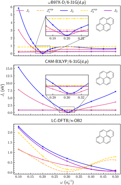 |
| | Fig. 2 Optimization criteria J1, J2, J3, Jexp1 and Jexp2 as a function of long-range parameter for the pyrene molecule. From upper to lower panel, ωB97X-D/6-31G(d,p), CAM-B3LYP/6-31G(d,p) and LC-DFTB/n-OB2 levels of theory were employed, respectively. | |
Table 1 Optimized values of long-range parameter (a0−1 units) obtained via J1, J2 and J3 criteria for each PAH. Jexpi columns adopted experimental values of IP and EA. The atomic basis 6-31G(d,p) was employed for both DFT calculations
| System |
Method |
J
1
|
J
2
|
J
3
|
J
exp1
|
J
exp2
|
| Naphthalene |
ωB97X-D |
0.21 |
0.18 |
0.25 |
0.50 |
0.10 |
| CAM-B3LYP |
0.28 |
0.28 |
0.50 |
0.50 |
0.26 |
| LC-DFTB |
0.50 |
0.50 |
0.50 |
0.30 |
0.30 |
|
|
| Anthracene |
ωB97X-D |
0.20 |
0.20 |
0.10 |
0.50 |
0.10 |
| CAM-B3LYP |
0.30 |
0.30 |
0.50 |
0.50 |
0.10 |
| LC-DFTB |
0.50 |
0.50 |
0.50 |
0.30 |
0.30 |
|
|
| Pyrene |
ωB97X-D |
0.20 |
0.20 |
0.10 |
0.50 |
0.10 |
| CAM-B3LYP |
0.31 |
0.30 |
0.50 |
0.50 |
0.10 |
| LC-DFTB |
0.50 |
0.50 |
0.50 |
0.30 |
0.30 |
Following Hirao et al.,25 we also calculated the J1 and J2 functions using the experimental IP and EA values (available in Table S2 and the ESI†), indicated as Jexp1,2 in Fig. 2 and Table 1. Both functions are roughly constant for the ωB97X-D/6-31G(d,p) and CAM-B3LYP/6-31G(d,p) calculations. Restricting the discussion to J1 for simplicity, this behavior can be easily understood. The calculated IPs generally increase as a function of the long-range parameter, while the HOMO energies, εHOMO, are smoother functions of ω (roughly constant, see the ESI†). The J1 functions therefore show minima as the IP curves cross the εHOMO ones. In contrast, the |εHOMO − IPexp| absolute differences vary slowly, where IPexp is the experimental IP.
Despite the restricted set of ω values described above, the same tuning procedures were carried out with the LC-DFTB/n-OB2 method. The behavior of the J1,2,3 functions remarkably differ from those computed with DFT-based methods (see Fig. 2). None of those functions seem to have a minimum within the 0.1a0−1 ≤ ω ≤ 0.5a0−1 range. A decreasing trend is observed for the calculated points such that the smallest J1,2,3 values are found for ω = 0.5a0−1 (not necessarily minima), where the curves also approach each other. In contrast to the DFT results, the Jexp1,2 curves, obtained from the experimental IP and EA as above, show minima around ω = 0.3a0−1 for the three PAH molecules (see Fig. 2 and the ESI†). Restricting the discussion to J1 once more, both the IP and εHOMO, computed with LC-DFTB/n-OB2, are increasing functions of the ω parameter, such that J1 slowly decreases while Jexp1 shows a minimum as εHOMO goes through the experimental IP value.
For the PAH molecules, the IPs computed with DFT and DFTB methods tend to increase as functions of ω, although the DFT estimates become almost constant for sufficiently large ω (see the ESI†). The most striking difference between DFTB and DFT results is the HOMO energies' dependence on the LC parameter, which is stronger in the semi-empirical approach. While the orbital energies are significantly improved by the LC screening of self-interaction errors,21 it is not a simple matter to understand the differences between the εHOMO estimates computed with DFT and DFTB, given the several different approximations underlying the tight binding method (see Section 2.1). Nonetheless, one could consider a couple of aspects more directly related to the LC, namely HF exchange in the short-range region and the screening functions. The LC-DFTB method is built on the BNL functional, which does not include short-range HF exchange,26 and the lack of that term could affect the results. For instance, the ωB97X functional (and hence ωB97X-D), which does include the HF exchange term, generally performs better than the ωB97 counterpart, which does not include that exchange term.67 Finally, the ωB97X-D functional and LC-DFTB respectively employ error function and Yukawa kernels, according to eqn (6) and (7) (a modified error function decomposition is used in CAM-B3LYP68). Since the erfc function decays faster than the Yukawa one for a given LC parameter, the spatial decomposition into short- and long-range regions of similar sizes requires larger exponents in the Yukawa function (see also the ESI†).
Regardless of the main sources of error, one can assess the quality of the results obtained with the tuned ω values. The calculated vertical IP and εHOMO for pyrene are shown in Table 2 along with the experimental IP69 and a reference value of the HOMO energy computed with the MP3/6-31G+(d,p) method70 (see the ESI† for the other PAH molecules). For the ωB97X-D/6-31G(d,p) method, the IP and εHOMO calculated with the tuned parameter (ω ≈ 0.2a0−1) disagree with the reference values by 0.28 eV and 0.17 eV, respectively. For LC-DFTB/n-OB2 (ω ≈ 0.5a0−1), the disagreement is much more significant, around 0.66 eV and 1.09 eV respectively for the IP and HOMO energy. In case Jexp1 is used to tune the LC parameter (ω ≈ 0.3a0−1), the HOMO energy is improved by 0.27 eV (while the IP error is of course removed). For LC-DFTB/n-OB2, the LC parameter tuned with the J1 criterion overly binds the electron, thus suggesting some imbalance in the exchange energy.
Table 2 Ionization potential (IP) and HOMO (εHOMO) energies for pyrene. The 6-31G(d,p) basis set was employed along with the ωB97X-D functional
| Method |
ω (a0−1) |
IP (eV) |
ε
HOMO (eV) |
| ωB97X-D |
0.1 |
4.045 |
−7.105 |
| 0.2 |
7.145 |
−7.131 |
| 0.3 |
7.701 |
−7.153 |
| 0.4 |
7.678 |
−7.166 |
| 0.5 |
7.692 |
−7.174 |
| LC-DFTB |
0.1 |
7.404 |
−6.254 |
| 0.2 |
7.616 |
−6.972 |
| 0.3 |
7.812 |
−7.464 |
| 0.4 |
7.958 |
−7.798 |
| 0.5 |
8.082 |
−8.048 |
| Ref. |
— |
7.42669 |
−6.95770 |
4.1.2 DTP-IC-4Ph.
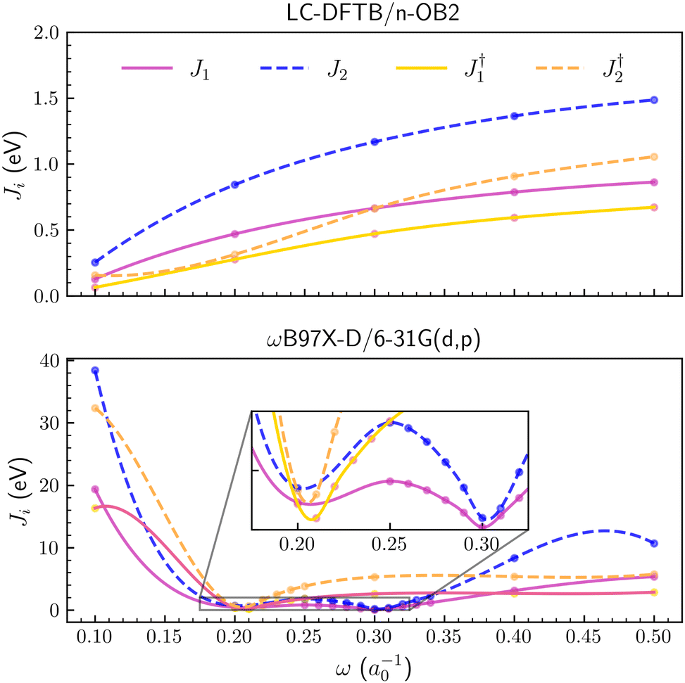
The LC parameter was also tuned for the DTP-IC-4Ph acceptor with the J1,2 criteria. As shown in Fig. 3, we considered the molecule with and without the alkyl side chains (C6H13 groups, see Fig. 1b). For LC-DFTB/n-OB2, the J1,2 functions approach each other as the LC parameter decreases for both DTP-IC-4Ph forms, so the smallest values are obtained for ω = 0.1a0−1. The optimal ω values generally decrease with the system size since the semilocal approximations to the exchange–correlation functional tend to be more reliable as the orbitals delocalize.65 Therefore, the lack of short-range HF exchange, one of the sources of error of the LC-DFTB/n-OB2 calculations, would not be as stringent for DTP-IC-4Ph compared to the PAHs. The standard tuning procedures based on the J1,2 functions seem more reliable for the DTP-IC-4Ph acceptor (with and without the alkyl chains) than for the smaller systems.
 |
| | Fig. 3 Optimization criteria J1 and J2 as a function of long-range parameter for the DTP-IC-4Ph molecule. In the upper and lower panels ωB97X-D/6-31G(d,p) and LC-DFTB/n-OB2 levels of theory were employed, respectively. The symbol † indicates the removal of alkyl groups. | |
For the ωB97X-D/6-31G(d,p) method, geometry optimization significantly affected the tuning. In case the J1,2 functions were computed for a fixed geometry, the tuned ω values for the DTP-IC-4Ph forms, differing with respect to the alkyl chains, were below 0.1a0−1, consistent with previous results for other NFA molecules9,13,71,72 (see the ESI† for details). However, when the molecular geometries were reoptimized for every ω value, the J1,2 functions presented a double-minimum structure, as shown in Fig. 3, where the slightly deeper one was found at ω ≈ 0.3a0−1. The PAH molecules and the DTP-IC-4Ph acceptor do not merely differ by size or number of monomers but by chemical elements (nitrogen and sulfur) and several chemical groups. While the results for a fixed geometry show the usual trend between the tuned LC parameter and the system size, the geometry optimization increased the ω values tuned for ωB97X-D/6-31G(d,p).
4.2 Excited states
Before addressing the NFA, we compare the excitation spectra and NTOs for the PAH molecules with the LC-TD-DFTB/n-OB2 and the time-dependent ωB97X-D/6-31G(d,p) methods. While our main interest is comparing the TD-DFT and TD-DFTB calculations, we also obtained ADC2/6-31G(d,p) results for those smaller molecules. The wave function-based polarization propagator method has successfully described electronic excitations and the location of charge-transfer (CT) states in organic systems,73,74 being employed as a reference to benchmark TDDFT calculations.75
4.2.1 PAHs.
Vertical excitation spectra of the PAH molecules were computed with the LC parameters tuned with the J1 criterion (see Table 1). For both the LC-TD-DFTB/n-OB2 and TD-ωB97X-D/6-31G(d,p) methods, the ground state geometries were optimized with the respective time-independent methods using the tuned ω values. The bond lengths and angles obtained were compatible, presenting a small root mean square deviation of 0.0115 Å between the DFT and DFTB geometries. Thus, the ωB97X-D/6-31G(d,p) ground state geometry was employed in the ADC2/6-31G(d,p) calculations.
Fig. 4 shows the excitation energies and oscillator strengths of the first excited state (S1) and the brightest among the lowest ten excited states (SB) of pyrene. We also show the hole and particle orbitals for each excitation, described as natural transition orbitals (NTOs) for the TD-ωB97X-D/6-31G(d,p) and ADC2/6-31G(d,p) calculations, while canonical molecular orbitals for the LC-TD-DFTB/n-OB2 counterpart. In the latter case, the S1 and SB excited states have dominant contributions from single electron–hole orbital pairs, making the comparison with the NTOs meaningful (see Section S2.1 of the ESI†). For the first excited state, there is reasonable agreement between the TD-DFT and TD-DFTB energies (4.07 eV and 4.13 eV, respectively), which are slightly higher than the ADC energy (3.90 eV). These results are consistent when compared to the data-driven benchmark performed by Bertoni and Sanchez.27 Despite employing a different xc functional with an ω-optimization step, we obtained S1 energy differences between the DFT-based methods smaller than 0.5 eV, as expected for most π-conjugated molecules. For the brightest state, the agreement between the TD-DFT and ADC2 energies is remarkable (5.85 eV and 5.89 eV, respectively), while a higher value was obtained with TD-DFTB (6.00 eV). For both states, the excitation energies computed with the three methods agree within 0.2 eV, but the discrepancies for the oscillator strengths can be viewed as more significant. While the oscillator strengths predicted by the different methods for the SB state vary from f = 0.88 (TD-DFTB) to f = 1.15 (ADC2), there is a qualitative difference for the lowest excitation. The S1 state is fairly bright according to the TD-DFTB method (f = 0.353), but dark (f ∼ 10−4) according to the other methods. It is clear from Fig. 4 that the hole orbital has a different character in the TD-DFTB calculation, and further inspection of the excitation spectra indicates that the second excited state obtained from the TD-DFTB calculation (not shown) has the same character as the S1 dark states predicted by the TD-DFT and ADC2 methods. This discrepancy indicates that the calculated excitation spectra can be highly sensitive to geometry changes and the tuning of the LC parameter, even for small molecules. As discussed below, the excitation spectra computed with the nuclear ensemble method are more consistent than vertical spectra.
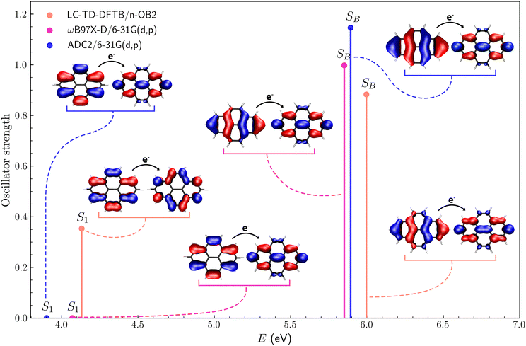 |
| | Fig. 4 First (S1) and brightest (SB) excited states of pyrene along with the corresponding hole and electron orbitals obtained via LC-TD-DFTB/n-OB2, ωB97X-D/6-31G(d,p) and ADC2/6-31G(d,p) calculations. | |
4.2.2 DTP-IC-4Ph.
As in most organic photovoltaics (OPV) materials, the PAH-based acceptor has side chains incorporated to increase solubility. The alkyl groups generally reduce the planarity of the π-conjugated cores and affect the aggregation of heterojunctions, although without actively participating in radiation absorption. In the following, we calculate the DTP-IC-4Ph spectrum with and without the side chains to assess to which extent the alkyl groups could indirectly affect the excited states (e.g., through orbital delocalization or geometry changes). We also compare the TD-DFT and TD-DFTB models along the lines of the previous sections.
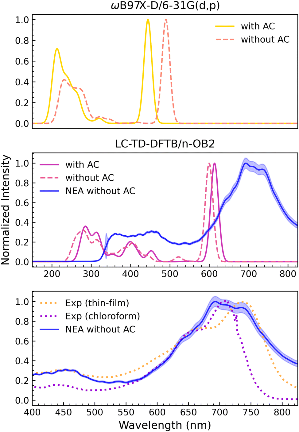
The vertical spectra computed with the TD-ωB97X-D/6-31G(d,p) method for both DTP-IC-4Ph forms are shown in the upper panel of Fig. 5. As discussed above (see Fig. 3), the J1,2 functions obtained for DTP-IC-4Ph have double-minima structures. The acceptor molecule without the alkyl chains (ACs) shows a slightly deeper minimum around ω = 0.2a0−1, while the minimum around ω = 0.3a0−1 becomes slightly deeper as the ACs are incorporated. The absorption spectra calculated with the corresponding ω values are somewhat discrepant since the peaks are shifted between molecules with and without ACs. For the strong absorption peak around 500 nm, the deviation is approximately 60 nm (≈0.34 eV). We also recomputed the spectrum for the molecule without the ACs using ω = 0.3a0−1, which essentially removed the disagreement (see the ESI†). While it is clear that the shifts mainly arise from the different ω values (not the inclusion of the ACs), one is faced with difficulty in the optimization procedure. The better choice of the range separation parameter, ω = 0.2a0−1 or ω = 0.3a0−1, is not evident a priori. In practice, ω = 0.3a0−1 provided better results since the strong absorption around 500 nm seems more compatible with the experimental data (see below).
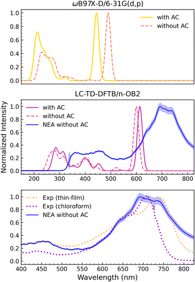 |
| | Fig. 5 Normalized absorption spectra of DTP-IC-4Ph. Top panel: ωB97X-D/6-31G(d,p) vertical spectra for the molecule (yellow) and without (orange) alkyl chains (ACs). Central panel: LC-TD-DFTB/n-OB2 vertical spectra with (magenta) and without (pink) ACs. The NEA LC-TD-DFTB/n-OB2 calculation is also shown for the molecule without ACs (blue). Lower panel: Comparison between the NEA LC-TD-DFTB/n-OB2 calculation in vacuum (blue) with the experimental data32 measured from a thin-film (orange) and from a chloroform solution (purple). | |
The central panel of Fig. 5 shows the spectra computed with the LC-TD-DFTB/n-OB2 method. In this case, the same optimal value of the range-separation parameter (ω = 0.1a0−1) was obtained for both DTP-IC-4Ph forms. The vertical absorption spectra are mildly affected by the ACs despite the more prominent structures between 350 nm and 550 nm. The vertical-approximation results obtained for the DTP-IC-4Ph acceptor and even for the smaller PAH molecules are somewhat sensitive to small changes in geometry, as discussed above. Exploring the computational efficiency of the LC-TD-DFTB/n-OB2 method, we recalculated the absorption spectrum of DTP-IC-4Ph without the ACs employing the nuclear ensemble approach (NEA). The spectrum was averaged over the Franck–Condon region with 1000 configurations (geometries) weighted according to the room-temperature Wigner distribution. The result is also shown in the central panel of Fig. 5 (blue line), where the most intense peak is broadened and shifted by ≈90 nm (≈0.25 eV). The downshift in energy concerning the vertical-excitation peaks essentially arises from vibrational frequency changes between the ground and the excited electronic states,76 while the broadening is due to the convolution of the vertical excitations. The lower-intensity peaks, around 250 nm to 550 nm, become convoluted into a broad and flat structure in the NEA calculation. Furthermore, the NEA curve profile oscillations indicate that 1000 configurations were not enough to fully converge the absorption cross section.77
In the lower panel of Fig. 5, the gas-phase NEA absorption spectrum is compared to the experimental data observed in thin films and in chloroform solvent.32 The improvement in shape brought about by the NEA average is remarkable. Nevertheless, the intensity of the high-energy band (around 450 nm) is overestimated with respect to the intensity of the low-energy one (around 700 nm), and the calculation also overestimates the absorption at higher wavelengths (above 750 nm). Unfortunately, continuum solvent models were unavailable for time-dependent calculations in the DFTB+ package. Despite the difficulty of pointing out the exact position of the most robust band in the NEA calculation, we estimate the peak to be overestimated in energy by 50 meV to 100 meV with respect to the experimental result obtained in chloroform. Since the solvatochromic effect should be relatively weak in view of the small dielectric constant (ε = 4.8 for chloroform), we would consider the position of the absorption maximum to be in good agreement with the data. As discussed in Section 4.1, the tuning procedure based on the IP theorem seemed more consistent for the DTP-IC-4Ph acceptor than for the smaller PAH molecules despite the limited set of ω values currently available for the LC-TD-DFTB/n-OB2 method. We also discussed the sensitivity of the energy and characters of the excited states to geometry changes. Despite those difficulties, the absorption spectrum calculated with ω = 0.1a0−1 within the NEA framework provided fairly accurate results at reasonable computational cost. The efficiency of TD-DFTB is, of course, important given the several configurations required by NEA to average out the geometry-related discrepancies in the vertical spectra and sufficiently account for the vibrational shift and broadening.
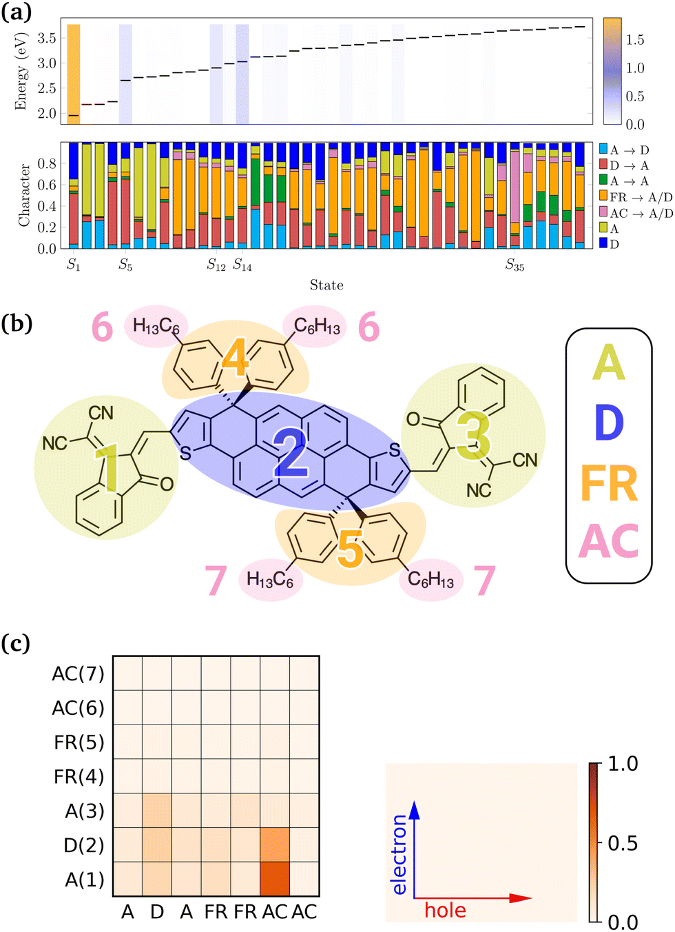
In order to investigate the character of excitations, the excited states that make up the LC-TD-DFTB/n-OB2 vertical spectrum were further analysed with the fragment-based decomposition. The DTP-IC-4Ph molecule was decomposed into the seven fragments shown in Fig. 6b, which were further classified as electron acceptor (A), electron donor (D), fused ring (FR) and alkyl chains (AC) moieties. From this decomposition, we can compute several excited state descriptors and identify the dominant contributions for each excitation. For example, the top panel in Fig. 6a shows the excitation energies and oscillator strengths (color bars) of the first 40 excited states of DTP-IC-4Ph (with alkyl chains), computed via the LC-TD-DFTB/n-OB2 method. On the bottom panel, the excitation character is decomposed into the dominant contributions, indicating in which fragments the holes/electrons are localized. For instance, the first two bright states S1 and S5 are mainly a combination of two types of excitation, from donor to acceptor moieties (red) and from localized excitation on the donor (blue). On the other hand, the following two bright states (S12 and S14) are defined by a mixture of different contributions.
 |
| | Fig. 6 Fragment-based analysis of DTP-IC-4Ph at the LC-TD-DFTB/n-OB2 level of theory. (a) Excitation energies and oscillator strengths (color bars) of the first 40 excited states are presented (top) along with the excited states character (bottom). (b) DTP-IC-4Ph divided into 7 fragments. (c) Electron–hole correlation plot of S35. Numbers in parentheses correspond to the fragments presented in (b). | |
We performed the fragment-based analysis considering the molecule with and without ACs, using the DFT/DFTB methods and for the distinct ground-state geometries. Although the slight differences between optimized configurations yield similar outcomes (see the ESI†), changes in size and method impact the overall results. For instance, increasing ω tends to localize the states as it decreases the short-range contribution of the exchange–correlation energy. Concerning the molecular composition, the S35 illustrates the sensitivity towards the presence of side chains. One should expect that C6H13 chains indirectly influence the FR → A/D contributions (orange bars in Fig. 6a) by changing the spatial orientation of the fused rings. However, for S35, the alkyl chains actively participate in the excitation, as indicated by the dominant bar in the bottom panel of Fig. 6a. As depicted by the electron–hole correlation plot in Fig. 6c, this excitation is mainly defined by transitions from the alkyl chains towards the A and D units, which are neglected when removing the side chains. Although AC → A/D transitions are not observed at the LC-TD-DFT level in this energy range (see the ESI†), the interchange between the character of excited states computed with each method has been previously reported for the smaller PAHs (see Fig. 4).
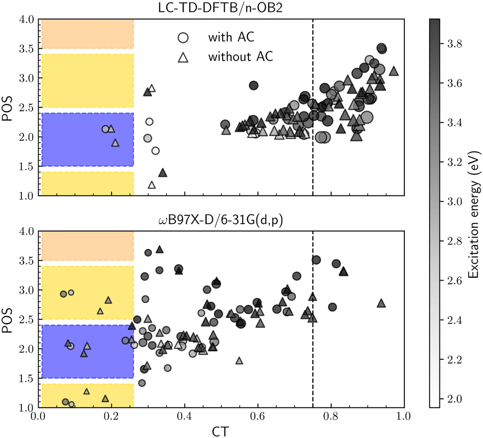
To investigate the excited state descriptors, Fig. 7 shows the average exciton position (POS) as a function of the charge-transfer number (CT) for both systems at each level of theory. The color bar plot also provides the excitation energies while the markers' size is proportional to the exciton size descriptor (dexc). Following our previous convention,30 the dashed line establishes the lower bound for charge-transfer states (CT > 0.75). At the same time, the colored regions indicate the localized states (CT < 0.25), with the colors corresponding to the different moieties presented in Fig. 6b, i.e., yellow for A, blue for D and so on.
 |
| | Fig. 7 Exciton average position (POS) and charge-transfer number (CT) descriptors of the first 50 excited states at the (a) LC-TD-DFTB/n-OB2 and (b) ωB97X-D/6-31G(d,p) levels of theory. The marker's size is proportional to the exciton size descriptor (dexc), and the color bar plot maps the excitation energy. Colored regions correspond to localized states in each fragment. | |
For both methods, the molecule with and without ACs has a similar behavior. The average exciton position is always located along the A–D–A backbone structure (POS < 4), and the higher energy states are more delocalized. Additionally, the number of localized states remains constant, indicating smaller exciton sizes than those with higher CT numbers. On the other hand, the level of theory has a direct impact on the overall charge delocalization. As an example, for the molecule with ACs, LC-TD-DFTB/n-OB2 yields average values of 〈CT〉 = 0.76 and 〈![[d with combining tilde]](https://www.rsc.org/images/entities/i_char_0064_0303.gif) exc〉 = 9.54 Å, in contrast to 〈CT〉 = 0.41 and 〈exc〉 = 5.68 Å with ωB97X-D/6-31G(d,p). Given the correlation between the descriptors and the choice of long-range parameter, these results reinforce the need for an ω-optimization protocol to study excited states.
exc〉 = 9.54 Å, in contrast to 〈CT〉 = 0.41 and 〈exc〉 = 5.68 Å with ωB97X-D/6-31G(d,p). Given the correlation between the descriptors and the choice of long-range parameter, these results reinforce the need for an ω-optimization protocol to study excited states.
4.3 Mobility-related properties
To complete the study, we determined relevant properties for charge transfer and investigated how IP and EA vary over the configurations. According to Table 3, internal intramolecular reorganization energies (λe/hin) exhibit an increasing trend in the presence of alkyl chains, consistent with a higher energy cost for accommodating the charge carriers in larger systems. Moreover, the exciton binding energy (Eb) is found to have a negative correlation with CT and exc, as weaker-bounded excitons are more susceptible to dissociation. For instance, at the DFTB level, the presence of side chains results in higher CT and exc values for the first accessible excited state (S1), leading to a smaller electron–hole Coulomb interaction and, subsequently, a reduction in Eb. The equivalent is observed for DFT calculations. However, in this case, the side chains reduce around 7% and 10% of CT and exc descriptors of S1 (see the ESI†), increasing the exciton binding energy. Since the character of S1 remains essentially the same, the difference in Eb is directly related to the change of ω. Adding side chains increases the optimized long-range parameter from 0.2a0−1 to 0.3a0−1, reducing the overall charge delocalization of excited states, as discussed in Section S2.2 of the ESI.†
Table 3 Dielectric constant (ε) at the ground state geometry, electron/hole internal reorganization energy (λe/h) and exciton binding energy (Eb) values for DTP-IC-4Ph
| System |
Method |
ε
|
λ
ein (eV) |
λ
hin (eV) |
E
b (eV) |
| DTP-IC-4Ph |
ωB97X-D |
3.908 |
1.288 |
1.268 |
2.808 |
| LC-TD-DFTB |
15.850 |
0.303 |
0.199 |
0.952 |
| DTP-IC-4Ph† |
ωB97X-D |
5.355 |
0.482 |
0.331 |
1.977 |
| LC-TD-DFTB |
5.745 |
0.264 |
0.181 |
1.367 |
For the dielectric constants (ε), opposite behaviors are observed for each method, which is strongly related to the orientation of side chains. In the semi-empirical approach, alkyl groups significantly increase the electronic polarizability (α) compared to the molecular volume expansion, and from eqn (13), it results in higher ε. On the other hand, although both quantities increase upon adding side chains, in DFT calculations, the increase in volume is more significant than that in polarizability. As a result, the dielectric constant of the complete molecule is reduced. As alkyl chains are quite flexible, one should expect that several orientations are observed experimentally, such that the average dipole moment is most likely to reproduce the DTP-IC-4Ph† value. Therefore, the ε without ACs is a better estimate to match experimental values.
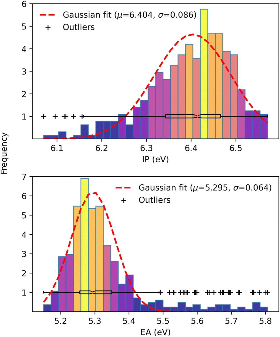
Finally, driven by the relationship between open-circuit voltage and static energetic disorder,71 we examined the IP and EA distributions over the ensemble of configurations from Wigner sampling. While the dynamic disorder is determined from temperature, the total disorder is estimated by the standard deviation of a Gaussian fit on IP and EA values obtained from configurations generated via MD simulations of D:A heterojunctions. In particular, we followed Brédas et al.71 and respectively approximated the IP and EA values from the HOMO and LUMO energies as a consequence of the close values due to the long-range parameter optimization procedure. Then, we fitted a normal distribution over the IP and EA values of 385 out of the 1000 configurations that converged during the self-consistent charge (SCC) scheme in the LC-DFTB method. The results are presented in Fig. 8.
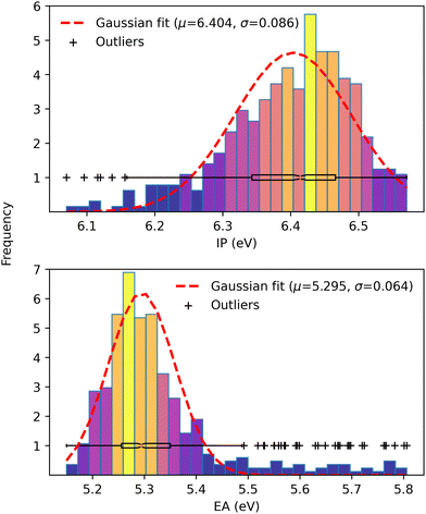 |
| | Fig. 8 Gaussian fit of IP (upper panel) and EA (lower panel) distributions over 385 configurations. The color code maps from low (blue) to high (yellow) frequencies. | |
Despite the bell shape, both distributions are irregular and asymmetric, most likely due to the small number of configurations. We used a boxplot to determine the outliers to estimate a standard deviation and fitted a normal distribution on the remaining data. Even though there is no formal correspondence between Wigner sampling and the classical configurations, the standard deviation of 0.064 eV is consistent with the total energetic disorder determined from 3000 MD configurations of high-efficiency small molecule NFAs,71 given by 0.054 and 0.052 eV for FNIC1 and FNIC2, respectively.
5 Conclusion
In this work, we benchmarked the LC-TD-DFTB method against the standard LC-TD-DFT level of theory for PAHs and a PAH-based NFA, focusing on evaluating the impact of long-range correction and the presence of side chains. An appropriate long-range parameter optimization procedure is required once it significantly influences the electronic structure, shifting absorption spectra and especially the character of the excited state. In particular, using experimental data as a reference for the tuning procedure proved to be beneficial only for the LC-DFTB method, failing to yield an optimal ω value at the LC-DFT level of theory.
When comparing both methods, the divergence is more pronounced in the character of excited states, switching the exciton distribution over the excitations. For anionic systems, a substantial underestimation of electron affinities is reported. The lack of exact short-range exchange interaction in the semi-empirical method is likely to play a significant role, as it results in higher ω optimized values, changing the overall electronic structure. From the PAH results, one can expect that, in the LC-TD-DFTB/n-OB2 approach, the brightest state character will be characterized appropriately. In contrast, the character of other excited states may be interchanged, triggering the photodynamics from the same starting point but leading to different pathways. Concerning the organic semiconductor study, side chains had a minor impact on the absorption spectrum profile. However, they significantly changed the excited state character, increasing the average exciton delocalization for DFTB-based calculations. Mobility-related properties are also strongly system and method-dependent. Ultimately, the tight-binding framework established a fast and flexible quantum description of computationally demanding systems, enabling the qualitative description of the organic semiconductor experimental absorption profile.
Author contributions
R. B. R. contributed to conceptualization, data curation, formal analysis, investigation, methodology, software, validation, visualization and overall writing. M. T. do N. V. contributed to conceptualization, formal analysis, funding acquisition, resources, supervision and overall writing.
Conflicts of interest
There are no conflicts to declare.
Acknowledgements
R. B. R. acknowledges financial support from CNPq (Grant no. 135967/2019-8), CAPES (Grant no. 8888.7644651/2021-00) and FAPESP (Grant no. 2022/04379-3). M. T. do N. V. also acknowledges financial support from CNPq (Grant no. 306285/2022-3) and FAPESP (Grant no. 2020/16155-7). The calculations were partly performed with HPC resources from STI, University of São Paulo, and Centro Nacional de Computação de Alto Desempenho (CENAPAD-SP). The authors also acknowledge Prof. Stephan Irle and Dr Van Quan Vuong for the Slater-Koster files and Dr Ljiliana Stojanović for supporting the fragment-based analysis.
Notes and references
- L. Zhan, S. Li, T.-K. Lau, Y. Cui, X. Lu, M. Shi, C.-Z. Li, H. Li, J. Hou and H. Chen, Energy Environ. Sci., 2020, 13, 635–645 RSC.
- A. Wadsworth, M. Moser, A. Marks, M. S. Little, N. Gasparini, C. J. Brabec, D. Baran and I. McCulloch, Chem. Soc. Rev., 2019, 48, 1596–1625 RSC.
- N. (National Renewable Energy Laboratory), Best Research-Cell Efficiencies, 2021, https://www.nrel.gov/pv/cell-efficiency.html.
- P. Cheng, G. Li, X. Zhan and Y. Yang, Nat. Photonics, 2018, 12, 131–142 CrossRef CAS.
- C. Yan, S. Barlow, Z. Wang, H. Yan, A. K. Jen, S. R. Marder and X. Zhan, Nat. Rev. Mater., 2018, 3, 1–19 CrossRef.
- G. Zhang, J. Zhao, P. C. Chow, K. Jiang, J. Zhang, Z. Zhu, J. Zhang, F. Huang and H. Yan, Chem. Rev., 2018, 118, 3447–3507 CrossRef CAS PubMed.
- C. W. Dan He, F. Zhao and Y. Lin, Adv. Funct. Mater., 2022, 32, 2111855 CrossRef.
- J. Yan, E. Rezasoltani, M. Azzouzi, F. Eisner and J. Nelson, Nat. Commun., 2021, 12, 1–12 CrossRef PubMed.
- G. Kupgan, X. K. Chen and J. L. Brédas, Mater. Today Adv., 2021, 11, 100154 CrossRef CAS.
- V. Bhat, C. P. Callaway and C. Risko, Chem. Rev., 2023, 123(12), 7498–7547 CrossRef CAS PubMed.
- G. Zhang, X. K. Chen, J. Xiao, P. C. Chow, M. Ren, G. Kupgan, X. Jiao, C. C. Chan, X. Du, R. Xia, Z. Chen, J. Yuan, Y. Zhang, S. Zhang, Y. Liu, Y. Zou, H. Yan, K. S. Wong, V. Coropceanu, N. Li, C. J. Brabec, J. L. Bredas, H. L. Yip and Y. Cao, Nat. Commun., 2020, 11, 1–10 CrossRef PubMed.
- T. Wang and J. L. Brédas, Matter, 2020, 2, 119–135 CrossRef.
- A. F. Marmolejo-Valencia, Z. Mata-Pinzón and C. Amador-Bedolla, Phys. Chem. Chem. Phys., 2021, 23, 16806–16815 RSC.
- L. Benatto, K. R. D. A. Sousa and M. Koehler, J. Phys. Chem. C, 2020, 124, 13580–13591 CrossRef CAS.
- L. Benatto, M. D. J. Bassi, L. C. De Menezes, L. S. Roman and M. Koehler, J. Phys. Chem. C, 2020, 8, 8755–8769 CAS.
- L. Benatto, C. A. Moraes, D. Jesus, M. Bassi, L. Wouk, L. S. Roman and M. Koehler, J. Phys. Chem. C, 2021, 125, 4436–4448 CrossRef CAS.
- C. A. de Melo Neto, M. L. Pereira, L. A. Ribeiro, L. F. Roncaratti and D. A. da Silva Filho, Chem. Phys. Lett., 2021, 763, 138226 CrossRef CAS.
- J. F. Janak, Phys. Rev. B: Condens. Matter Mater. Phys., 1978, 18, 7165–7168 CrossRef CAS.
- W. Yang, Y. Zhang and P. W. Ayers, Phys. Rev. Lett., 2020, 84, 5172–5175 CrossRef PubMed.
- J. L. Bao, L. Gagliardi and D. G. Truhlar, J. Phys. Chem. Lett., 2018, 9, 2353–2358 CrossRef CAS PubMed.
- T. Tsuneda and K. Hirao, Wiley Interdiscip. Rev.: Comput. Mol. Sci., 2014, 4, 375–390 CAS.
- T. Stein, L. Kronik and R. Baer, J. Am. Chem. Soc., 2009, 131, 2818–2820 CrossRef CAS PubMed.
- K. Hirao, B. Chan, J. W. Song and H. S. Bae, J. Phys. Chem. A, 2020, 124, 8079–8087 CrossRef CAS PubMed.
- K. Hirao, T. Nakajima, B. Chan, J. W. Song and H. S. Bae, J. Phys. Chem. A, 2020, 124, 10482–10494 CrossRef CAS PubMed.
- K. Hirao, H. S. Bae, J. W. Song and B. Chan, J. Phys. Chem. A, 2021, 125, 3489–3502 CrossRef CAS PubMed.
- V. Lutsker, B. Aradi and T. A. Niehaus, J. Chem. Phys., 2015, 143, 184107 CrossRef CAS PubMed.
- A. I. Bertoni and C. G. Sánchez, Phys. Chem. Chem. Phys., 2023, 25, 3789–3798 RSC.
- V. Q. Vuong, J. Akkarapattiakal Kuriappan, M. Kubillus, J. J. Kranz, T. Mast, T. A. Niehaus, S. Irle and M. Elstner, J. Chem. Theory Comput., 2018, 14, 115–125 CrossRef CAS PubMed.
- J. J. Kranz, M. Elstner, B. Aradi, T. Frauenheim, V. Lutsker, A. D. Garcia and T. A. Niehaus, J. Chem. Theory Comput., 2017, 13, 1737–1747 CrossRef CAS PubMed.
- M. T. d N. Varella, L. Stojanovic, V. Q. Vuong, S. Irle, T. A. Niehaus and M. Barbatti, J. Phys. Chem. C, 2021, 125, 5458–5474 CrossRef CAS.
- A. A. M. H. M. Darghouth, M. E. Casida, X. Zhu, B. Natarajan, H. Su, A. Humeniuk, E. Titov, X. Miao and R. Mitrić, J. Chem. Phys., 2021, 154, 54102 CrossRef CAS PubMed.
- Y. Wang, B. Liu, C. W. Koh, X. Zhou, H. Sun, J. Yu, K. Yang, H. Wang, Q. Liao, H. Y. Woo and X. Guo, Adv. Energy Mater., 2019, 9, 1803976 CrossRef.
- J. Yuan, Y. Zhang, L. Zhou, G. Zhang, H.-L. Yip, T.-K. Lau, X. Lu, C. Zhu, H. Peng, P. A. Johnson, M. Leclerc, Y. Cao, J. Ulanski, Y. Li and Y. Zou, Joule, 2019, 3, 1140–1151 CrossRef CAS.
- C. Guo, D. Li, L. Wang, B. Du, Z.-X. Liu, Z. Shen, P. Wang, X. Zhang, J. Cai, S. Cheng, C. Yu, H. Wang, D. Liu, C.-Z. Li and T. Wang, Adv. Energy Mater., 2021, 11, 1–8 Search PubMed.
- Q. Liu, Y. Jiang, K. Jin, J. Qin, J. Xu, W. Li, J. Xiong, J. Liu, Z. Xiao, K. Sun, S. Yang, X. Zhang and L. Ding, Sci. Bull., 2020, 65, 272–275 CrossRef CAS PubMed.
- Y. Lin, Y. Firdaus, F. H. Isikgor, M. I. Nugraha, E. Yengel, G. T. Harrison, R. Hallani, A. El-Labban, H. Faber, C. Ma, X. Zheng, A. Subbiah, C. T. Howells, O. M. Bakr, I. McCulloch, S. D. Wolf, L. Tsetseris and T. D. Anthopoulos, ACS Energy Lett., 2020, 5, 2935–2944 CrossRef CAS.
- L. Meng, Y. Zhang, X. Wan, C. Li, X. Zhang, Y. Wang, X. Ke, Z. Xiao, L. Ding, R. Xia, H. L. Yip, Y. Cao and Y. Chen, Science, 2018, 361, 1094–1098 CrossRef CAS PubMed.
- X. Zhang, Y. Tang, K. Yang, P. Chen and X. Guo, ChemElectroChem, 2019, 6, 5547–5562 CrossRef CAS.
- A. J. Pearson, P. E. Hopkinson, E. Couderc, K. Domanski, M. Abdi-Jalebi and N. C. Greenham, Org. Electron., 2016, 30, 225–236 CrossRef CAS.
-
C. A. Ullrich, Time-Dependent Density-Functional Theory: Concepts and Applications, Oxford University Press, 2012 Search PubMed.
- T. A. Niehaus and F. Della Sala, Phys. Status Solidi B, 2012, 249, 237–244 CrossRef CAS.
- H. Yukawa, Proc. Phys.-Math. Soc. Jpn., 1935, 17, 48–57 Search PubMed.
- T. Stein, L. Kronik and R. Baer, J. Chem. Phys., 2009, 131, 244119 CrossRef PubMed.
- R. A. Marcus, J. Chem. Phys., 1956, 24, 966 CrossRef CAS.
- V. Coropceanu, X.-K. Chen, T. Wang, Z. Zheng and J.-L. Brédas, Nat. Rev. Mater., 2019, 4, 689–707 CrossRef.
- J. Jortner, J. Chem. Phys., 1976, 64, 4860–4867 CrossRef CAS.
- X. K. Chen, V. Coropceanu and J. L. Brédas, Nat. Commun., 2018, 9, 1–10 CrossRef PubMed.
- S. F. Nelsen and F. Blomgren, J. Org. Chem., 2001, 66, 6551–6559 CrossRef CAS PubMed.
- J. L. Bredas, Mater. Horiz., 2014, 1, 17–19 RSC.
- E. Talebian and M. Talebian, Optik, 2013, 124, 2324–2326 CrossRef CAS.
- J. E. Gready, G. Bacskay and N. Hush, Chem. Phys., 1977, 24, 333–341 CrossRef CAS.
- S. A. Mewes, J.-M. Mewes, A. Dreuw and F. Plasser, Phys. Chem. Chem. Phys., 2016, 21, 2843–2856 RSC.
-
M. J. Frisch, G. W. Trucks, H. B. Schlegel, G. E. Scuseria, M. A. Robb, J. R. Cheeseman, G. Scalmani, V. Barone, G. A. Petersson, H. Nakatsuji, X. Li, M. Caricato, A. V. Marenich, J. Bloino, B. G. Janesko, R. Gomperts, B. Mennucci, H. P. Hratchian, J. V. Ortiz, A. F. Izmaylov, J. L. Sonnenberg, D. Williams-Young, F. Ding, F. Lipparini, F. Egidi, J. Goings, B. Peng, A. Petrone, T. Henderson, D. Ranasinghe, V. G. Zakrzewski, J. Gao, N. Rega, G. Zheng, W. Liang, M. Hada, M. Ehara, K. Toyota, R. Fukuda, J. Hasegawa, M. Ishida, T. Nakajima, Y. Honda, O. Kitao, H. Nakai, T. Vreven, K. Throssell, J. A. Montgomery, Jr., J. E. Peralta, F. Ogliaro, M. J. Bearpark, J. J. Heyd, E. N. Brothers, K. N. Kudin, V. N. Staroverov, T. A. Keith, R. Kobayashi, J. Normand, K. Raghavachari, A. P. Rendell, J. C. Burant, S. S. Iyengar, J. Tomasi, M. Cossi, J. M. Millam, M. Klene, C. Adamo, R. Cammi, J. W. Ochterski, R. L. Martin, K. Morokuma, O. Farkas, J. B. Foresman and D. J. Fox, Gaussian 16 Revision C.01, Gaussian Inc., Wallingford CT, 2016 Search PubMed.
- B. Hourahine, B. Aradi, V. Blum, F. Bonafé, A. Buccheri, C. Camacho, C. Cevallos, M. Y. Deshaye, T. Dumitrică, A. Dominguez, S. Ehlert, M. Elstner, T. van der Heide, J. Hermann, S. Irle, J. J. Kranz, C. Köhler, T. Kowalczyk, T. Kubař, I. S. Lee, V. Lutsker, R. J. Maurer, S. K. Min, I. Mitchell, C. Negre, T. A. Niehaus, A. M. N. Niklasson, A. J. Page, A. Pecchia, G. Penazzi, M. P. Persson, J. Řezáč, C. G. Sánchez, M. Sternberg, M. Stöhr, F. Stuckenberg, A. Tkatchenko, V. W.-Z. Yu and T. Frauenheim, J. Chem. Phys., 2020, 152, 124101 CrossRef CAS PubMed.
- R. Baer and D. Neuhauser, Phys. Rev. Lett., 2005, 94, 043002 CrossRef PubMed.
- E. Livshits and R. Baer, Phys. Chem. Chem. Phys., 2007, 9, 2932–2941 RSC.
- M. F. Herbst, M. Scheurer, T. Fransson, D. R. Rehn and A. Dreuw, Wiley Interdiscip. Rev.: Comput. Mol. Sci., 2020, 10, e1462 Search PubMed.
- Q. Sun, T. C. Berkelbach, N. S. Blunt, G. H. Booth, S. Guo, Z. Li, J. Liu, J. McClain, S. Sharma, S. Wouters and G. K.-L. Chan, Wiley Interdiscip. Rev.: Comput. Mol. Sci., 2018, 8, e1340 Search PubMed.
- S. Grimme, J. Antony, S. Ehrlich and H. Krieg, J. Chem. Phys., 2010, 132, 154104 CrossRef PubMed.
- F. Plasser, J. Chem. Phys., 2020, 152, 084108 CrossRef CAS PubMed.
- M. Barbatti, M. Ruckenbauer, F. Plasser, J. Pittner, G. Granucci, M. Persico and H. Lischka, Wiley Interdiscip. Rev.: Comput. Mol. Sci., 2014, 4, 26–33 CAS.
- R. Crespo-Otero and M. Barbatti, Theor. Chem. Acc., 2012, 131, 1237 Search PubMed.
- A. A. M. Darghouth, M. E. Casida, X. Zhu, B. Natarajan, H. Su, A. Humeniuk, E. Titov, X. Miao and R. Mitrić, J. Chem. Phys., 2021, 154, 054102 CrossRef CAS PubMed.
- R. Baer, E. Livshits and U. Salzner, Annu. Rev. Phys. Chem., 2010, 61, 85–109 CrossRef CAS PubMed.
- L. Kronik, T. Stein, S. Refaely-Abramson and R. Baer, J. Chem. Theory Comput., 2012, 8, 1515–1531 CrossRef CAS PubMed.
- V. Coropceanu, X.-K. Chen, T. Wang, Z. Zheng and J.-L. Brédas, Nat. Rev. Mater., 2019, 4, 689–707 CrossRef.
- J.-D. Chai and M. Head-Gordon, J. Chem. Phys., 2008, 128, 084106 CrossRef PubMed.
- T. Yanai, D. P. Tew and N. C. Handy, Chem. Phys. Lett., 2004, 393, 51–57 CrossRef CAS.
- J. Hager and S. Wallace, Anal. Chem., 1988, 60, 5–10 CrossRef CAS.
- NIST Computational Chemistry Comparison and Benchmark Database, NIST Standard Reference Database Number 101, ed. R. D. Johnson III, Release 22, May 2022, https://cccbdb.nist.gov/.
- G. Kupgan, X. K. Chen and J. L. Brédas, ACS Mater. Lett., 2019, 1, 350–353 CrossRef CAS.
- L. Kronik and S. Kümmel, Adv. Mater., 2018, 30, 1–14 Search PubMed.
- P. G. Szalay, T. Watson, A. Perera, V. F. Lotrich and R. J. Bartlett, J. Phys. Chem. A, 2012, 116, 6702–6710 CrossRef CAS PubMed.
- P. G. Szalay, T. Watson, A. Perera, V. Lotrich and R. J. Bartlett, J. Phys. Chem. A, 2013, 117, 3149–3157 CrossRef CAS PubMed.
- H. Li, R. Nieman, A. J. A. Aquino, H. Lischka and S. Tretiak, J. Chem. Theory Comput., 2014, 10, 3280–3289 CrossRef CAS PubMed.
- S. Bai, R. Mansour, L. Stojanović, J. M. Toldo and M. Barbatti, J. Mol. Modelling, 2020, 26, 107 CrossRef CAS PubMed.
- F. Kossoski and M. Barbatti, J. Chem. Theory Comput., 2018, 14, 3173–3183 CrossRef CAS PubMed.
|
| This journal is © the Owner Societies 2024 |
Click here to see how this site uses Cookies. View our privacy policy here. 
 * and
M. T. do N.
Varella
* and
M. T. do N.
Varella

 matrix elements are expressed in terms of the coupling matrix K,
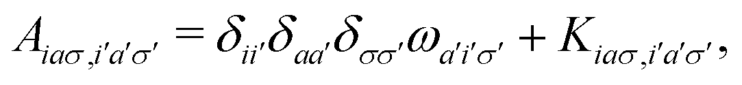

 , and, in the density matrix formulation, the coupling matrix elements are given by
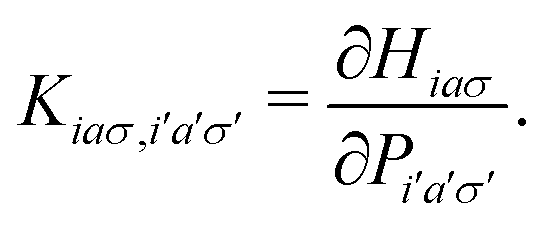


 and the position descriptors for electrons (POSe), holes (POSh) and excitons (POS), which are given by