
 Open Access Article
 This Open Access Article is licensed under a Creative Commons Attribution-Non Commercial 3.0 Unported Licence
Ultrasound-assisted sorption of Pb(II) on multi-walled carbon nanotube in presence of natural organic matter: an insight into main and interaction effects using modelling approaches of RSM and BRT†
Maryam Foroughiab,
Hassan Zolghadr Nasabc,
Reza Shokoohi *c,
Mohammad Hossein Ahmadi Azqhandid,
Azam Nadalic and
Ashraf Mazaheric
*c,
Mohammad Hossein Ahmadi Azqhandid,
Azam Nadalic and
Ashraf Mazaheric
aDepartment of Environmental Health, School of Health, Torbat Heydariyeh University of Medical Sciences, Torbat Heydariyeh, Iran
bHealth Sciences Research Center, Torbat Heydariyeh University of Medical Sciences, Torbat Heydariyeh, Iran
cDepartment of Environmental Health Engineering & Research Centre for Health Sciences, School of Public Health, Hamadan University of Medical Sciences, Hamadan, Iran. E-mail: reza.shokohi@umsha.ac.ir; shokoohia@yahoo.com; Tel: +98 38380026; Fax: +98 8138380509
dApplied Chemistry Department, Faculty of Gas and Petroleum (Gachsaran), Yasouj University, Gachsaran 75813-56001, Iran
First published on 24th May 2019
Abstract
In real-scale applications, where NPs are injected into the aqueous environment for remediation, they may interact with natural organic matter (NOM). This interaction can alter nanoparticles' (NPs) physicochemical properties, sorption behavior, and even ecological effects. This study aimed to investigate sorption of Pb(II) onto multi-walled carbon nanotube (MWCNT) in presence of NOM. The predominant behavior of the process was examined comparatively using response surface methodology (RSM) and boosted regression tree (BRT)-based models. The influence of four main effective parameters, namely Pb(II) and humic acid (HA) concentrations (mg L−1), pH, and time (min) on Pb removal (%) was evaluated by contributing factor importance rankings (BRT) and analysis of variance (RSM). The applicability of the BRT and RSM models for description of the predominant behavior in the design space was checked and compared using statistics of absolute average deviation (AAD), mean absolute error (MAE), root mean square error (RMSE), and multiple correlation coefficient (R2). The results showed that although both approaches exhibited good performance, the BRT model was more precise, indicating that it could be a powerful method for the modeling of NOM-presence studies. Importance rankings of BRT displayed that the effectiveness order of the studied parameters is pH > time > Pb(II) concentration > HA concentration. Although HA concentration showed the least effect in comparison with three other studied parameters theoretically, the experimental results revealed that Pb(II) removal is enhanced in presence of HA (73% vs. 81.77%), which was confirmed by SEM/EDX analyses. Hence, maximum removal (R% = 81.77) was attained at an initial Pb(II) concentration of 9.91 mg L−1, HA concentration of 0.3 mg L−1, pH of 4.9, and time of 55.2 min.
1. Introduction
The increase of heavy metal contamination in environmental matrices originating from industrial wastewater discharges, such as metal electroplating facilities, mining operations, fertilizer industries, tanneries, etc., has received great attention. The concerns are mainly their non-biodegradable nature, tendency to accumulate in living organisms, and toxicity and carcinogenicity.1 Among metals of particular concern,2 lead (Pb(II)) is categorized as a prevalent toxic metal and can easily enter the food chain via either drinking water or crop irrigation. It accumulates in vital body organs such as bones, muscles, liver, kidney, and brain. Excessive lead results in mental retardation, kidney problems, anemia, and severe damage to the nervous system, reproductive system, liver, and brain and causes sickness, sterility, abortion, stillbirths, and neonatal deaths.3 The maximum contaminant level (MCL) and maximum contaminant level goal (MCLG) established by the USEPA for lead are 0.015 mg L−1 and zero, respectively.4 In industrial wastewaters, Pb(II) concentrations can reach 200–500 mg L−1, which exceed water quality standards and must be reduced to 0.05–0.10 mg L−1 before release into aqueous ecosystems or sewage facilities.5Thus, efficient removal of heavy metals from water bodies is still a challenging task facing environmental engineers. Among developed remediation technologies for heavy metals, including chemical precipitation, ion exchange, adsorption, membrane separation, and electrochemical processes,6 adsorption is still known as one of the most efficient approaches and many adsorbents have been studied in recent decades.7–9 Among introduced adsorbents, carbon nanotubes (CNTs) have attracted considerable research attention due to their highly porous and hollow structure, large specific surface area, light mass density, and capability to establish strong electrostatic interaction with various kinds of pollutant molecules. These features have led to CNTs seeming a very promising candidate for adsorption of various kinds of pollutants from wastewater, including heavy metal ions.10,11 Depending on both CNT and solution chemistry, the apparent adsorption capacity for Pb(II) has been reported from several mg g−1 to about 100 mg g−1.12
However, in real-scale applications where the nanoparticles (NPs) are injected into the aqueous environment for remediation, interaction with natural organic matter (NOM) may occur. Hence, it is crucial to study the adsorption behavior of heavy metals by NPs in the absence or presence of NOM. NOM is one of the most abundant materials on earth and ubiquitously present in natural water bodies at concentrations ranging from a few mg L−1 to a few hundred mg L−1.13 Interaction between NOM and NPs can alter the physicochemical properties, sorption behavior, and even ecological effects of the adsorbents.14 For this reason, in many studies, NOM has been introduced into the process to investigate its effect on NPs performance in sorption of a target pollutant. Therefore, in recent years, growing numbers of studies have reported the effects of NOM on heavy metals removal by CNTs.15
However, all have focused on the investigation using the one-variable-at-a-time (OVAT) approach, in which the impacts of the main effective parameters are presented individually. This strategy suffers from not showing the interactions between all contributing variables. Multivariate statistical strategies have been preferred to the OVAT approach to identify the optimal combination of parameters and interactions between variables, improve cost- and time-effectiveness, develop a mathematical model, forecast the response, assess the model adequacy, and determine the optimal conditions for a given response.16,17 Response surface methodology (RSM) is known as an efficient procedure applicable not only to experimental design but also to development of a mathematical model (linear, square polynomial functions, etc.) for each response based on the obtained results.18 Boosted regression tree (BRT) model is a recently developed procedure for either multivariate classification or regression. This approach offers the benefits of both classical regression models and machine learning techniques. BRT adjusts complex linear and nonlinear responses to multiple categorical and continuous parameters even where the data suffer from collinearity-based challenges.19 Such tree-based methods were generally developed to optimize predictive performance by combining a large number of simple trees into a powerful model instead of considering a single tree based on conventional regression trees.20 These advantages led to application of RBT for the present study's modelling and optimization in addition to BBD strategy.
The objectives of this work were (i) to investigate the effect of NOM on MWCNTs in Pb(II) sorption by considering the parameters of Pb(II) and HA concentrations (mg L−1), pH, and time (min), (ii) to model the process and compute the impacts in terms of main effects and interactions using both RSM and BRT strategies and compare the results in terms of absolute average deviation (AAD), mean absolute error (MAE), root mean square error (RMSE), and multiple correlation coefficient (R2), and (iii) to introduce the optimal conditions of the process and the expected efficiency at such point. It should be emphasized that, although an increasing number of studies have been conducted in recent years to evaluate the effect of NOM on sorption-based processes of NPs, to the best of our knowledge none of them have investigated the process from modeling and/or interactions point of view. Therefore, this study highlighted the application and comparison of the RSM and BRT models on the process behavior.
2. Material and methods
2.1 Chemicals and instruments
All chemicals utilized in this research were reagent grade. The 100 mg L−1 stock solution of Pb(II) was achieved by dissolving an accurately weighed mass of Pb(NO3)2 (Merck, Germany) in deionized water. Humic acid (HA, Sigma-Aldrich, Germany) was selected to represent NOM. HA stock solution (100 mg L−1) was achieved by dissolving 0.01 g of HA powder in alkaline distilled water (pH 9.0, adjusted with concentrated NaOH). The solution was then filtered through 0.45 μm Whatman paper, sealed with aluminum foil, and kept at 4 °C.21 Required daily concentrations of Pb(II) and HA were achieved by dilution of the corresponding stock solutions. The initial pH was adjusted with H2SO4 or NaOH (Merck-Millipore, USA) using HACH model sension1 pH meter. HA concentrations were measured spectrophotometrically (model 1700, HACH) at 254 nm. The wavelength was chosen after scanning HA solutions over the range 200–800 nm. Pb(II) was detected using a Metrohm computrace voltammetric analyzer (model 797 VA with Software Version 1.0, Metrohm, Switzerland). Multi-walled carbon nanotubes (MWCN) were purchased from a local company (Neutrino, Iran) with claimed length ∼20 μm, outer diameter 30–50 nm, purity > 95%, specific surface area 60 m2 g−1, ash < 1.5 wt%, electrical conductivity > 100 s cm−1, and tap density 0.22 g cm−3.2.2 Characterization of MWCNT
A scanning electron microscope coupled with an energy-dispersive X-ray microanalyzer (SEM/EDX, model) was used to study the surface morphology and surface elemental compositions of the MWCNTs.22 The adsorbent was also structurally and chemically characterized with X-ray diffraction (XRD, model). The pH value at the point of zero charge (pHpzc) of MWCNT was determined experimentally. For this purpose, 0.02 g of MWCNT was added to 10 mL of solutions with different initial pH values (2–10). The dispersions were stirred for 48 h and withdrawn supernatants were measured for final pH. The pHpzc was calculated by plotting the obtained pH against the initial pH. The point at which the two lines crossed is pHpzc.232.3 Experimental design, analyses, and protocol
| N = 2k(k − 1) + C0 | (1) |
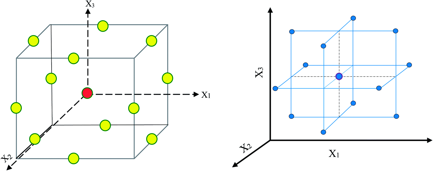 | ||
| Fig. 1 Design space at a three-level Box–Behnken approach. The yellow and red circles in the left scheme lie on the factorial and center points, respectively. | ||
According to eqn (1), a total of 29 experiments including 12 factorial points (Stds 1–25) and five replicates at the center points (Stds 25–29) were defined and their experimentally obtained results (summarized in Table 1) were used to describe the governed behavior in the process by fitting to the quadratic polynomial model presented in eqn (2).
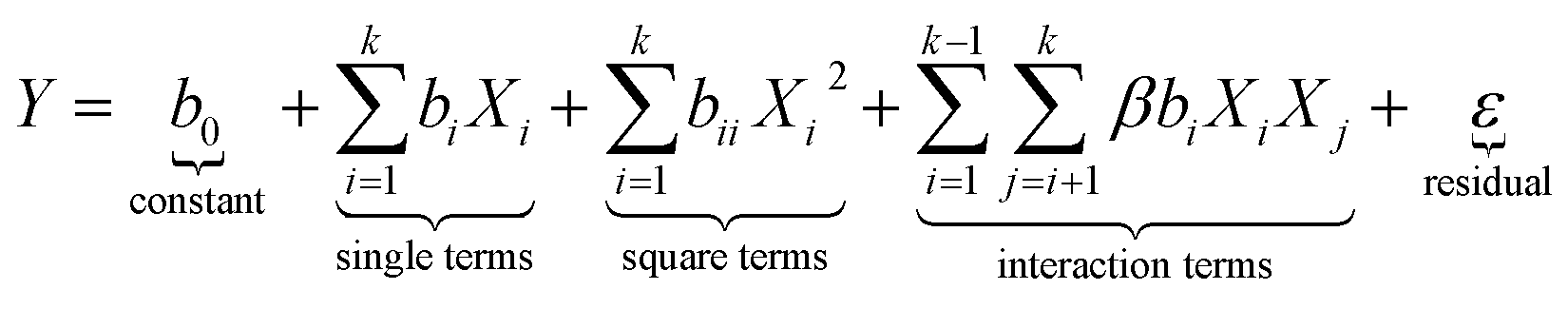 | (2) |
| Factor | Name | Units | Levels and ranges | ||
|---|---|---|---|---|---|
| Upper level (−1) | Middle (0) | Lower level (+1) | |||
| A | Pb concentration | mg L−1 | 2 | 6 | 10 |
| B | HA concentration | mg L−1 | 0 | 10 | 20 |
| C | pH | — | 3 | 5 | 7 |
| D | Time | min | 10 | 35 | 60 |
| Standard order | Run order | Leverage | Pb concentration (mg L−1) | HA concentration (mg L−1) | pH | Time (min) | Pb removal efficiency (%) | ||
|---|---|---|---|---|---|---|---|---|---|
| Actual value | Predicted value | Residual | |||||||
| 13 | 1 | 0.786 | 6 | 0 | 3 | 35 | 10.423 | 11.76 | −1.33 |
| 21 | 2 | 0.635 | 6 | 0 | 5 | 10 | 20.5018 | 16.56 | 3.94 |
| 6 | 3 | 0.647 | 6 | 10 | 7 | 10 | −8 | −9.42 | 1.42 |
| 9 | 4 | 0.619 | 2 | 10 | 5 | 10 | 58.23 | 60.02 | −1.79 |
| 28 | 5 | 0.2 | 6 | 10 | 5 | 35 | 23.8281 | 23.83 | −0.0052 |
| 8 | 7 | 0.704 | 6 | 10 | 7 | 60 | 23.5944 | 20.81 | 2.79 |
| 25 | 8 | 0.2 | 6 | 10 | 5 | 35 | 25.2748 | 23.83 | 1.44 |
| 11 | 9 | 0.645 | 2 | 10 | 5 | 60 | 47.645 | 46.86 | 0.7843 |
| 18 | 10 | 0.612 | 10 | 10 | 3 | 35 | 64.3901 | 60.34 | 4.05 |
| 4 | 12 | 0.648 | 10 | 20 | 5 | 35 | 61.362 | 60.51 | 0.8522 |
| 1 | 14 | 0.714 | 2 | 0 | 5 | 35 | 56.5768 | 57.77 | −1.19 |
| 22 | 15 | 0.758 | 6 | 20 | 5 | 10 | 39.394 | 37.72 | 1.68 |
| 24 | 16 | 0.67 | 6 | 20 | 5 | 60 | 21.7446 | 24.01 | −2.27 |
| 27 | 17 | 0.2 | 6 | 10 | 5 | 35 | 22.5867 | 23.83 | −1.25 |
| 19 | 18 | 0.656 | 2 | 10 | 7 | 35 | 38.7484 | 41.13 | −2.38 |
| 10 | 19 | 0.619 | 10 | 10 | 5 | 10 | 40.0267 | 42.15 | −2.12 |
| 5 | 20 | 0.597 | 6 | 10 | 3 | 10 | 26.1443 | 29.27 | −3.13 |
| 17 | 21 | 0.612 | 2 | 10 | 3 | 35 | 45.2172 | 41.71 | 3.5 |
| 29 | 22 | 0.2 | 6 | 10 | 5 | 35 | 22.0096 | 23.83 | −1.82 |
| 26 | 23 | 0.2 | 6 | 10 | 5 | 35 | 25.4672 | 23.83 | 1.63 |
| 14 | 24 | 0.786 | 6 | 20 | 3 | 35 | 41.0664 | 42.4 | −1.33 |
| 3 | 25 | 0.648 | 2 | 20 | 5 | 35 | 60.5635 | 59.49 | 1.07 |
| 2 | 26 | 0.714 | 10 | 0 | 5 | 35 | 61.362 | 62.78 | −1.42 |
| 12 | 27 | 0.645 | 10 | 10 | 5 | 60 | 71.2188 | 70.76 | 0.4561 |
| 20 | 28 | 0.656 | 10 | 10 | 7 | 35 | 26.7023 | 28.53 | −1.83 |
| 7 | 29 | 0.628 | 6 | 10 | 3 | 60 | 12.745 | 14.51 | −1.76 |
RF is an ensemble learning method for regression that consists of many decision trees and was first introduced by Tin Kam Ho of Bell Labs in 1995. The RF technique combines Breiman's “bagging” idea and the random collection of features. Several advantages have been reported for RF-derived models over other statistical approaches: they are able to handle missing values and high-dimensional data, recognize complex interactions among factors and the most important parameters measurements, and anticipate with high accuracy (low-bias models in addition to low-variation results) even for large databases.33 However, RF suffers from inherent limitations, such as overfitting for some datasets and unreliable variable importance scores, especially for categorical factors with different numbers of levels. These disadvantages can be overcome by employing boosting methods such as BRT.34 The process of BRT application includes fitting the model using random independent bootstrap replicates which are then combined by averaging the output for regression. In fact, BRTs are an ensemble strategy wherein many simple models are combined to improve the model performance (“boosting”) by means of recursive binary splits to related response to independent factors (regression trees). These approaches robustly factor collinearity, outliers, and missing data and can take both categorical and continuous parameters.35
So far, BRT approaches have been successfully used in different fields of chemistry with large data volumes, including reflectance spectroscopy,36 blood–brain barrier modelling,37 and cancer diagnostics.38 However, our literature survey shows that there is no evidence for use of BRT approach in the adsorption process from RSM data. It has been shown that the BRT model is one of the most powerful statistical approaches reported in science since the 1990s; the efficiency of BRT regression usually depends on three parameters: the number of trees (nt), tree complexity (tc), and learning rate (lr).39 However, the success of a BRT model relies on optimal sets of these regularization parameters. Hence, BRT models with various nt (1 to 100), tc (1, 4, 16) and lr (0.1, 0.25, 0.50, and 1.00) values were considered in the training to select the best BRT model with maximum R2 and minimum error.
2.4 Experimental producer (ultrasonic assisted removal procedure)
Ultrasonic-assisted adsorption experiments were conducted according to the matrix designed by BBD (Table 1) in a batch mode. For each run, a working solution with the desired concentration of Pb(II) and/or HA was prepared by dilution of the stocks, adjusting for pH using 0.1 M H2SO4 or NaOH. Then, 0.01 g of MWCNTs was added into 100 mL of the working solution in an aluminum foil-sealed flask. The flask was finally ultrasonicated at 40 Hz for a specific time interval. The adsorbent was then removed using 0.22 μm syringe filter and measured for Pb(II) concentration. The removal efficiency (%) was calculated as stated previously.40 The obtained data from this stage was used to develop the models.3. Results and discussion
3.1 Characterization of MWCNTs
The XRD pattern (Fig. S1†) showed that the MWCNTs were made of carbon. The peak position at 25.52° is a characteristic of hexagonal graphite and is attributed to the existence of tubular structure of carbon atoms with (002) planes. Moreover, the diffraction peak at 43.2° corresponded to the (100) planes of the nanotube structure.41The SEM images of MWCNTs and MWCNT/HA before and after Pb(II) sorption are shown in Fig. 2. As can be seen, the MWCNTs were smooth and free from impurities (Fig. 2a). The bulk morphology of the long particles is filament-like and oriented with uniform diameters, which indicates homogeneous MWCNTs. It can be seen from Fig. 2b (MWCNT/HA before adsorption of Pb(II)) that the extent of aggregation between MWCNTs in MWCNTs/HA was clearly reduced compared to raw MWCNTs, which can be attributed to hydrophobic and π–π attractions of HA with MWCNTs.42 The uniformly distributed MWCNTs/HA nanohybrid can greatly increase the surface-to-volume ratio and the efficiency of Pb(II) ion capture, thus greatly improving the removal properties of the prepared adsorbent.42 However, after the adsorption process, the tubes displayed swelling from the open ends of the MWCNTs (Fig. 2c). The functional groups (e.g. hydroxyl or carboxyl groups) created during the adsorption process will attach to these or to any other available defect sites. Therefore, the surfaces of MWCNTs after adsorption were less smooth in comparison with pristine MWCNTS, mainly due to the surface modification induced by adsorption.43
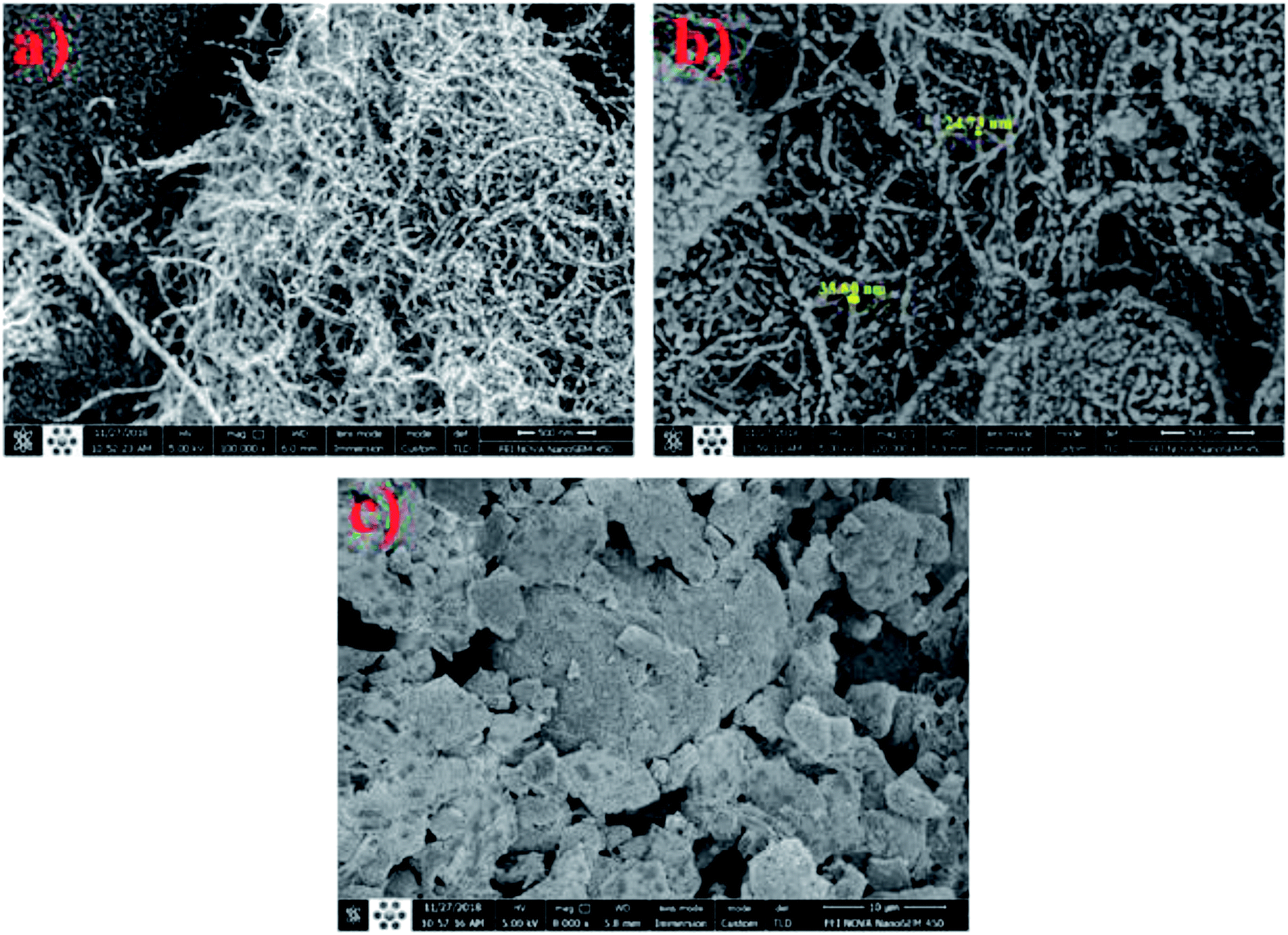 | ||
| Fig. 2 SEM images of pristine optimum MWCNTs (a) and MWCNTs/HA before (b) and after (c) adsorption of Pb(II). | ||
The sorption of Pb(II) was also confirmed by the comparison of EDX spectra of the MWCNTs before and after exposure to Pb(II)- and HA-containing solutions (Fig. S2†). In nanoparticles before sorption and those exposed to HA solution, no lead was detected, as can be seen from Figs. S2a and b,† whereas a sharp peak of lead appeared in the EDS spectrum of nanoparticles after the process (Fig. S2c†).
3.2 Analysis of BDD
ANOVA is a critical option for demonstration of model adequacy, in addition to showing the most important effects and interactions. The ANOVA results of Pb(II) removal by MWCNT in presence of HA are summarized in Table 2. From these, a semi-empirical expression for Pb(II) removal is given as eqn (3). The developed model was found to be significant at a 95% confidence interval as its F-value was 68.61. Table 2 revealed that the terms C (pH) and D (time) and the interaction effects of AC, AD, BC, BD, CD, A2, B2, and C2 were the significant model terms (P-value < 0.05). The F-value of lack of fit (LOF) was 6.01, implying there is a 5.12% chance that a LOF F-value this large could occur due to noise. Insignificant LOF confirms the suitability of the full quadratic model for forecasting the actual process behavior.| Pb removal (%) as coded form = 23.8333 + (1.50675 × A) + (−0.137164 × B) + (−8.09783 × C) + (3.86432 × D) + (−0.996687 × AB) + (−7.80475 × AC) + (10.4443 × AD) + (−15.4589 × BC) + (−10.7171 × BD) + (11.2484 × CD) + (30.1244 × A2) + (6.17927 × B2) + (−11.0312 × C2) + (0.989705 × D2). | (3) |
| Source | Sum of squares (SS) | df | Mean square | F-Value | p-Value | Status |
|---|---|---|---|---|---|---|
| a R2 = 0.9887, R2 adjusted = 0.9743, and R2 predicted = 0.9106, AP = 33.2441, and CV = 8.79. | ||||||
| Model | 9685.71 | 14 | 691.84 | 68.61 | <0.0001 | Significant |
| A-Pb | 27.24 | 1 | 27.24 | 2.70 | 0.1285 | |
| B-HA | 0.11 | 1 | 0.11 | 0.01 | 0.9178 | |
| C-pH | 587.40 | 1 | 587.40 | 58.26 | <0.0001 | |
| D-Time | 146.11 | 1 | 146.11 | 14.49 | 0.0029 | |
| AB | 3.97 | 1 | 3.97 | 0.39 | 0.5430 | |
| AC | 243.66 | 1 | 243.66 | 24.16 | 0.0005 | |
| AD | 436.33 | 1 | 436.33 | 43.27 | <0.0001 | |
| BC | 358.04 | 1 | 358.04 | 35.51 | <0.0001 | |
| BD | 273.59 | 1 | 273.59 | 27.13 | 0.0003 | |
| CD | 506.11 | 1 | 506.11 | 50.19 | <0.0001 | |
| A2 | 5416.76 | 1 | 5416.76 | 537.20 | <0.0001 | |
| B2 | 183.90 | 1 | 183.90 | 18.24 | 0.0013 | |
| C2 | 661.20 | 1 | 661.20 | 65.57 | <0.0001 | |
| D2 | 5.54 | 1 | 5.54 | 0.55 | 0.4743 | |
| Residual | 110.92 | 11 | 10.08 | |||
| Lack of fit | 101.29 | 7 | 14.47 | 6.01 | 0.0512 | Not significant |
| Pure error | 9.63 | 4 | 2.41 | |||
| Cor total | 9796.63 | 25 | ||||
The large R2 values (R2 = 0.9887, Radjusted2 = 0.9743, and Rpredicted2 = 0.9106) prove high correlation and agreement between the anticipated and obtained results. AP evaluates adequate model discrimination. In this study, the AP ratio of 33.24 indicates that the signal is sufficient to model.
3.3 Effect of the studied parameters
Of the studied parameters, pH was found to be the most effective factor. The effects of HA concentration, Pb concentration, time, and pH were found to be alternately positive and negative. The presence of NOM has shown a controversial effect on the pollution's sorption by different adsorbents. Although some studies reported a positive impact, others discuss the negative effects of NOM species on removal of different pollutants. Heavy metals' (ad)sorption by nano-based adsorbents in presence of NOM, however, showed an enhancement trend in almost all of the reports.44 As can be seen from Fig. 3c and eqn (3), HA presence could drastically enhance Pb(II) sorption. Despite the study of Tian et al.,14 who reported increased removal efficiency of Cd(II) only in high concentrations of HA (>10 mg L−1), the results of our work showed a positive effect in all the studied concentrations. This welcomed presence can result from the gradual binding of HA onto the sorption sites of the nanotube surfaces which were unfavorable for Pb(II). This fraction of CNT-bound HA could then improve the sorption of Pb(II). In fact, only a small portion of the “sorbed” carboxylic and phenolic groups of the macromolecular HA directly interact with the available surface sites on the nano material and the remaining fractions of the sorbed groups are free and ready to interact with the metal ion.45 The findings were also supported by EDX analyses. The enhancement of Pb(II) sorption onto the nanoparticles in the presence of HA can also be attributed to the existence of Mo and Co additions due to HA in the solution (Fig. S2b†). It is reported that Mo and Co residues in the HA-contacted MWCNTs can facilitate apparent Pb(II) sorption onto the adsorbent via formation of PbMoO4 precipitate between Pb(II) and MWCNTs-released MoO4.46 The elemental weight ratio of Mo/Co in the MWCNTs increased about ten-fold after Pb(II) sorption (Figs. S2b and c†), indicating Mo and Co were involved in the improvement. Mo was released into the solutions mainly as MoO42−, which could precipitate back on the sorbents via formation of PbMoO4, whereas Pb(II) could enhance the release of Co cations from the sorbents through ion exchange.46 In fact, the enhancement can be attributed to better Co exchangeability in the MWCNTs-HA complex than in MWCNTs alone. The negative effect of Pb(II) concentration would be attributed to occupation of achievable sites for the Pb species. At low initial concentration of Pb(II), most of the species will interact with the binding sites of either nanoparticles or HA-based available sites, resulting in higher percentage removal. At high initial concentrations, only some of the ions will combine with the limited available binding sites. In fact, the limitation of vacant sites on MWCNTs or provided by HA leads to the pollutant remaining in the solution at such concentrations.21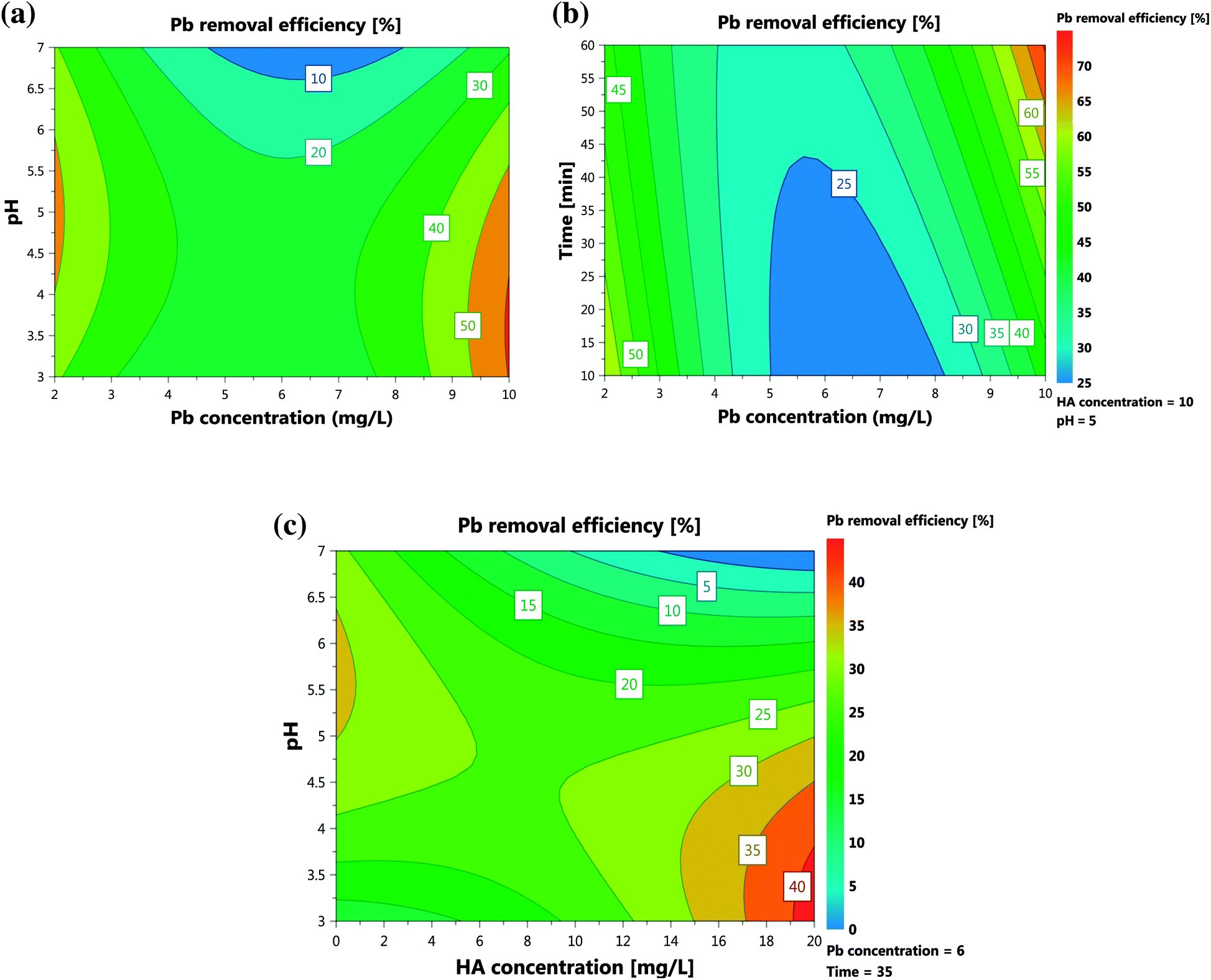 | ||
| Fig. 3 Response contour plots: effects of (a) initial Pb concentration and pH, (b) initial HA concentration and pH and (c) initial Pb concentration and time. | ||
Removal of Pb(II) was critically dependent on the solution pH value, which influences not only the surface charge of the MWCNTs but also the degree of ionization and speciation of the adsorbate. Fig. 3a shows that, with increase of pH from 3.0 to 5.0, the removal efficiency increased. The effect of pH can be simultaneously related to the following reasons: at pH = 3.0, adsorption effect is very weak as a result of the competition of H+ with Pb(II) on the adsorption sites; at pH = 5.0, the adsorption capability increases due to the role of functional groups on the MWCNTs surfaces; and at pH = 7.0, the adsorption capacity increases remarkably. The higher adsorption capacity of the NPs at pH 7.0 may also result from the cooperating roles of adsorption and precipitation. Since the pHpzc of NPs was found to be 6.32 (Fig. S3†), the removal efficiency would be expected to decrease because of the positive charges of MWCNTs at pH < pHpzc. However, in real experiments, we found that at lower pH values the efficiency increased. This may correspond to interactions of HA on the nano surface that prevent the expected phenomena. As pH increases, the weakly acidic HA with carboxylic and phenolic moieties turns to a more negatively charged species. Therefore, at higher pH values, repulsion of HA and MWCNTs increases, hindering further sorption of HA to MWCNTs. This results in a decreasing trend of removal at high pHs. Fig. 3c illustrates the sorption of HA on MWCNTs in terms of pH values. In fact, the improvement of HA sorption on the adsorbent, and therefore of Pb(II) removal, decreased with increasing pH values. The competition between Pb(II) and HA in occupation of active sites made their interaction insignificant as outlined by red in Fig. S4† (p-value = 0.54), while the interactions related to Pb(II) or HA with other parameters are all significant. In fact, such a plot visualizes the interaction between a pair of variables through the slope difference among them in relation to the response. When two variables' lines show a parallel trend, it is assumed that there is no interaction between their corresponding variables.40 As can be seen from Fig. S4,† except Pb(II) and HA concentrations, all the lines follow an unparallel trend, indicating interaction between them.
3.4 Analysis of BRT
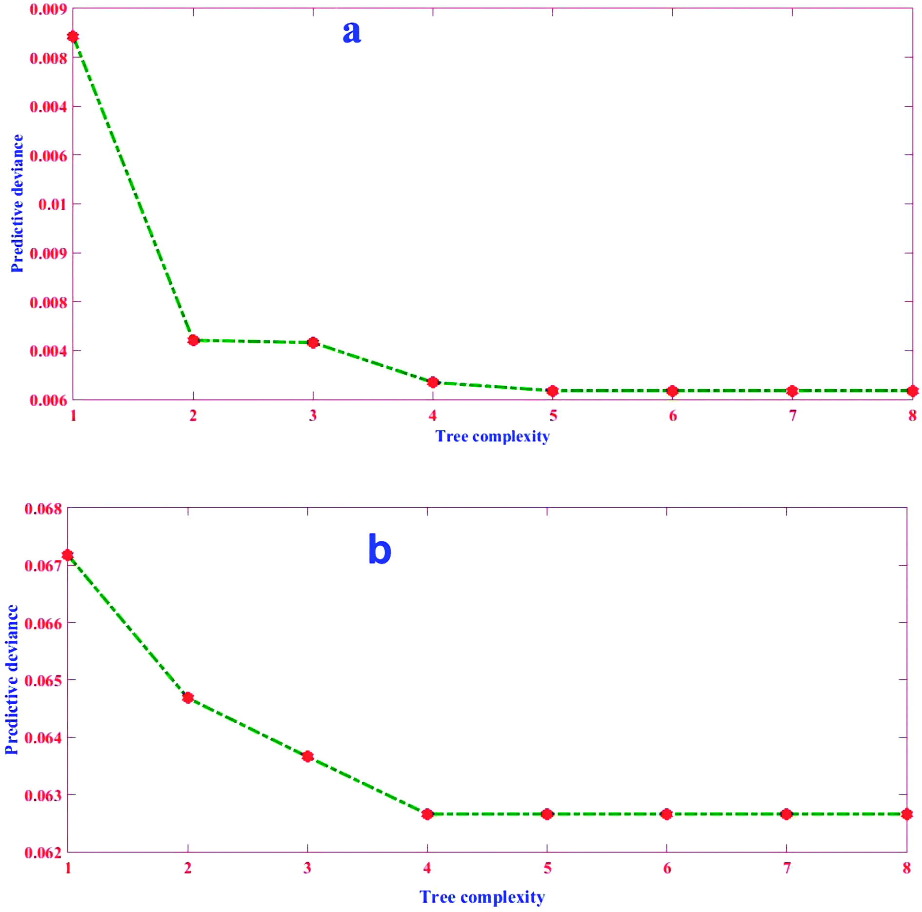
The good performance of the BRT model, as a function of prediction accuracy without overfitting, depends strongly on regularizing the boosted trees options and stopping tree growing parameters.47 Regularization process typically comprises optimizing three parameters, shrinkage or learning rate (lr), tree complexity (tc), and number of trees (nt), to obtain a balance between bias and variance.48 The lr represents the proportion of each successive tree to the ultimate model, as it proceeds via iterations.49 Although a small value of lr better minimizes loss function, it generally requires a larger number of nt to ensure sufficient convergence.50 Therefore, it is implemented by employing a small number, generally between 0.0001–0.1.48,51 The tc, also called the number of nodes (interactions) in each tree, controls the size of trees via contributing the interactions, if any, between variables. In fact, it determines the degree to which predictors may interact together regarding the response. More levels of interactions are explained with a higher tc.52 When tc = 1, each tree has a single decision stump and models the effect of one variable (i.e. only main effects are contributed in the model); when tc > 1, each tree fits a model that anticipates the interactions of factors (i.e., a maximum of two nodes in each branch) and so on.20 These above-mentioned parameters (i.e. lr and tc) control the nt that in turn is necessary to optimize predictive accuracy. To reflect the complexity between factors and utilize the strength of the BRT model, trees must be grown with higher levels of tree complexity. The success of a BRT model therefore depends on the optimal settings of the mentioned regularization parameters.48In this study, the nt (0–100) and lr in BRT method were obtained by a trial and error procedure for the datasets obtained from the BBD-introduced matrix. The optimal values were selected based on minimization of MSE at the tc of 1, 4, and 16 (Fig. 4).
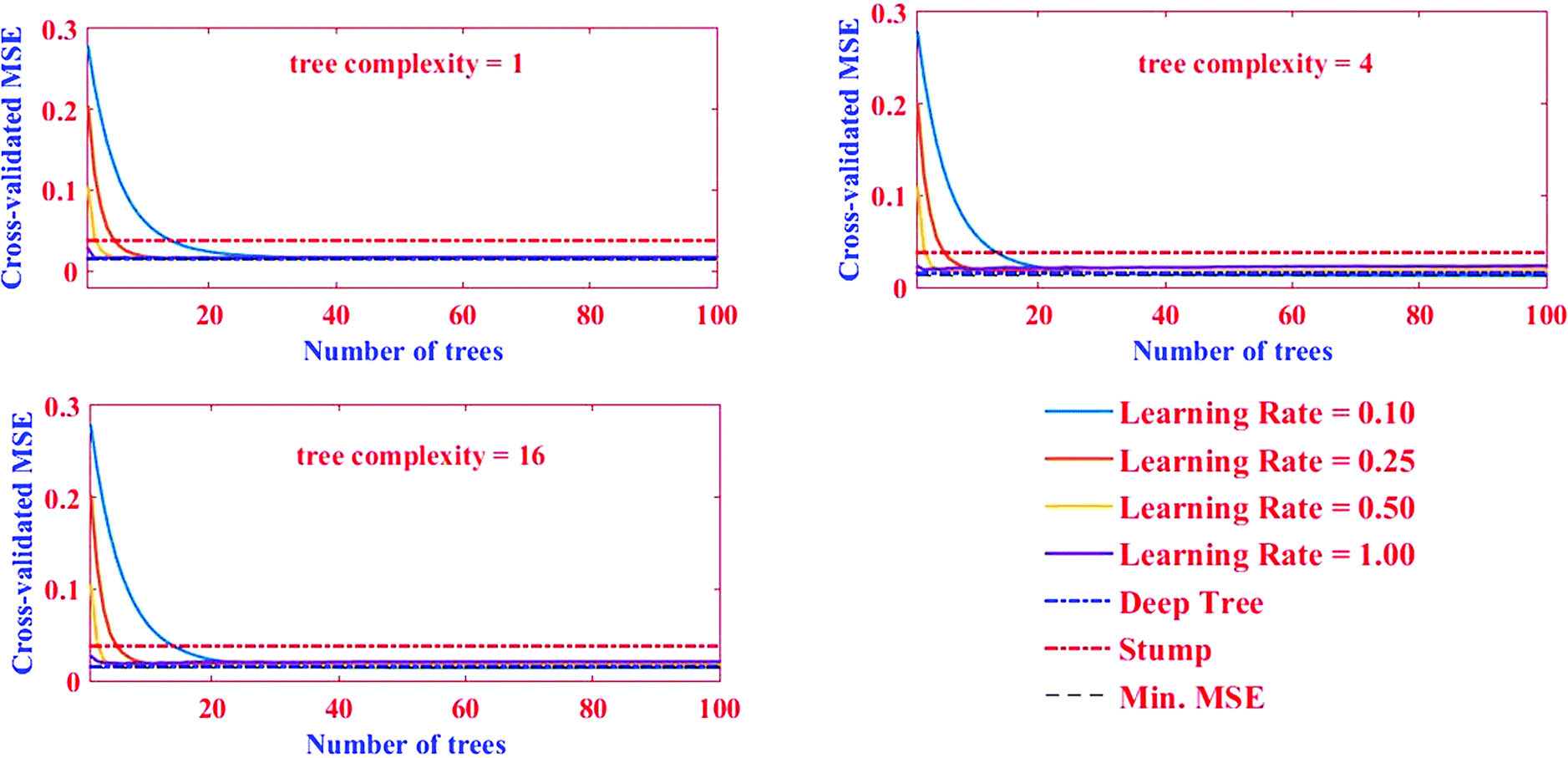 | ||
| Fig. 4 The association between the nt and the predictive deviance with four lr and three levels of tc. | ||
Herein, the aim was to achieve the combination of tree parameters, i.e. lr, tc, and nt, where a minimum MSE for the estimations of the response could be found. A value bigger than 1.00 for lr was not investigated because it was too fast and the derived minimum MSE would most probably be due to BRT overfitting. A similar phenomenon in lr = 1.00 and 0.5 were observed, namely that overfitting occurred but in relatively more trees (nt < 10). On the other hand, the smallest values for lr (i.e. 0.01 and 0.001) resulted in the best performance but needed thousands of trees to reach the minimum MSE (results for lr = 0.01 and 0.001 not shown). Elith et al. showed there was only slight improvement in the prediction power on a large number (N = 500) of trees.53 Nevertheless, researchers suggest the optimum lr must be selected to result in a minimum MSE value in the nt < 100 for different tc. The MSE as a function of tree complexity for lr = 0.1 for Pb removal is shown in Fig. 8. It can be seen from this figure that the optimum tc for both training and testing dataset is 4. The relative factor importance for each factor contributed is shown in Fig. 5. The relative importance of factors can be evaluated by averaging the number of times that a parameter is selected for splitting and the squared improvement resulting from these splits.54 As evident in Fig. 5, the maximum importance in Pb(II) removal by MWCNT is assigned to pH.
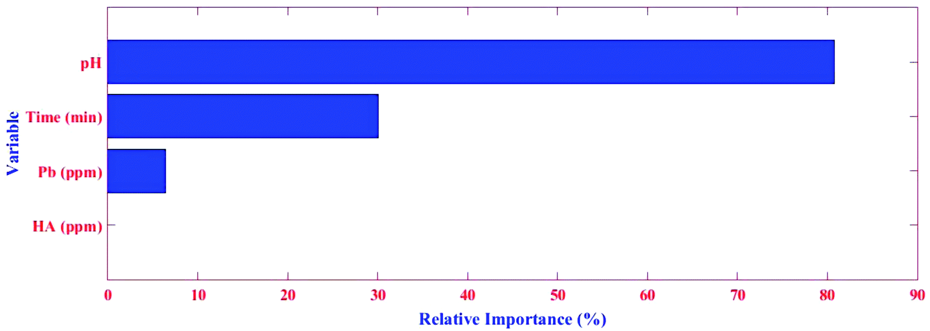 | ||
| Fig. 5 The relative importance of the variables in the BRT algorithms. | ||
As expected from sum of squares (SS, ANOVA results in Table 2), the pH and time were found to be the most effective parameters, with relative contributions of 75.00% and 19.35%, respectively, according to the BRT model for Pb(II) adsorption (Table 3). The concentrations of Pb(II) and HA had contributions of 4.00% and 1.650%, respectively, showing their insufficient influence on Pb(II) removal. The relative importance obtained from SS has good agreement with that achieved by BRT.
| Model | Input variable | |||
|---|---|---|---|---|
| Pb concentration (mg L−1) | HA concentration (mg L−1) | pH | Time (min) | |
| BRT | 4.00 | 1.65 | 75.00 | 19.35 |
| RSM | 3.95 | 1.50 | 75.35 | 19.20 |
3.5 Comparison BRT and RSM
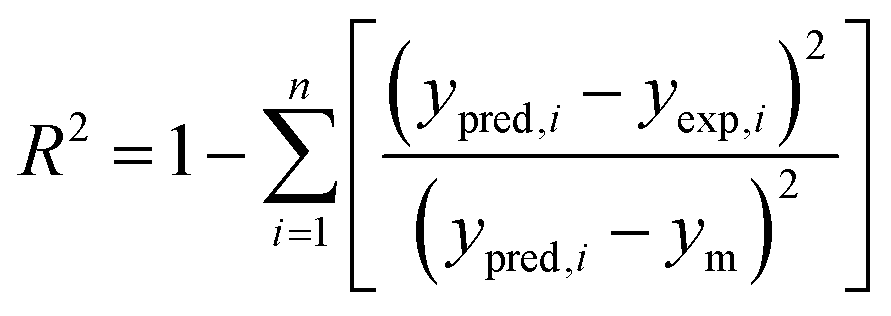
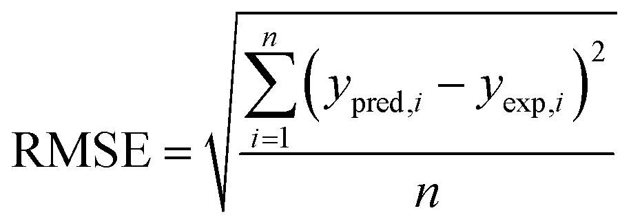
The performances of the RSM and BRT approaches for Pb(II) adsorption using MWCNTs were evaluated by comparing their corresponding residuals. Residuals are known as the differences between predicted responses and the obtained data. For this purpose, the residuals of both methods were comprised of RMSE, MAE, AAD, and R2, which are calculated by eqn (4)–(7).
 | (4) |
 | (5) |
 | (6) |
 | (7) |
R2 represents how well the developed equation truly fits to experimental data and is described by least-squares regression. It can be used for determining the degree of linear correlation of parameters in a regression calculation and a higher value implies more reliable prediction of the model.30,55,56 AAD is the average absolute deviation from a middle point and is considered a direct way to measure deviations between predicted and obtained results and, in contrast with R2, a smaller value is better.57 Mean square error (MSE) and RMSE are other statistics to check the quality of a model which are positive values and are preferred to be smaller and closer to zero. For a best-fitted model, sum of squared residuals, and therefore MSE and RMSE, should be minimum. The values for the mentioned statistics are listed in Table 4.
| Model | Statistical metrics (for TCS) | |||
|---|---|---|---|---|
| R2 | RMSE | MAE | AAD% | |
| BRT | 0.999889 | 0.006464 | 0.005755 | 1.217286 |
| RSM | 0.9887 | 0.022771 | 0.007659 | 1.679938 |
The plot of observed responses versus predicted ones can be informative respecting model fitting to a data set.58 The goodness-of-fit between the mentioned responses given by the RSM and BRT models are presented in Fig. 6. As is clear from Fig. 6, there is good agreement between the obtained responses and the predicted values in both models, especially in the case of BRT (R2 = 0.999889). In an adequate model, in addition, no major trend would be seen for the residuals against time or any other parameters.59 The plot of the internally studentized residuals versus the experimental runs is depicted in Fig. 7 and the residuals appear to behave randomly, suggesting their independence from experimental runs.
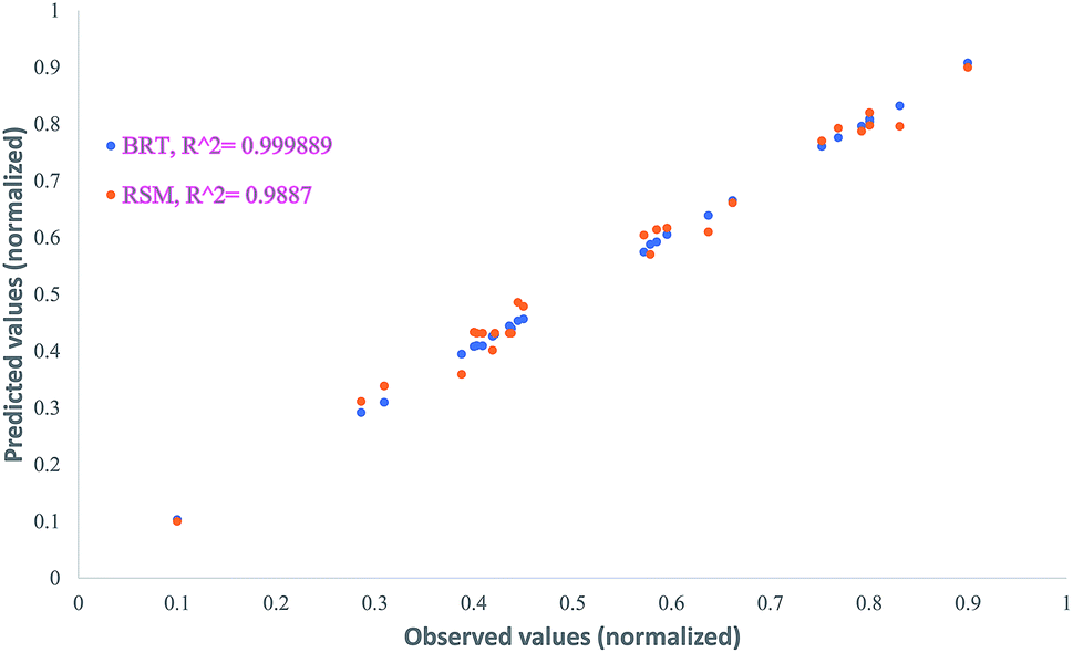 | ||
| Fig. 6 Distribution of the observed vs. predicted responses for RSM and BRT. | ||
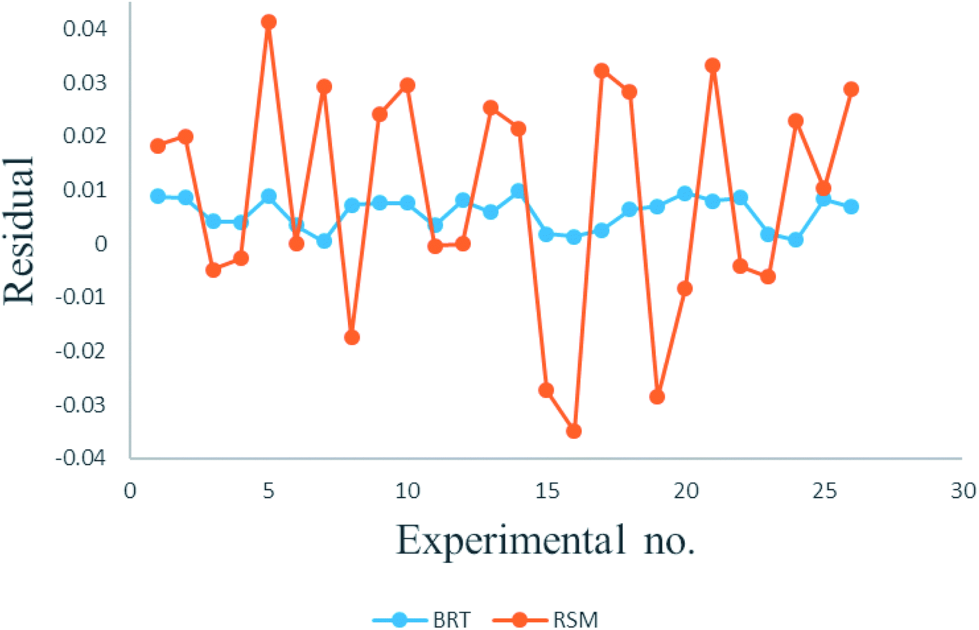 | ||
| Fig. 7 Distribution of the observed vs. predicted residuals for RSM and BRT. | ||
 | ||
| Fig. 8 MSE in terms of tree complexity for lr = 0.1: (a) training and (b) testing. | ||
Although both models presented appropriate statistics, the BRT model is superior to that developed by BBD from fitness and estimation capability point of views. However, RSM is still advantageous to its studied counterpart due to showing the experimental factors' influence as main effects or interactions and giving a regression equation on a process behavior in the studied design space.59
4. Conclusion
The main purpose of this study was to develop a novel model that could accurately and reliably both describe and predict the effect of NOM on Pb(II) removal by MWCNTs. Four main effective parameters (e.g. pH, HA and Pb(II) initial concentrations, and contact time) were studied under the designed experiments by BBD approach. BRT and RSM models were developed to forecast the removal of Pb(II) in the presence of HA as a NOM representative. The performances of the two developed models were then compared using the statistics of RMSE, R2, MAE, and AAD and analysis of the residuals. The results showed that, although both models satisfactorily predicted the adsorption of Pb(II) by MWCNTs from aqueous media, owing to RMSE = 0.022771, R2 = 0.999889, MAE = 0.005755, and AAD = 1.217286, the BRT model was much more accurate in its description of the predominant behavior in the process.Moreover, importance ranking for BRT displayed that pH and time are the most effective factors, with relative contributions of 75.00% and 19.35%, followed by Pb(II) and HA concentrations at 4.00% and 1.650%, respectively. Although HA concentration showed the least effect in comparison with three other studied parameters, the experimental results revealed that Pb(II) removal is enhanced in presence of HA (73% vs. 81.77%), which was confirmed by SEM/EDX analyses. Therefore, it seems that even though RSM is the most widely applied technique for optimization adsorption-based studies, the BRT approach can give more accurate and reliable results even with a smaller data set.
The findings of this work are potentially significant for evaluation of a treatment method along with the modeling capability. The BRT strategy is more appropriate due to taking much less computational time and handling a smaller number of contributing factors. However, as the bagging and boosting approaches are meta-algorithms, they can be employed with different kinds of trees or other regression models. The optimal situation and relative importance of each parameter for Pb(II) adsorption were determined and presented.
Conflicts of interest
There is no conflicts of interest declared by the authors.Acknowledgements
This project was financially supported by Hamadan University of Medical Sciences (grant no. 9309114367).References
- F. Fu and Q. Wang, J. Environ. Manage., 2011, 92, 407–418 CrossRef CAS PubMed.
- M. Khiadani, M. Zarrabi and M. Foroughi, J. Environ. Health Sci. Eng., 2013, 11, 43 CrossRef PubMed.
- G. D. Vuković, A. D. Marinković, S. D. Škapin, M. Đ. Ristić, R. Aleksić, A. A. Perić-Grujić and P. S. Uskoković, Chem. Eng. J., 2011, 173, 855–865 CrossRef.
- J. K. Edzwald, Water quality & treatment: a handbook on drinking water, McGraw-Hill, New York, 2011 Search PubMed.
- M. Arbabi, S. Hemati and M. Amiri, Int. J. Epidemiol. Res., 2015, 2, 105–109 Search PubMed.
- M. Hua, S. Zhang, B. Pan, W. Zhang, L. Lv and Q. Zhang, J. Hazard. Mater., 2012, 211, 317–331 CrossRef PubMed.
- L. Zeng, Y. Chen, Q. Zhang, X. Guo, Y. Peng, H. Xiao, X. Chen and J. Luo, Carbohydr. Polym., 2015, 130, 333–343 CrossRef CAS PubMed.
- A. R. Rahmani, M. Foroughi, Z. Noorimotlagh and S. Adabi, Avicenna J. Environ. Health Eng., 2016, 3, 1–6 Search PubMed.
- Z. Noorimotlagh, R. Darvishi Cheshmeh Soltani, G. Shams Khorramabadi, H. Godini and M. Almasian, Desalin. Water Treat., 2016, 57, 1684–1692 CrossRef CAS.
- X. Ren, C. Chen, M. Nagatsu and X. Wang, Chem. Eng. J., 2011, 170, 395–410 CrossRef CAS.
- Z. Noorimotlagh, S. A. Mirzaee, S. S. Martinez, S. Alavi, M. Ahmadi and N. Jaafarzadeh, Chem. Eng. Res. Des., 2019, 141, 290–301 CrossRef CAS.
- D. Lin, X. Tian, T. Li, Z. Zhang, X. He and B. Xing, Environ. Pollut., 2012, 167, 138–147 CrossRef CAS PubMed.
- J. Chen, Z. Xiu, G. V. Lowry and P. J. Alvarez, Water Res., 2011, 45, 1995–2001 CrossRef CAS PubMed.
- X. Tian, T. Li, K. Yang, Y. Xu, H. Lu and D. Lin, Chemosphere, 2012, 89, 1316–1322 CrossRef CAS PubMed.
- W.-W. Tang, G.-M. Zeng, J.-L. Gong, J. Liang, P. Xu, C. Zhang and B.-B. Huang, Sci. Total Environ., 2014, 468–469, 1014–1027 CrossRef CAS PubMed.
- M. Foroughi, A. R. Rahmani, G. Asgari, D. Nematollahi, K. Yetilmezsoy and M. R. Samarghandi, Fresenius Environ. Bull., 2018, 27, 1914–1922 CAS.
- M. Foroughi, S. Chavoshi, M. Bagheri, K. Yetilmezsoy and M. T. Samadi, J. Mater. Cycles Waste Manage., 2018, 20, 1999–2017 CrossRef CAS.
- M. Roosta, M. Ghaedi, A. Daneshfar and R. Sahraei, Spectrochim. Acta, Part A, 2014, 122, 223–231 CrossRef CAS PubMed.
- W. Zhang, Z. Du, D. Zhang, S. Yu and Y. Hao, Sci. Total Environ., 2016, 553, 366–371 CrossRef CAS PubMed.
- R.-M. Yang, G.-L. Zhang, F. Liu, Y.-Y. Lu, F. Yang, F. Yang, M. Yang, Y.-G. Zhao and D.-C. Li, Ecol. Indic., 2016, 60, 870–878 CrossRef CAS.
- M. H. A. Azqhandi, M. Foroughi and E. Yazdankish, J. Colloid Interface Sci., 2019, 551, 195–207 CrossRef CAS PubMed.
- R. Darvishi Cheshmeh Soltani, G. Shams Khoramabadi, H. Godini and Z. Noorimotlagh, Desalin. Water Treat., 2015, 56, 2551–2558 CrossRef.
- T. R. Bastami and M. H. Entezari, Chem. Eng. J., 2012, 210, 510–519 CrossRef CAS.
- A. Witek-Krowiak, K. Chojnacka, D. Podstawczyk, A. Dawiec and K. Pokomeda, Bioresour. Technol., 2014, 160, 150–160 CrossRef CAS PubMed.
- A. T. Nair and M. M. Ahammed, J. Cleaner Prod., 2015, 96, 272–281 CrossRef CAS.
- M. Mourabet, A. El Rhilassi, H. El Boujaady, M. Bennani-Ziatni, R. El Hamri and A. Taitai, Appl. Surf. Sci., 2012, 258, 4402–4410 CrossRef CAS.
- K. A. M. Said and M. A. M. Amin, J. Appl. Sci. Process Eng., 2016, 2, 8–17 Search PubMed.
- E. Solaymani, M. Ghaedi, H. Karimi, A. Azqhandi, M. Hossein and A. Asfaram, Applied Organometallic Chemistry, 2017 Search PubMed.
- M. Ghaedi, M. H. A. Azqhandi and A. Asfaram, Phys. Chem. Chem. Phys., 2017, 11299–11317 Search PubMed.
- A. Asfaram, M. Ghaedi, M. A. Azqhandi, A. Goudarzi and M. Dastkhoon, RSC Adv., 2016, 6, 40502–40516 RSC.
- M. A. Azqhandi, M. Ghaedi, F. Yousefi and M. Jamshidi, J. Colloid Interface Sci., 2017, 278–292 CrossRef PubMed.
- M. Ahmadi Azqhandi, M. Shekari and B. Ghalami-Choobar, Appl. Organomet. Chem., 2018, e4410 CrossRef.
- S. S. Matin, J. C. Hower, L. Farahzadi and S. C. Chelgani, Int. J. Miner. Process., 2016, 155, 140–146 CrossRef CAS.
- H. Mazaheri, M. Ghaedi, M. A. Azqhandi and A. Asfaram, Phys. Chem. Chem. Phys., 2017, 19, 11299–11317 RSC.
- R. Hale, S. Marshall, K. Jeppe and V. Pettigrove, Aquat. Toxicol., 2014, 152, 66–73 CrossRef CAS PubMed.
- B. Minasny and A. B. McBratney, Chemom. Intell. Lab. Syst., 2008, 94, 72–79 CrossRef CAS.
- E. Deconinck, M. H. Zhang, D. Coomans and Y. V. Heyden, J. Chemom., 2007, 21, 280–291 CrossRef CAS.
- Y. Qu, B.-L. Adam, Y. Yasui, M. D. Ward, L. H. Cazares, P. F. Schellhammer, Z. Feng, O. J. Semmes and G. L. Wright, Clin. Chem., 2002, 48, 1835–1843 CAS.
- T. Hastie, R. Tibshirani and J. Friedman, The Elements of Statistical Learning: Data Mining, Inference, and Prediction, Springer New York, 2013 Search PubMed.
- M. Foroughi, H. R. S. Arezoomand, A. R. Rahmani, G. Asgari, D. Nematollahi, K. Yetilmezsoy and M. R. Samarghandi, Korean J. Chem. Eng., 2017, 34, 2299–3008 Search PubMed.
- T. Al Mgheer and F. H. Abdulrazzak, Front. Nanosci. Nanotechnol., 2016, 2, 155–158 Search PubMed.
- X. Wang, S. Tao and B. Xing, Environ. Sci. Technol., 2009, 43, 6214–6219 CrossRef CAS PubMed.
- N. M. Mubarak, J. N. Sahu, E. C. Abdullah and N. S. Jayakumar, J. Environ. Sci., 2016, 45, 143–155 CrossRef PubMed.
- W.-W. Tang, G.-M. Zeng, J.-L. Gong, J. Liang, P. Xu, C. Zhang and B.-B. Huang, Sci. Total Environ., 2014, 468–469, 1014–1027 CrossRef CAS PubMed.
- Z. Niu, Q. Fan, W. Wang, J. Xu, L. Chen and W. J. A. R. Wu, Appl. Radiat. Isot., 2009, 67, 1582–1590 CrossRef CAS PubMed.
- D. Lin, X. Tian, T. Li, Z. Zhang, X. He and B. Xing, Environ. Pollut., 2012, 167, 138–147 CrossRef CAS PubMed.
- S. Shataeea, H. Weinaker and M. Babanejad, Procedia Environ. Sci., 2011, 7, 68–73 CrossRef.
- D. Saha, P. Alluri and A. Gan, Accid. Anal. Prev., 2015, 79, 133–144 CrossRef PubMed.
- A. Jafari, H. Khademi, P. A. Finke, J. Van de Wauw and S. Ayoubi, Geoderma, 2014, 232–234, 148–163 CrossRef.
- Y. Xia, C. Liu, Y. Li and N. Liu, Expert Syst. Appl., 2017, 78, 225–241 CrossRef.
- L. Vidal, L. Antúnez, A. Rodríguez-Haralambides, A. Giménez, K. Medina, E. Boido and G. Ares, Food Res. Int., 2018, 112, 25–37 CrossRef CAS PubMed.
- Y. L. Cheong, P. J. Leitão and T. Lakes, Spatial and Spatio-temporal Epidemiol., 2014, 10, 75–84 CrossRef PubMed.
- J. Elith, J. R. Leathwick and T. Hastie, J. Anim. Ecol., 2008, 77, 802–813 CrossRef CAS PubMed.
- J. T. Froeschke and B. F. Froeschke, Fish. Res., 2011, 111, 131–138 CrossRef.
- M. Arabloo, H. Ziaee, M. Lee and A. Bahadori, J. Taiwan Inst. Chem. Eng., 2015, 50, 123–130 CrossRef CAS.
- F. Kaytez, M. C. Taplamacioglu, E. Cam and F. Hardalac, Int. J. Electr. Power Energy Syst., 2015, 67, 431–438 CrossRef.
- A. Asfaram, M. Ghaedi, M. H. A. Azqhandi, A. Goudarzi and S. Hajati, J. Ind. Eng. Chem., 2017, 54, 377–388 CrossRef CAS.
- E. Solaymani, M. Ghaedi, H. Karimi, M. H. Ahmadi Azqhandi and A. Asfaram, Appl. Organomet. Chem., 2017, 31, 1–12 CrossRef.
- S. Porhemmat, M. Ghaedi, A. R. Rezvani, M. H. A. Azqhandi and A. A. Bazrafshan, Ultrason. Sonochem., 2017, 38, 530–543 CrossRef CAS PubMed.
Footnote |
| † Electronic supplementary information (ESI) available. See DOI: 10.1039/c9ra02881a |
| This journal is © The Royal Society of Chemistry 2019 |