
 Open Access Article
 This Open Access Article is licensed under a Creative Commons Attribution-Non Commercial 3.0 Unported Licence
Machine learning transferable atomic forces for large systems from underconverged molecular fragments†
Marius
Herbold
 a and
Jörg
Behler
*b
a and
Jörg
Behler
*b
aUniversität Göttingen, Institut für Physikalische Chemie, Theoretische Chemie, Tammannstraße 6, 37077 Göttingen, Germany. E-mail: marius.herbold@chemie.uni-goettingen.de
bLehrstuhl für Theoretische Chemie II, Ruhr-Universität Bochum, 44780 Bochum, Germany, and Atomistic Simulations, Research Center Chemical Sciences and Sustainability, Research Alliance Ruhr, 44780 Bochum, Germany. E-mail: joerg.behler@rub.de
First published on 29th March 2023
Abstract
Machine learning potentials (MLP) enable atomistic simulations with first-principles accuracy at a small fraction of the costs of electronic structure calculations. Most modern MLPs rely on constructing the potential energy, or a major part of it, as a sum of atomic energies, which are given as a function of the local chemical environments up to a cutoff radius. Since analytic forces are readily available, nowadays it is common practice to make use of both, reference energies and forces, for training these MLPs. This can be computationally demanding since often large systems are required to obtain structurally converged reference forces experienced by atoms in realistic condensed phase environments. In this work we show how density-functional theory calculations of molecular fragments, which are too small to provide such structurally converged forces, can be used to learn forces exhibiting excellent transferability to extended systems. The general procedure and the accuracy of the method are illustrated for metal–organic frameworks using second-generation high-dimensional neural network potentials.
1 Introduction
In recent years, machine learning potentials (MLPs)1–7 have become an important tool for atomistic simulations like molecular dynamics (MD) and Monte Carlo (MC), because they allow transfer of the accuracy of electronic structure calculations, most prominently density functional theory (DFT), to much larger systems containing thousands of atoms at a small fraction of the computational costs. Hence, the development of MLPs is a very active field of research and several generations have been proposed to date depending on the types of systems they can be applied to and the physical phenomena they are able to describe.8,9 Almost all MLPs applicable to large systems rely on atomic properties, which depend on the local environment up to a given cutoff radius Rc. As proposed in 2007 by Behler and Parrinello with the introduction of high-dimensional neural network potentials (HDNNP),10,11 in second-generation MLPs these properties are the atomic energies Ei of atoms i, which according to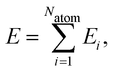 | (1) |
Nowadays, many types of second-generation MLPs are available, like various forms of neural network potentials,10,20–22 Gaussian approximation potentials (GAPs),23,24 moment tensor potentials (MTPs),25 spectral neighbor analysis potentials (SNAPs),26 atomic cluster expansion (ACE)27 and many others.28,29 They have been applied with great success to numerous systems, and to date they have remained the dominant type of MLP applied in large-scale simulations.
A consequence of the cutoff defining the local atomic environments is the possibility to use small systems accessible in electronic structure calculations for training MLPs. These can then be applied to simulations of much larger systems, which has been demonstrated, e.g., for metal clusters providing bulk properties,30,31 molecular fragments representing extended systems,32–34 and clusters of water molecules describing the liquid phase.35,36 This strategy does not only decrease the computational effort enabling the use of more accurate electronic structure methods but also reduces the complexity of the configuration space to be sampled to the energetically relevant degrees of freedom.
Still, the generation of the reference data is the most time-consuming part in the development of MLPs, and thus identifying the smallest possible systems which provide all required information about the atomic interactions, i.e., the potential-energy surface (PES), is of high interest. This is not only important for the generation of initial training sets but in particular also for the systematic improvement of MLPs by active learning.30,37–43 In the latter case the missing atomic environments are typically identified in production simulations, i.e., using systems which are often too large for the direct application of electronic structure methods. Consequently, strategies for reducing the systems to the most essential structural features still containing the required information are needed.
Nowadays it is common practice to employ energies and forces to train MLPs,30,44–46 which allows to extract a lot of information from electronic structure calculations. Several procedures have been proposed in the literature to determine the cutoff radius required for obtaining converged atomic forces. In a study on the development of a GAP for carbon, a statistical approach has been suggested in which the local environment of the atom of interest is frozen while the positions of the atoms outside the cutoff sphere are modified.47 For a sufficiently large cutoff radius there is only a negligible influence of these displacements on the variance of the forces of the central atoms.
Here, we build on an alternative approach making use of the Hessian, which provides the analytic derivatives of the forces.48 This method allows to identify the influence of each individual atom in the system on a given force of interest, and a rigorous procedure to determine the required reference system size can be established for a desired degree of force convergence. This system size can be expressed in terms of a converged fragment radius Rconvfrag including all neighboring atoms that have to be included for obtaining accurate forces in electronic structure calculations. If molecular or cluster fragments of this size are used, training of MLPs can be performed with forces numerically corresponding to those in much larger, condensed systems. Further details about this method can be found in ref. 48.
In the present work we show that the use of such converged fragments is not necessarily required for constructing MLPs and that it is possible to further decrease the size of the reference systems to about  . Assuming three-dimensional systems with a homogeneous distribution of atoms, the volume and thus the number of atoms can be reduced by approximately a factor of eight. This results in a drastic reduction of the computing time in electronic structure calculations, which often have a very unfavorable scaling with respect to system size.
Our approach is based on the insight that, as detailed below, the analytic atomic forces corresponding to the total energy expression eqn (1) depend on up to twice the cutoff radius defining the atomic energy contributions in MLPs.11 On the other hand, if converged electronic structure forces of bulk-like environments shall be learned directly, often large fragments with radii of about 8–12 Å are required in electronic structure calculations. Here we show that as a consequence of the relation between forces and atomic energies molecular fragments of only about half this radius (with a numerical value depending on the specific system) are sufficient to extract the relevant information needed to predict accurate MLP forces in systems of arbitrary size. This is possible although these small fragments, which fully define the atomic energies according to eqn (1), yield numerical reference forces strongly differing from the target forces in the condensed phase, since the atomic environments are incomplete with respect to the information needed to obtain bulk-like forces.
We illustrate our approach using the iso-reticular metal–organic framework IRMOF-1 (also called MOF-5), and generalize our findings by including also some data for the larger systems IRMOF-10 and IRMOF-16.49 MOFs are nanoporous, crystalline materials consisting of two parts – organic linker molecules, which interconnect inorganic secondary building units (SBUs) – with a large diversity of possible linker molecules and SBUs.49–53 The simulation of MOFs is a challenging task due to their often large unit cells. Furthermore, postsynthetic modifications50,54,55 and functionalizations50,56 increase the structural variety of MOFs. Hence, MOF properties can be designed for many different applications like gas storage, separation, catalysis and optical devices.50,56–59 Consequently, theoretical studies are of high interest for the analysis and prediction of MOF properties,60 and reliable and accurate interatomic potentials are urgently needed.61,62 Accordingly, several MLPs for MOFs have been reported in the literature to date.33,63,64
For our benchmark study, two types of HDNNPs are constructed based on either converged fragments providing bulk-like DFT reference forces, or making use of smaller fragments of about half this diameter yielding forces strongly differing from the bulk material. We show that in both cases HDNNPs of comparable quality can be obtained predicting reliable forces suitable for simulations of large systems.
2 Methods
In this work we demonstrate our approach using high-dimensional neural network potentials of the second generation.10,11 Starting from the total energy expression in eqn (1), the atomic energy contributions are provided as outputs of separate atomic feed-forward neural networks, which have the same architecture and set of numerical weight parameters for a given element. Accordingly, each element-specific atomic neural network has to be evaluated as many times as atoms of the respective chemical species are present in the system resulting in a close-to linear scaling of the method.The input vectors of the individual atomic neural networks consist of descriptors containing the structural information about the respective atomic environments up to the cutoff radius. They need to take into account the mandatory permutation, translation and rotation invariances of the atomic energies. In the present work atom-centered symmetry functions (ACSF) are used for this purpose,65 which smoothly decay to zero in value and slope at the cutoff radius.
In the iterative training process the weight parameters of the atomic neural networks are adjusted to accurately reproduce total energies and forces for a given reference data set obtained from electronic structure calculations. No energy partitioning is required in the process since the total potential energy is automatically distributed among the atoms during the weight optimization. Simultaneously, also the available force information can be used to optimize the weights, since the analytic forces depend on the same weight parameters as the atomic energies.
For HDNNPs, the atomic force components acting on atom A with respect to the Cartesian coordinate RαA with α = {x, y, z} are given by
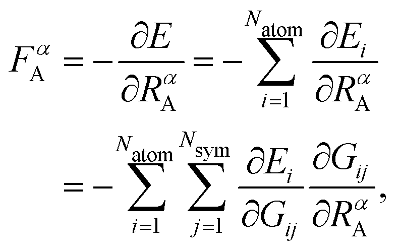 | (2) |
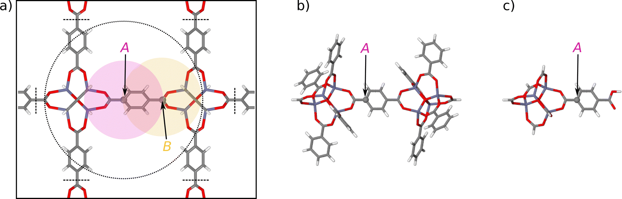 | ||
| Fig. 1 (a) Illustration of the environment-dependence of the atomic forces in bulk IRMOF-1. While the atomic energy EA of carbon atom A only depends on the positions of the neighboring atoms within a sphere of radius Rc (red circle), the force vector FA depends on all atomic positions in a sphere of radius of up to 2Rc (dotted circle). The reason for this extended range is the definition of the force as the negative derivative of the total energy, which according to eqn (2) consists of the derivatives of all atomic energies depending on the coordinates of atom A. Since in turn these atomic energies involve atoms as far as 2Rc from atom A (as shown by the yellow sphere of atom B). Atoms beyond twice the cutoff radius do not interact with atom A. Panel (b) shows a large molecular fragment (fragment radius Rconvfrag = 8.718 Å) providing converged DFT forces at the central atom A, closely approximating the forces in the periodic bulk system. The fragment has been constructed by removing all atoms beyond the dashed black lines shown in (a) following the procedure described in ref. 48. Panel (c) shows a much smaller fragment with about half fragment radius (Rfrag = 4.359 Å) containing only atoms within Rc. | ||
However, since according to eqn (2) the individual force components consist of the derivatives of the atomic energies, in principle it should be possible to derive the forces in extended bulk-like environments from atomic energies defined by all neighbors within Rc only. Therefore, training HDNNPs with information restricted to the close atomic environments within Rc only should be sufficient to describe the PES even in the condensed phase.
The procedure to derive such a HDNNP for a given system consists of several steps. First, DFT calculations can be used to determine Rconvfrag, i.e. the physical interaction range, providing converged bulk-like forces. Then, it is possible to derive the minimal cutoff 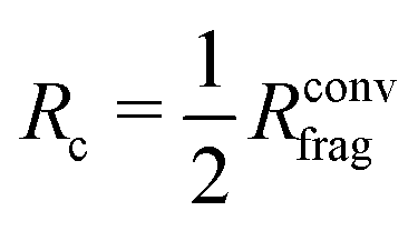 required in the HDNNP to define the atomic energies. DFT calculations for fragments of this reduced size can then be used to train a HDNNP. This HDNNP, which consequently has not been trained to fragments large enough to contain bulk-like forces, should then be transferable to extended systems. In the present work we will demonstrate this workflow for the case of metal–organic frameworks.
3 Computational details
All DFT calculations reported in this work have been carried out using the FHI-aims code68 (release version 171221). FHI-aims is an all-electron code employing a numerical atomic orbital basis, which is determined in free atom calculations. The RPBE functional69 has been employed to describe electronic exchange and correlation in combination with dispersion corrections according to the method of Tkatchenko and Scheffler.70 Furthermore, relativistic corrections were included by the atomic zero-order regular approximation (ZORA).68The DFT parameters were chosen to converge total energy differences to about 1 meV per atom. For all elements the basis set includes the FHI-aims recommended functions of the minimal basis, the functions of tier 1 and the first basis function of tier 2. The confinement potential has a width of 2 Å at the onset radius of 4 Å. The number of radial shells of the numerical integration grid corresponds to the element-specific tight settings. The angular integration grids and the atom-centered charge density expansion are equivalent to the light settings. For the calculations of the large periodic IRMOF bulk structure the Γ point has been used, while molecular fragments have been computed without periodic boundary conditions. The applied convergence criteria for the self-consistent calculations are 10−4, 10−2 eV, 10−6 eV and 10−2 eV Å−1 for the electron density, the energy eigenvalue sum, the total energy, and the atomic forces, respectively. For structural optimizations, the Broyden–Fletcher–Goldfarb–Shanno (BFGS) algorithm71 has been employed using an atomic force convergence criterion of 10−2 eV Å−1.
The HDNNPs have been trained using the program RuNNer11,66 employing two hidden layers containing 15 neurons each in the atomic neural networks. The hyperbolic tangent and a linear function have been used as activation functions for the hidden layers and the output node, respectively. The parameters of the ACSFs are given in the ESI.† A global extended Kalman filter has been applied for optimizing the weight parameters72 using reference energies and forces. The reference data set has been split in 90% training data set and 10% test data set.
The IRMOF structures investigated in this work (Fig. 2) contain the same zinc-oxo-cluster SBU and share the overall topology. The only difference is in the linker molecule, which is benzene-1,4-dicarboxylate (BDC) in IRMOF-1, biphenyl-4,4′ -dicarboxylate (BPDC) in IRMOF-10, and terphenyl-4,4′′-dicarboxylate (TPDC) in IRMOF-16. Initially, the atomic positions and lattice parameters of the IRMOF bulk structures have been optimized by DFT. The geometrically nonequivalent atoms of IRMOF-1, -10, and -16 are shown in the lower part of Fig. 2, and the initial training structures consist of molecular fragments cut from the bulk centered at these atoms. These fragments have then been saturated by hydrogen following the procedure described in ref. 48. Two different fragment radii have been employed as shown in Fig. 1b and c. The larger radius Rconvfrag = 8.718 Å corresponds to the converged radius providing bulk-like DFT forces with a maximum error of 0.125 eV Å as determined in ref. 48. and is equivalent to 2·Rc, while the smaller radius Rfrag = 4.359 Å corresponds to Rc. The value of Rconvfrag = 8.718 Å has been identified in previous work using an analysis of the DFT Hessian, which provides the second derivatives of the energies or the first derivatives of the energy gradients (negative forces) with respect to the atomic coordinates. This allows to decompose the Hessian into 3 × 3 submatrices containing the information about the dependence of a force vector on the Cartesian coordinate vector of any other atom. The norm of this Hessian submatrix then allows to quantify this interaction by a single number that can be related to the error in the force when truncating the system beyond the respective neighboring atom. For a series of model systems we found that this relation is rather universal and can be applied to determine the interaction range for a desired level of force convergence.
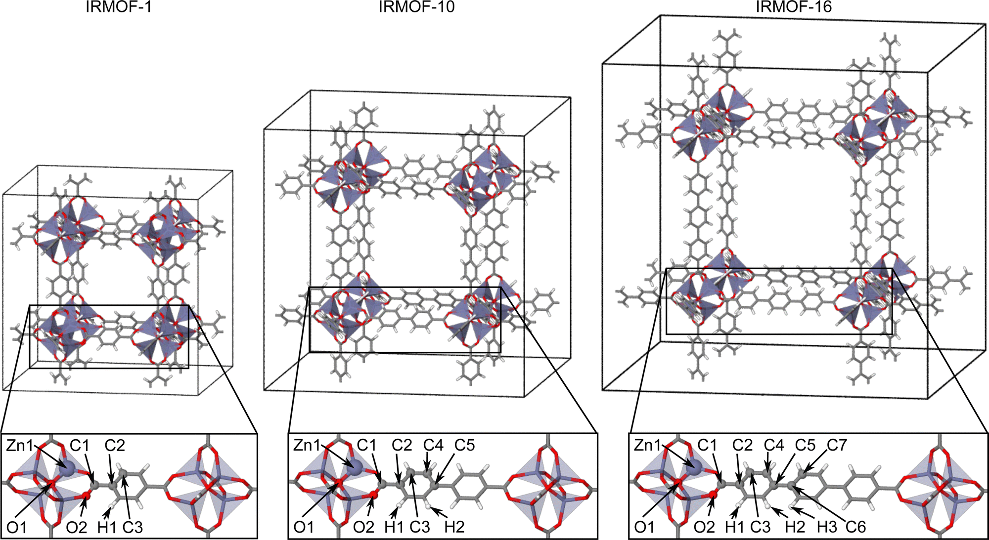 | ||
| Fig. 2 Bulk unit cells of IRMOF-1, -10, and -16 and definitions of the in-equivalent atomic sites in the lower panels. Atoms have been colored by element (zinc: violet, oxygen: red, carbon: grey, hydrogen: white). | ||
The required training structures have been generated initially by molecular dynamics simulations of the fragments in vacuum followed by active learning of bulk systems using the RuNNerActiveLearn tool.73,74 The second HDNNP required for the active learning has been constructed using 2 hidden layers containing 20 neurons per layer. Molecular dynamics simulations in the NPT ensemble (1 bar, 300–1000 K, 1 fs time step, 200 ps simulation time) employing preliminary potentials have been carried out with the n2p2 program package75 and the LAMMPS code76 to generate IRMOF bulk geometries, which have then been searched by active learning for structures with forces deviating substantially between different preliminary HDNNPs. The applied selection criterion has been a force deviation of 1 eV Å−1. Fragments have then been cut from the bulk centered at these atoms and included in the reference set. Moreover, atomic environments giving rise to extrapolations beyond the covered ACSF values have also been included in the data set.
4 Results and discussion
4.1 General strategy
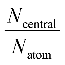
For the construction of the HDNNPs we have combined data for all three MOF systems. Three different setups have been used to investigate the role of the fragment radius of the DFT reference structures and of the symmetry function cutoff radius describing the atomic environments in the HDNNP:• HDNNP1 is based on DFT calculations of small molecular fragments with Rfrag = 4.359 Å only, which are too small to provide converged bulk-like forces. Due to this small size only a small cutoff Rc = 4.359 Å can be applied in the construction of the HDNNP, since otherwise the atomic environments of the central atoms would be incomplete inside their cutoff spheres. This incompleteness would result in extrapolations when applying the potential to large periodic systems. The molecular fragments centered at the nonequivalent atomic sites are shown in Fig. 3. The upper part of Table 1 contains a compilation of the number of atoms and the number of central atoms in complete environments within a sphere of radius Rc = 4.359 Å for all fragments. HDNNP1 is constructed to answer the question if small fragments are indeed sufficient to construct a potential for the condensed system.
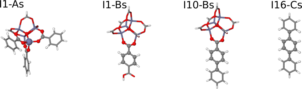 | ||
| Fig. 3 Small molecular fragments for IRMOF-1, -10, and -16 covering all nonequivalent atomic sites. The molecular fragment structures are represented by sticks, while the central atoms of the fragments embedded in a complete environment up to a radius of Rfrag = 4.359 Å are shown as balls. | ||
| Small fragments | ||||
|---|---|---|---|---|
| I1-As | I1-Bs | I10-Bs | I16-Cs | |
| N atom | 59 | 42 | 49 | 32 |
| N central | 17 | 11 | 17 | 16 |
|
0.29 | 0.26 | 0.35 | 0.5 |
| Extended large fragments | ||||||
|---|---|---|---|---|---|---|
| I1-A′ | I1-B′ | I10-A′ | I10-B′ | I16-B′ | I16-C′ | |
| N atom | 107 | 146 | 149 | 156 | 209 | 38 |
| N central | 65 | 62 | 101 | 68 | 161 | 24 |

|
0.61 | 0.42 | 0.68 | 0.44 | 0.77 | 0.63 |
• HDNNP2 is trained to large molecular fragments constructed using the radius Rconvfrag = 8.718 Å, which provide structurally converged DFT forces numerically corresponding to bulk forces in the condensed phase. The original fragments are shown in Fig. 4. Since several of these fragments exhibit a rather small number of bulk-like atoms with converged DFT forces, the fragments have been slightly extended as displayed in Fig. 5 to achieve a more favorable bulk atom-to-surface atom ratio (cf.Table 2). These extended fragments have finally been used for training HDNNP2. Still, the same small symmetry function cutoff Rc = 4.359 Å as in case of HDNNP1 is applied, which results in a rather large number of central atoms with complete environments within Rc as listed in the lower part of Table 1. HDNNP2 will allow to answer the question if a small cutoff radius is sufficient in combination with fully converged reference DFT forces to describe the bulk.
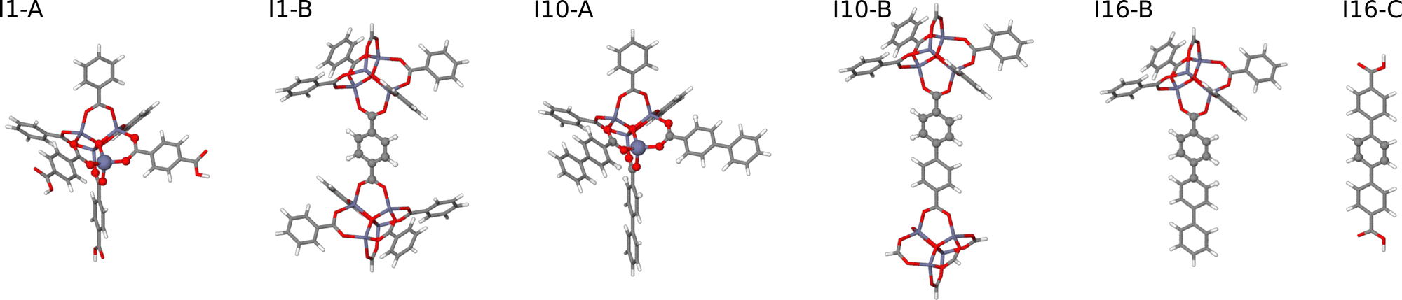 | ||
| Fig. 4 Large, size-converged molecular fragments of IRMOF-1, -10, and -16. The molecular fragment structures are represented by sticks, while the central atoms of the fragments embedded in a bulk-like environment up to a radius of Rconvfrag = 8.718 Å are shown as balls. | ||
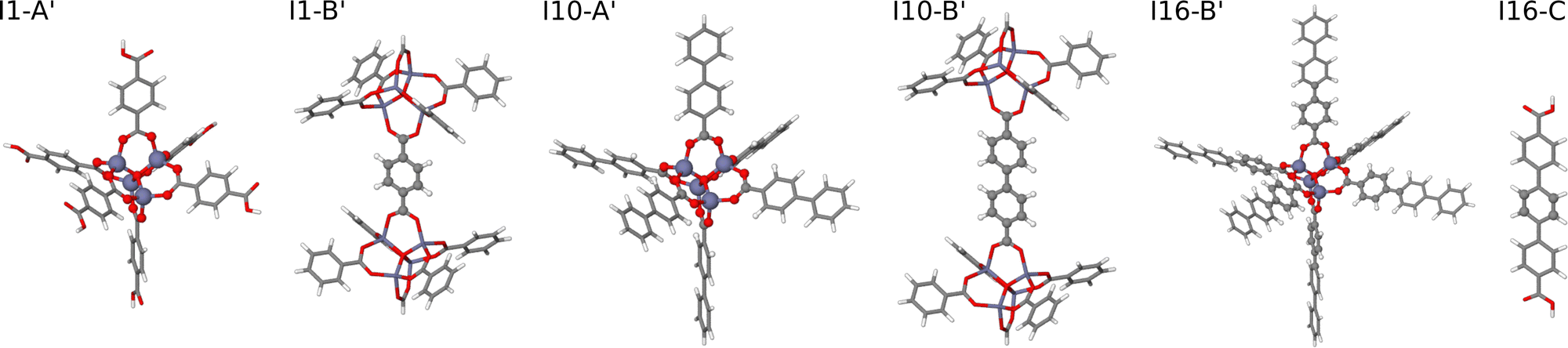 | ||
| Fig. 5 Extended large molecular fragments of IRMOF-1, -10, and -16 with an increased number of atoms in bulk-like environments. The molecular fragment structures are represented by sticks, while the central atoms of the fragments embedded in a bulk-like environment up to a radius of Rconvfrag = 8.718 Å are shown as balls. The fragments I1-B′ and I16-C′ are identical to their counterparts shown in Fig. 4. | ||
| Original large fragments | ||||||
|---|---|---|---|---|---|---|
| I1-A | I1-B | I10-A | I10-B | I16-B | I16-C | |
| N atom | 98 | 146 | 119 | 116 | 99 | 38 |
| N central | 8 | 12 | 17 | 11 | 14 | 4 |

|
0.08 | 0.08 | 0.14 | 0.09 | 0.14 | 0.11 |
| Extended large fragments | ||||||
|---|---|---|---|---|---|---|
| I1-A′ | I1-B′ | I10-A′ | I10-B′ | I16-B′ | I16-C′ | |
| N atom | 107 | 146 | 149 | 156 | 209 | 38 |
| N central | 17 | 12 | 35 | 22 | 101 | 4 |

|
0.16 | 0.08 | 0.23 | 0.14 | 0.48 | 0.11 |
• Finally, HDNNP3 is trained using the same extended, size-converged molecular fragments (Rconvfrag = 8.718 Å) as HDNNP2, but applying an increased symmetry function cutoff 2Rc = 8.718 Å such that all information required to compute numerically bulk-like forces using HDNNP3 is available. The number of central atoms embedded in complete environments with this extended cutoff is given in the bottom part of Table 2. HDNNP3 will serve as reference potential trained to converged DFT data making use of all structural information relevant for the DFT forces.
Our goal is now to investigate by comparing these HDNNPs, if the information content of the small molecular fragments, which fully define the atomic energies but not the forces in a bulk-like environment, is sufficient to accurately represent the PES of large condensed systems. In this case HDNNP1, HDNNP2 and HDNNP3 should be of similar quality, and the use of small fragments with a radius rigorously derived from DFT calculations48 would allow to drastically reduce the computational effort for the generation of the reference data. Our focus is on IRMOF-1, but also data of IRMOF-10 and IRMOF-16 is included to generalize our findings, although we do not aim to construct comprehensive PESs for atomistic simulations of these systems here.
4.2 High-dimensional neural network potentials
An initial training data set (“HDNNP1-initial”) has been generated from ab initio MD simulations at 600 K and a timestep of 1.5 fs for the four small fragment structures in vacuum (cf.Fig. 3), resulting in 3498 structures (I1-As: 682, I1-Bs: 908, I10-Bs: 908, I16-Cs: 1000) with their associated energies and forces. A first preliminary HDNNP represents this initial data with a good accuracy, exhibiting low root mean squared errors (RMSE) for the energies of the training (Etrain = 0.0012 eV atom−1) and test data set (Etest = 0.0013 eV atom−1), as well as acceptable errors for the force components of the training (Ftrain = 0.1436 eV Å−1) and test data set (Ftest = 0.1453 eV Å−1), respectively (upper part of Table 3). Also the individual RMSEs of the fragments I1-As, I1-Bs and I10-Bs are small, while the errors for the I16-Cs fragment are only moderately larger.
| HDNNP1 | Training points | Test points | RMSE | RMSE | ||
|---|---|---|---|---|---|---|
| E train | E test | F train | F test | |||
| Initial | 3166 | 332 | 0.0012 | 0.0013 | 0.1436 | 0.1453 |
| I1-As | 609 | 73 | 0.0009 | 0.0008 | 0.1450 | 0.1450 |
| I1-Bs | 819 | 92 | 0.0009 | 0.0008 | 0.1483 | 0.1472 |
| I10-Bs | 816 | 92 | 0.0008 | 0.0008 | 0.1224 | 0.1229 |
| I16-Cs | 895 | 105 | 0.0018 | 0.0016 | 0.1626 | 0.1638 |
| HDNNP1 | Training points | Test points | RMSE | RMSE | ||
|---|---|---|---|---|---|---|
| E train | E test | F train | F test | |||
| Final | 11![[thin space (1/6-em)]](https://www.rsc.org/images/entities/char_2009.gif) 875 875 |
1345 | 0.0014 | 0.0015 | 0.1267 | 0.1295 |
| I1-As | 3921 | 449 | 0.0013 | 0.0013 | 0.1291 | 0.1315 |
| I1-Bs | 2566 | 294 | 0.0011 | 0.0010 | 0.1167 | 0.1181 |
| I10-Bs | 3876 | 438 | 0.0013 | 0.0012 | 0.1212 | 0.1173 |
| I16-Cs | 1513 | 163 | 0.0022 | 0.0021 | 0.1571 | 0.1572 |
Based on this initial HDNNP1, the training data set has been iteratively expanded by active learning using MD simulations of bulk systems and cutting fragments around atomic sites with forces different substantially between different HDNNPs. The final data set consists of 13220 structures (11875 training and 1345 test structures) and has been used for the training of the final HDNNP1, which shows slightly increased RMSEs for the training and test set energies due to the larger diversity of structures to be covered, while the representation of the forces is improved (lower part of Table 3) indicating a smooth PES with essentially no overfitting, which is also supported by the nearly identical energy RMSEs of the training and the test set.
The final DFT data set consists of 13503 fragment structures, which have been split into a training and a test set containing 11875 and 1345 fragments, respectively. For HDNNP2, the same small cutoff and ACSFs as for HDNNP1 (Tables SII and SIII, ESI†) have been employed, and consequently for the training of HDNNP2 a strongly increased number of central atoms with completely filled cutoff spheres is available in the reference set. Moreover, the large fragment radius now also allows to make use of a larger symmetry function cutoff of 2Rc = 8.718 Å, which we have employed in HDNNP3. This cutoff includes all neighboring atoms, which are relevant to obtain converged bulk-like forces in DFT calculations. To ensure a radial resolution of the ACSFs comparable to HDNNP1 and HDNNP2, 17 radial ACSF have been defined for each element combination, while again zinc–hydrogen interactions are omitted, and a reduced number of radial functions is used to describe hydrogen–hydrogen and hydrogen–oxygen pairs resulting in 68 radial ACSFs for carbon atoms, 54 for oxygen atoms, 51 for zinc atoms, and 23 for hydrogen atoms. The angular ACSFs for all element combinations are constructed in analogy to the ACSFs of HDNNP1 and HDNNP2. The parameters of all symmetry functions of HDNNP3 are given in Tables SIV, SV and SVI in the ESI.†
The RMSEs of the energies and force components of all large fragments are compiled in Table 4 for HDNNP2 and HDNNP3. Several comments should be made at this point. First, for both, HDNNP2 and HDNNP3, the accuracy of the fragment energies in the test set is essentially the same as for HDNNP1 (HDNNP2:0.0011 eV per atom, HDNNP3:0.0012 eV per atom), which shows that that the representation of the PESs of the small and the large fragments is of similar quality. Moreover, increasing the cutoff radius, i.e., the amount of information about the atomic environments, in HDNNP3 compared to HDNNP2 does not have a notable influence on the description of the PES. The increased structural complexity of the extended atomic environments to be learned by HDNNP3 seems to be well represented by the increased set of ACSFs. Still, the effective number of bulk-like atomic environments inside Rc in HDNNP2 (1051611 atomic environments) is substantially larger than in case of HDNNP3 (400885 atomic environments), since in case of the large cutoff less atoms are surrounded by completely filled cutoff spheres.
| Training points | Test points | RMSE | RMSE | |||
|---|---|---|---|---|---|---|
| E train | E test | F train | F test | |||
| HDNNP2 | ||||||
| All | 12127 |
1376 | 0.0012 | 0.0011 | 0.1448 | 0.1441 |
| I1-A′ | 1156 | 123 | 0.0008 | 0.0007 | 0.1174 | 0.1150 |
| I1-B′ | 2946 | 325 | 0.0008 | 0.0008 | 0.1225 | 0.1204 |
| I10-A′ | 1120 | 120 | 0.0009 | 0.0011 | 0.1422 | 0.1425 |
| I10-B′ | 3876 | 438 | 0.0009 | 0.0009 | 0.1408 | 0.1436 |
| I16-B′ | 1749 | 189 | 0.0010 | 0.0010 | 0.1720 | 0.1733 |
| I16-C′ | 1320 | 141 | 0.0025 | 0.0021 | 0.2047 | 0.1946 |
| HDNNP3 | ||||||
| All | 12147 |
1356 | 0.0011 | 0.0012 | 0.1654 | 0.1636 |
| I1-A′ | 1139 | 140 | 0.0007 | 0.0007 | 0.1323 | 0.1314 |
| I1-B′ | 2937 | 334 | 0.0007 | 0.0008 | 0.1351 | 0.1337 |
| I10-A′ | 1103 | 137 | 0.0010 | 0.0010 | 0.1666 | 0.1585 |
| I10-B′ | 3859 | 455 | 0.0009 | 0.0009 | 0.1606 | 0.1614 |
| I16-B′ | 1738 | 200 | 0.0010 | 0.0010 | 0.2014 | 0.1974 |
| I16-C′ | 1303 | 158 | 0.0023 | 0.0024 | 0.2268 | 0.2233 |
Both, the RMSEs of the energies and forces of HDNNP2 and HDNNP3, are very similar for the data in the training and in the test set indicating the absence of overfitting. The accuracy of the forces is slightly reduced compared to HDNNP1, but it should be noted that the reference forces are different in the larger fragments underlying HDNNP2 and HDNNP3, and also the number of topologically different fragments is increased as there are six fragment types for the large radius and only four different types of small fragments. Similar to HDNNP1, the largest force errors in HDNNP2 and HDNNP3 are found for the atomic sites of the central phenyl rings in the TPDC linker of IRMOF-16 indicating the relatively long-ranged interactions mediated by the aromatic system.
4.3 Validation using molecular fragments
So far, the accuracy of the energies and forces has been investigated for the training and test data sets. Since some of these structures have been generated by MD simulations of the fragments in vacuum, conformational changes in these simulations might result in geometrical differences from the atomic environments in the bulk MOFs. In order to assess the performance of HDNNP1, HDNNP2, and HDNNP3 for fragments in exclusively bulk-like geometries, HDNNP1 has been employed to run MD simulations of the bulk crystals of IRMOF-1, -10, and -16. Then, for each IRMOF, 251 bulk structures have been created at 200 K and additionally at 500 K for IRMOF-1, at 450 K for IRMOF-10 and at 350 K for IRMOF-16, respectively. In this way, structures exhibiting atomic forces up to ≈8 eV Å−1 have been obtained for each system, which provide an unbiased assessment of the accuracy of the HDNNPs, since these structures have not been involved in the active learning process.From these bulk structures, in total 3514 small validation fragments with Rfrag = 4.359 Å have been cut (I1-As: 1506, I1-Bs: 502, I10-B2: 1004, and I16-Cs: 502), saturated by hydrogen and recomputed by DFT in the bulk-like geometries. The resulting energies and forces have been compared to the predictions of HDNNP1 and HDNNP2, and the corresponding RMSEs are compiled in Table 5. Note that HDNNP3 is not applicable to these small fragments since the atomic spheres resulting from the large symmetry function cutoff would not be completely filled by the small fragments resulting in extrapolation of the potential. Overall, we find energy and force RMSEs of the validation structures, which are even slightly smaller than those of the small training and testing fragments in Table 3. This might be caused by the more homogeneous structures in bulk-constrained geometries, which do not contain strongly distorted fragments that might occur in vacuum MD simulations and are more difficult to learn.
| HDNNP1 | HDNNP2 | HDNNP3 | |||||
|---|---|---|---|---|---|---|---|
| Validation fragment | Validation points | RMSE | RMSE | RMSE | |||
| E | F | E | F | E | F | ||
| Small fragments | |||||||
| I1-As | 1506 | 0.0007 | 0.0780 | 0.0009 | 0.0957 | — | — |
| I1-Bs | 502 | 0.0009 | 0.0795 | 0.0013 | 0.1023 | — | — |
| I10-Bs | 1004 | 0.0008 | 0.0842 | 0.0011 | 0.1114 | — | — |
| I16-Cs | 502 | 0.0015 | 0.1146 | 0.0016 | 0.1368 | — | — |
| Large fragments | |||||||
| I1-A′ | 502 | 0.0011 | 0.1092 | 0.0008 | 0.1128 | 0.0008 | 0.1254 |
| I1-B′ | 502 | 0.0007 | 0.0908 | 0.0007 | 0.1037 | 0.0006 | 0.1130 |
| I10-A′ | 502 | 0.0010 | 0.1138 | 0.0007 | 0.1337 | 0.0008 | 0.1539 |
| I10-B′ | 502 | 0.0008 | 0.0915 | 0.0007 | 0.1061 | 0.0007 | 0.1184 |
| I16-B′ | 502 | 0.0011 | 0.1147 | 0.0006 | 0.1344 | 0.0007 | 0.1517 |
| I16-C′ | 502 | 0.0020 | 0.1281 | 0.0013 | 0.1309 | 0.0014 | 0.1454 |
For computing the RMSEs of the energies of the small validation fragments by HDNNP2, fragment-specific corrections had to be applied to remove possible constant total energy offsets as discussed in ref. 74. These offsets are a consequence of different stoichiometries of the investigated small fragments and of the large fragments underlying the construction of HDNNP2. The reason is the flexibility of the internal energy distribution in MLPs and offsets of varying size are commonly found in potentials trained to systems with a limited variation in the chemical compositions when applied to very different systems. The offset corrections have been determined by cutting the respective small fragment from the DFT optimized bulk structure and by subsequently computing the energy difference between DFT and HDNNP1 of this fragment. The same offset correction has then be used for all fragments of a given type. Forces, i.e. energy gradients, are not affected by such total energy offsets.
Similar results have also been found for the six large validation fragments (Table 5) in that all three HDNNPs provide energy and force RMSEs very similar to the training and testing data in Table 4. For HDNNP1, which has not been trained to large fragments, a similar offset correction has been applied.
In summary, all HDNNPs irrespective of the trained fragment radius and the cutoff of the symmetry functions are able to describe the energies and forces of molecular fragments in bulk geometries with high accuracy. Further, it is particularly interesting that even HDNNP1, which employs only a small cutoff and has not been trained using forces numerically corresponding to the forces in the condensed phase, provides an excellent description of the atomic forces in bulk-like environments. Of all three HDNNPs, HDNNP1 yields the lowest force RMSE for the validation set, which might be a consequence of the simplicity of the reduced configuration space in the small cutoff spheres facilitating the learning process.
4.4 Transferability to the bulk
Finally, we test the accuracy of all three HDNNPs for periodic bulk MOF structures. Before investigating the HDNNPs, we first compute the deviations in the DFT forces between the periodic bulk systems and the central atoms in the small and large molecular fragments. This analysis is of interest as it allows to quantify how close in value the DFT forces in the large fragments are with respect to the DFT forces in the bulk and to what extent the DFT forces in the small fragments, which have been used in the training of HDNNP1, differ from the periodic systems.Fig. 6 shows the DFT force errors when comparing the central atoms of the large fragments with the bulk. Only a few fragments of types I1-A′ and I10-A′ exhibit deviations exceeding the selected force tolerance of 0.125 eV Å−1, up to about 0.160 eV Å−1 at most, while the vast majority of force errors is substantially smaller underlining the good representation of bulk-like forces in the large fragments and confirming the converged fragment radius determined in ref. 48 The varying effective interaction ranges for the atomic sites in the different fragments are clearly visible in form of different plateaus. For instance, the atomic linker positions C2 (except in IRMOF-1), C3, C4, C5, C6, C7, H1, H2 and H3, which are mainly represented by the fragments I10-B′, I16-B′ and I16-C′, are only weakly effected by the atomic environment outside the fragment radius (Table SI, ESI†) resulting in small atomic force errors.
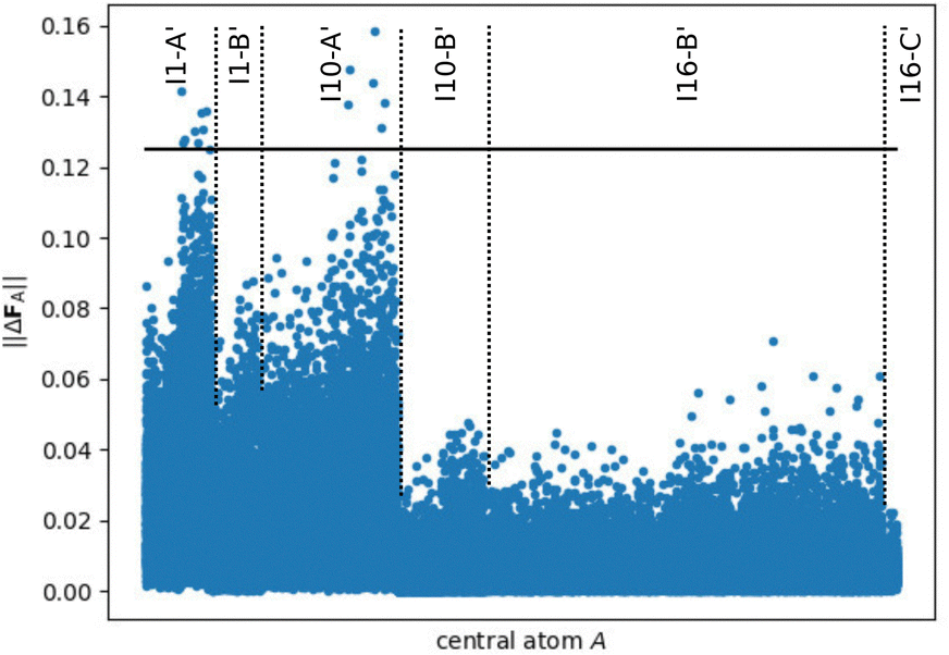 | ||
| Fig. 6 Norm of the DFT force errors ||ΔFA|| (in eV Å−1), i.e., the absolute difference between the force vectors in the periodic bulk structure and in the large fragments (Rconvfrag = 8.718 Å, cf.Fig. 5), for all central atoms in a bulk-like environment. The target accuracy for converged forces ||ΔFmax|| = 0.125 eV Å−1 (cf. ref. 48) is highlighted by the black line showing that the vast majority of atomic forces in the fragments is very similar to the periodic bulk system. | ||
The situation is different for the small fragments compiled in Fig. 7, which show clearly larger force errors. In particular a large number of I1-As fragments show prominent deviations up to about 0.35 eV Å−1. Therefore, it is evident that the small fragments do not provide bulk-like forces in DFT calculations and thus these forces could not be learned directly by HDNNP1, but can only be predicted based on the atomic energies.
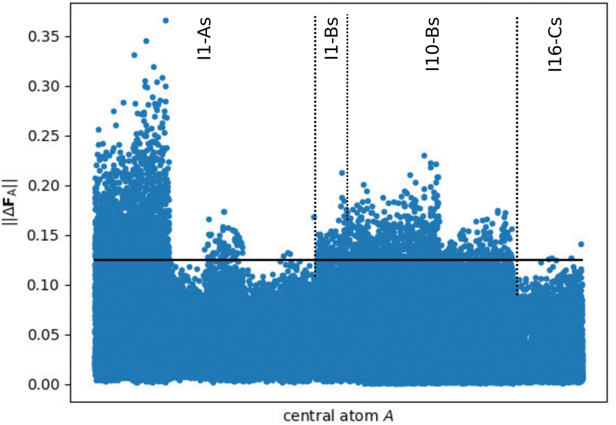 | ||
| Fig. 7 Norm of the DFT force errors ||ΔFA|| (in eV Å−1), i.e., the absolute difference between the force vectors in the periodic bulk structure and in the small fragments (Rfrag = 4.359 Å, cf.Fig. 3), for all central atoms with a complete environment within Rc. The criterion for converged forces ||ΔFmax|| ≤ 0.125 eV Å (conf. ref. 48) is highlighted by the black line showing that a significant part of the atomic forces in the fragments is substantially different from the periodic bulk system. | ||
Now we compute the energy and force RMSEs with respect to DFT of the 502 bulk validation structures for each MOF system using HDNNP1, HDNNP2, and HDNNP3. Again, a correction for the energy offset has been determined using the energy of the DFT optimized IRMOF bulk structures and the respective HDNNP predictions. The results are compiled in Table 6. All HDNNPs predict the bulk energies and atomic forces with excellent accuracy, with the largest force RMSE of 0.15 eV Å−1 found for IRMOF-16 predicted by HDNNP3, which is the most challenging case due to the large atomic environments to be sampled and the smallest number of training fragments for this MOF in the reference data set. Overall, the energy and force errors are at least comparable and in most cases even clearly below the errors of the respective fragments in the training and test sets in Tables 3 and 4. Most importantly, HDNNP1 provides the smallest force errors of all HDNNPs demonstrating that indeed the PESs of the periodic bulk MOFs can be learned from small, underconverged molecular fragments without making use of numerically bulk-like forces.
| HDNNP1 | HDNNP2 | HDNNP3 | |||||
|---|---|---|---|---|---|---|---|
| Validation set | Data points | RMSE | RMSE | RMSE | |||
| E | F | E | F | E | F | ||
| IRMOF-1 bulk | 502 | 0.0009 | 0.1041 | 0.0008 | 0.1100 | 0.0014 | 0.1301 |
| IRMOF-10 bulk | 502 | 0.0014 | 0.1174 | 0.0010 | 0.1312 | 0.0009 | 0.1513 |
| IRMOF-16 bulk | 502 | 0.0015 | 0.1149 | 0.0008 | 0.1319 | 0.0016 | 0.1501 |
4.5 Conclusion
In this work, we have shown for the example of high-dimensional neural network potentials that it is possible to train transferable second-generation MLPs yielding accurate forces for extended systems using only molecular fragments, which are too small to provide numerically converged bulk-like forces. The reason for this transferability from underconverged fragments to large systems is the analytic relation between the forces and the atomic energies, which have different formal interaction ranges with respect to the atomic environments. Since the forces can be derived as a sum of partial derivatives of the atomic energies, it is possible to predict accurate forces using the rather short-ranged environment-dependence of the atomic energies within the applied symmetry function cutoff only. A condition for this transferability of the forces is a rigorous determination of the system-specific physical interaction range, which can be determined from first principles for the case of the forces using the Hessian-based method reported in ref. 48. Then, half of this interaction range defines the minimum symmetry function cutoff of the atomic environments in the small fragments, which corresponds to the fragment radius that has to be applied in the construction of the reference data set.The absolute values of the fragment and cutoff radii depend on the system under investigation, and in the present work we have chosen the metal–organic-frameworks IRMOF-1, -10, and -16 for illustrating the feasibility of our approach. Moreover, the fragment radius depends on the desired level of accuracy of the forces. Following earlier work,48 for simplicity we have adopted a force convergence level of about 0.125 eV Å−1 here. Applying a more rigorous convergence criterion is possible, which then results in larger reference systems but does not affect the general finding of our work in that smaller fragments of half the size are still sufficient for obtaining transferable potentials. Using such fragments of decreased size enables to drastically reduce the costs of the electronic structure reference calculations employed in the construction of MLPs.
Beyond these general considerations, we have shown that for the explicit example of a series of MOFs the generation of potentials with transferable forces is indeed possible. For this purpose, three different HDNNPs have been developed employing (1) small fragments and a small cutoff, (2) large fragments and a small cutoff, and (3) large fragments and a large cutoff. For all these potentials a similar accuracy for the energies and forces in independent validation sets consisting of large fragments and periodic bulk structures have been found, confirming the possibility to construct transferable potentials for real systems. Interestingly, overall the HDNNPs constructed using a small symmetry function cutoff even show a generally better accuracy, which might be a consequence of the increased structural complexity to be described in case of large cutoff spheres and the corresponding larger amount of information that has to be provided in the reference data set. Our results are general and applicable to all types of second-generation MLPs.
Conflicts of interest
There are no conflicts of interest to declare.Acknowledgements
We thank the Deutsche Forschungsgemeinschaft (DFG) for financial support (BE3264/12-1, project number 405479457 as part of PAK 965/1). We gratefully acknowledge computing time provided by the DFG project INST186/1294-1 FUGG (Project No. 405832858).Notes and references
- J. Behler, J. Chem. Phys., 2016, 145, 170901 CrossRef PubMed.
- V. L. Deringer, M. A. Caro and G. Csányi, Adv. Mater., 2019, 31, 1902765 CrossRef CAS PubMed.
- P. O. Dral, J. Phys. Chem. Lett., 2020, 11, 2336–2347 CrossRef CAS PubMed.
- F. Noé, A. Tkatchenko, K.-R. Müller and C. Clementi, Annu. Rev. Phys. Chem., 2020, 71, 361–390 CrossRef PubMed.
- J. Behler and G. Csányi, Eur. Phys. J. B, 2021, 94, 142 CrossRef CAS.
- O. T. Unke, S. Chmiela, H. E. Sauceda, M. Gastegger, I. Poltavsky, K. T. Schütt, A. Tkatchenko and K.-R. Müller, Chem. Rev., 2021, 121, 10142–10186 CrossRef CAS PubMed.
- E. Kocer, T. W. Ko and J. Behler, Annu. Rev. Phys. Chem., 2022, 73, 163–186 CrossRef PubMed.
- T. W. Ko, J. A. Finkler, S. Goedecker and J. Behler, Acc. Chem. Res., 2021, 54, 808–817 CrossRef CAS PubMed.
- J. Behler, Chem. Rev., 2021, 121, 10037–10072 CrossRef CAS PubMed.
- J. Behler and M. Parrinello, Phys. Rev. Lett., 2007, 98, 146401 CrossRef PubMed.
- J. Behler, Angew. Chem., Int. Ed., 2017, 56, 12828 CrossRef CAS PubMed.
- S. Houlding, S. Y. Liem and P. L. A. Popelier, Int. J. Quantum Chem., 2007, 107, 2817–2827 CrossRef CAS.
- N. Artrith, T. Morawietz and J. Behler, Phys. Rev. B: Condens. Matter Mater. Phys., 2011, 83, 153101 CrossRef.
- K. Yao, J. E. Herr, D. W. Toth, R. Mckintyre and J. Parkhill, Chem. Sci., 2018, 9, 2261–2269 RSC.
- O. T. Unke and M. Meuwly, J. Chem. Theory Comput., 2019, 15, 3678–3693 CrossRef CAS PubMed.
- T. Bereau, D. Andrienko and O. A. von Lilienfeld, J. Chem. Theory Comput., 2015, 11, 3225–3233 CrossRef CAS PubMed.
- S. A. Ghasemi, A. Hofstetter, S. Saha and S. Goedecker, Phys. Rev. B: Condens. Matter Mater. Phys., 2015, 92, 045131 CrossRef.
- X. Xie, K. A. Persson and D. W. Small, J. Chem. Theory Comput., 2020, 16, 4256–4270 CrossRef CAS PubMed.
- T. W. Ko, J. A. Finkler, S. Goedecker and J. Behler, Nat. Commun., 2021, 12, 398 CrossRef CAS PubMed.
- K. T. Schütt, H. E. Sauceda, P.-J. Kindermans, A. Tkatchenko and K.-R. Müller, J. Chem. Phys., 2018, 148, 241722 CrossRef PubMed.
- J. S. Smith, O. Isayev and A. E. Roitberg, Chem. Sci., 2017, 8, 3192–3203 RSC.
- R. Zubatyuk, J. S. Smith, J. Leszczynski and O. Isayev, Sci. Adv., 2019, 5, eaav6490 CrossRef CAS PubMed.
- A. P. Bartók, M. C. Payne, R. Kondor and G. Csányi, Phys. Rev. Lett., 2010, 104, 136403 CrossRef PubMed.
- A. P. Bartók and G. Csányi, Int. J. Quantum Chem., 2015, 115, 1051–1057 CrossRef.
- A. V. Shapeev, Multiscale Model. Simul., 2016, 14, 1153–1173 CrossRef.
- A. P. Thompson, L. P. Swiler, C. R. Trott, S. M. Foiles and G. J. Tucker, J. Comput. Phys., 2015, 285, 316–330 CrossRef CAS.
- R. Drautz, Phys. Rev. B, 2019, 99, 014104 CrossRef CAS.
- R. M. Balabin and E. I. Lomakina, Phys. Chem. Chem. Phys., 2011, 13, 11710–11718 RSC.
- M. Rupp, A. Tkatchenko, K.-R. Müller and O. A. von Lilienfeld, Phys. Rev. Lett., 2012, 108, 058301 CrossRef PubMed.
- N. Artrith and J. Behler, Phys. Rev. B: Condens. Matter Mater. Phys., 2012, 85, 045439 CrossRef.
- J. Weinreich, A. Römer, M. L. Paleico and J. Behler, J. Phys. Chem. C, 2020, 124, 12682–12695 CrossRef CAS.
- M. Gastegger, C. Kauffmann, J. Behler and P. Marquetand, J. Chem. Phys., 2016, 144, 194110 CrossRef PubMed.
- M. Eckhoff and J. Behler, J. Chem. Theory Comput., 2019, 15, 3793–3809 CrossRef CAS PubMed.
- B. Huang and O. A. von Lilienfeld, Nat. Chem., 2020, 12, 945–951 CrossRef CAS PubMed.
- V. Zaverkin, D. Holzmüller, R. Schuldt and J. Kästner, J. Chem. Phys., 2022, 156, 114103 CrossRef CAS PubMed.
- J. Daru, H. Forbert, J. Behler and D. Marx, Phys. Rev. Lett., 2022, 129, 226001 CrossRef CAS PubMed.
- H. S. Seung, M. Opper and H. Sompolinsky, Proceedings of the fifth annual workshop on computational learning theory, 1992, pp. 287–294.
- J. S. Smith, B. Nebgen, N. Lubbers, O. Isayev and A. E. Roitberg, J. Chem. Phys., 2018, 148, 241733 CrossRef PubMed.
- E. V. Podryabinkin and A. V. Shapeev, Comput. Mater. Sci., 2017, 140, 171–180 CrossRef CAS.
- C. Schran, F. L. Thiemann, P. Rowe, E. A. Müller, O. Marsalek and A. Michaelides, Proc. Natl. Acad. Sci. U. S. A., 2021, 118, e2110077118 CrossRef CAS PubMed.
- J. Vandermause, S. B. Torrisi, S. Batzner, Y. Xie, L. Sun, A. M. Kolpak and B. Kozinsky, npj Comput. Mater., 2020, 6, 20 CrossRef.
- Z. Li, J. R. Kermode and A. D. Vita, Phys. Rev. Lett., 2015, 114, 096405 CrossRef PubMed.
- R. Jinnouchi, F. Karsai and G. Kresse, Phys. Rev. B, 2019, 100, 014105 CrossRef CAS.
- J. B. Witkoskie and D. J. Doren, J. Chem. Theory Comput., 2005, 1, 14–23 CrossRef CAS PubMed.
- A. Pukrittayakamee, M. Malshe, M. Hagan, L. M. Raff, R. Narulkar, S. Bukkapatnum and R. Komanduri, J. Chem. Phys., 2009, 130, 134101 CrossRef CAS PubMed.
- H. E. Sauceda, S. Chmiela, I. Poltavsky, K.-R. Müller and A. Tkatchenko, J. Chem. Phys., 2019, 150, 114102 CrossRef PubMed.
- V. L. Deringer and G. Csányi, Phys. Rev. B, 2017, 95, 094203 CrossRef.
- M. Herbold and J. Behler, J. Chem. Phys., 2022, 156, 114106 CrossRef CAS PubMed.
- M. Eddaoudi, J. Kim, N. Rosi, D. Vodak, J. Wachter, M. O'Keeffe and O. M. Yaghi, Science, 2002, 295, 469–472 CrossRef CAS PubMed.
- H. Furukawa, K. E. Cordova, M. O'Keeffe and O. M. Yaghi, Science, 2013, 341, 1230444 CrossRef PubMed.
- M. Li, D. Li, M. O'Keeffe and O. M. Yaghi, Chem. Rev., 2014, 114, 1343–1370 CrossRef CAS PubMed.
- M. Eddaoudi, D. B. Moler, H. Li, B. Chen, T. M. Reineke, M. O'Keeffe and O. M. Yaghi, Acc. Chem. Res., 2001, 34, 319–330 CrossRef CAS PubMed.
- D. J. Tranchemontagne, J. L. Mendoza-Cortés, M. O'Keeffe and O. M. Yaghi, Chem. Soc. Rev., 2009, 38, 1257–1283 RSC.
- Z. Wang and S. M. Cohen, Chem. Soc. Rev., 2009, 38, 1315–1329 RSC.
- M. Kalaj and S. M. Cohen, ACS Cent. Sci., 2020, 6, 1046–1057 CrossRef CAS PubMed.
- B. Li, M. Chrzanowski, Y. Zhang and S. Ma, Coord. Chem. Rev., 2016, 307, 106–129 CrossRef CAS.
- P. Horcajada, R. Gref, T. Baati, P. K. Allan, G. Maurin, P. Couvreur, G. Férey, R. E. Morris and C. Serre, Chem. Rev., 2012, 112, 1232–1268 CrossRef CAS PubMed.
- R. J. Kuppler, D. J. Timmons, Q.-R. Fang, J.-R. Li, T. A. Makal, M. D. Young, D. Yuan, D. Zhao, W. Zhuang and H.-C. Zhou, Coord. Chem. Rev., 2009, 253, 3042–3066 CrossRef CAS.
- L. Wang, Y. Han, X. Feng, J. Zhou, P. Qi and B. Wang, Coord. Chem. Rev., 2016, 307, 361–381 CrossRef CAS.
- F.-X. Coudert and A. H. Fuchs, Coord. Chem. Rev., 2016, 307, 211–236 CrossRef CAS.
- S. Chong, S. Lee, B. Kim and J. Kim, Coord. Chem. Rev., 2020, 423, 213487 CrossRef CAS.
- K. M. Jablonka, D. Ongari, S. M. Moosavi and B. Smit, Chem. Rev., 2020, 120, 8066–8129 CrossRef CAS PubMed.
- S. Vandenhaute, M. Cools-Ceuppens, S. DeKeyser, T. Verstraelen and V. V. Speybroeck, ChemRxiv, 2022, preprint DOI:10.26434/chemrxiv-2022-n1g60.
- O. Tayfuroglu, A. Kocak and Y. Zorlu, Phys. Chem. Chem. Phys., 2022, 24, 11882 RSC.
- J. Behler, J. Chem. Phys., 2011, 134, 074106 CrossRef PubMed.
- J. Behler, Int. J. Quantum Chem., 2015, 115, 1032–1050 CrossRef CAS.
- J. Behler, J. Phys.: Condens. Matter, 2014, 26, 183001 CrossRef CAS PubMed.
- V. Blum, R. Gehrke, F. Hanke, P. Havu, V. Havu, X. Ren, K. Reuter and M. Scheffler, Comput. Phys. Commun., 2009, 180, 2175–2196 CrossRef CAS.
- B. Hammer, L. B. Hansen and J. K. Nørskov, Phys. Rev. B: Condens. Matter Mater. Phys., 1999, 59, 7413–7421 CrossRef.
- A. Tkatchenko and M. Scheffler, Phys. Rev. Lett., 2009, 102, 073005 CrossRef PubMed.
- J. Nocedal and S. J. Wright, Numerical Optimization, Springer, New York, NY, 2006 Search PubMed.
- T. B. Blank and S. D. Brown, J. Chemometrics, 1994, 8, 391–407 CrossRef CAS.
- M. Eckhoff and J. Behler, npj Comput. Mater., 2021, 7, 170 CrossRef.
- M. Eckhoff and J. Behler, J. Chem. Theory Comput., 2019, 15, 3793–3809 CrossRef CAS PubMed.
- A. Singraber, J. Behler and C. Dellago, J. Chem. Theory Comput., 2019, 15, 1827–1840 CrossRef CAS PubMed.
- S. Plimpton, J. Comput. Phys., 1995, 117, 1 CrossRef CAS.
Footnote |
| † Electronic supplementary information (ESI) available. See DOI: https://doi.org/10.1039/d2cp05976b |
| This journal is © the Owner Societies 2023 |