
 Open Access Article
 This Open Access Article is licensed under a
 Creative Commons Attribution 3.0 Unported Licence
Disentangling the resonant Auger spectra of ozone: overlapping core-hole states and core-excited state dynamics†
Bruno Nunes Cabral
Tenorio
 *a,
Klaus B.
Møller
a,
Piero
Decleva
b and
Sonia
Coriani
*a
*a,
Klaus B.
Møller
a,
Piero
Decleva
b and
Sonia
Coriani
*a
aDepartment of Chemistry, Technical University of Denmark, Kemitorvet Bldg 207, DK-2800, Kongens Lyngby, Denmark. E-mail: brncat@dtu.dk; soco@kemi.dtu.dk
bIstituto Officina dei Materiali IOM-CNR and Dipartimento di Scienze Chimiche e Farmaceutiche, Università degli Studi di Trieste, I-34121 Trieste, Italy
First published on 7th November 2022
Abstract
We investigate the resonant and non-resonant Auger spectra of ozone with a newly implemented multi-reference protocol based on the one-center approximation [Tenorio et al., J. Chem. Theory Comput. 2022, 18, 4387–4407]. The results of our calculations are compared to existing experimental data, where we elucidate the resonant Auger spectrum measured at 530.8 and 536.7 eV, that correspond to the 1sOT → π*(2b1) and 1sOT → σ*(7a1) resonances, and at 542.3 eV, which lies near the 1sOC → σ*(7a1) excited state and above the 1sOT−1 ionization threshold. Using molecular dynamics simulations, we demonstrate the relevance of few-femtoseconds nuclear dynamics in the resonant Auger spectrum of ozone following the 1sOT → π*(2b1) core-excitation.
1 Introduction
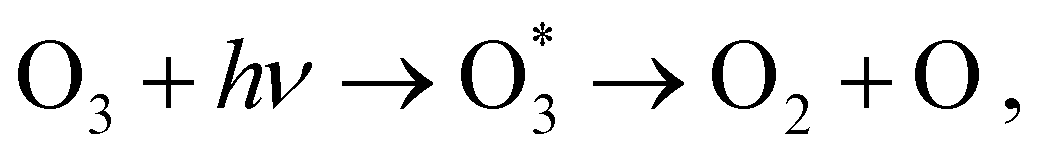
Ozone is a highly reactive homonuclear triatomic molecule oriented with C2v point group symmetry. The two molecular sites are denoted OC for the central oxygen atom, and OT for the terminal ones.1,2 Besides its fundamental relevance in Earth's atmosphere, ozone has also vast industrial and medicinal applications.3–6 Due to its relevance, the electronic spectroscopy of ozone has been extensively studied both at the valence7–11 and core-excited12–19 regions. Deep ultraviolet photodissociation of ozone following an excitation from the ground electronic state to the excited B(1B2) state [Hartley state], according tois responsible for the protective function of the ozone layer in the stratosphere, although the fourth ionized state of O3+ was also found to lead to photofragmentation of O3+ → O2 + O+ by visible light.2 Recently, the photodynamics of ozone leading to fast photofragmentation has been investigated using time-resolved photoelectron spectroscopy (PES) experiments.20,21
Molecular Auger electron spectroscopy22,23 (also known as Auger–Meitner24) is a very attractive experimental tool that encodes the electronic structure of a core-excited or core-ionized molecule into the kinetic energy of the ejected Auger electron mapping bound states to the continuum, and, essentially, probing molecular relaxation mechanisms. Processes involved in resonant Auger electron spectroscopy (RAES) are the ones that occur when a core-excited state decays to a singly ionized state, where the outgoing electron can be either the core-excited electron, resulting in a one-hole (1h) final state (participator Auger), or an inner-valence electron, resulting in a two-hole-one-particle (2h1p) state (spectator Auger). In normal (or non-resonant) Auger electron spectroscopy (AES), a core-ionized 1h initial state decays into a manifold of doubly charged (2h) valence states of different spin multiplicity. In the past few years, Auger spectroscopy has been extensively used in connection to X-ray absorption spectroscopy (XAS) and/or X-ray photoelectron spectroscopy (XPS) to probe site-specificity in molecular photofragmentation.25–29 Because of their high sensitivity to electronic and nuclear dynamics, AES/RAES are becoming increasingly popular techniques to unravel underlying electronic structure,30 and nuclear dynamics of photoexcited molecules.31–35
RAES measurements of ozone have been obtained with photon energies of 530.8 and 536.7 eV, which correspond to the 1sOT → π*(2b1) and 1sOT → σ*(7a1) excitations,12,13 and at 542.3 eV, that lies near the 1sOC → σ*(7a1) excited state and above the 1sOT−1 ionization threshold.13 For the case of the resonant 1sOT → σ*(7a1) state, a Doppler-type energy-split in the kinetic energy of atomic Auger electrons arising after fast fragmentation has been reported.13,36 The promotion of a core-electron into a repulsive intermediate electronic state can lead to fragmentation on a time scale compatible with a core-hole lifetime—that is, a few femtoseconds (fs).37 Ultrafast dissociation has been demonstrated to be an important mechanism of distributing the internal energy in core-excited small molecules like H2O,38 NH3,39 HCl40–42 as well as in heavier ones, such as CH2Cl2 and CHCl3.43–45
On the theory side, one of the main challenges in devising approaches to simulate Auger spectra is how to properly account for the contributions due to the electronic continuum wave function, whose asymptotic behavior is poorly described within the quadratically integrable finite (L2) basis sets typically employed for bound states. Notice, however, that total decay widths have been obtained with purely L2 basis sets and a Stieltjes imaging procedure,46 or by use of complex scaling of the Hamiltonian.47 Some attempts to bypass – or simplify – the problem of the electronic continuum in the context of Auger electron spectroscopy are methodologies based on simple population analysis of the final cationic states,48 or on the use of precalculated atomic bound-continuum two-electron integrals within the one-center approximation (OCA).49–52 Other computational strategies relying on explicit evaluation of the bound-continuum Auger intensities have been reported based on different flavours of electronic structure approximations for the bound and the continuum states.53–59 A second important issue is how to achieve a reasonably accurate description of the manifold of final states, and the relaxation associated with the core hole state. Resonant Auger typically explores a very large manifold of valence singly ionized states, covering some tens of eV, and spanning the inner valence part of the spectrum, so that, in addition to primary holes, mostly 2h1p states, and the large correlation effects associated with them become involved. Some methods may show a progressive drift of final states towards higher energies, due to insufficient correlation of the physical 2h1p states.57,58 Moreover, in propagator or linear response approaches employing a single set of orbitals, usually of the ground state, an accurate description of the core hole state, and its matrix elements with the final states, is also an additional problem, which calls for higher excitation levels. This is circumvented in configuration interaction (CI) approaches, which can employ separate orbital bases for the initial and final states. In this respect, O3 is a particularly challenging case, as already its ground state is highly correlated, and configuration mixing is dramatic in the ionic states, even at the start of the spectrum. Similar considerations apply to the normal Auger, where already the density of final primary 2h states is much higher, and 3h2p will be likely to be significantly excited, although this has not yet been investigated in so much detail.
Here we use the OCA to evaluate Auger decay rates based on a restricted-active-space perturbation theory of second order (RASPT2) description of the bound states. We recently implemented this OCA-RASPT2 approach52 within the OpenMolcas program.60 More specifically, we here demonstrate the capabilities of OCA-RASPT2 on the resonant and non-resonant Auger spectra of ozone, especially in a situation of overlapping core-hole states, as observed for the 1sOC → σ*(7a1) and 1sOT−1 states. Moreover, we demonstrate the relevance of few femtoseconds nuclear dynamics in the resonant Auger spectrum following the 1sOT → π*(2b1) core-excitation.
The paper is organized as follows: in Section 2, we give a brief description of the underlying theory of molecular Auger decay rates based on the Wentzel ansatz.61,62 In Section 3, the information about our computational protocol, and the molecular dynamics simulations is detailed. The results are presented and discussed in Section 4. Outlook and conclusions are given in Section 5.
2 Theory
Auger decay rates are here obtained from the Fermi golden rule61,62 (a.k.a. Wentzel's Ansatz) for the rate of decay of an isolated resonance interacting with a continuum, i.e., the transition| ΨNI → ΨN−1K + e−, | (1) |
In the Wentzel approximation,62,63 the core-excitation or core-ionization process that prepares the initial state is uncoupled from the subsequent decay processes, i.e., initial core-excitation/ionization and subsequent decay are treated as two independent steps. Only the decay process is explicitly considered.
For fixed initial (I) and final (K) states, the partial decay rate ΓKI (also known as Auger intensity or decay width) is obtained by a sum over all possible angular momenta of the Auger electron
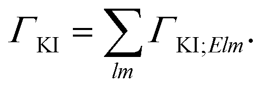 | (2) |
| ΓKI;Elm = 2π|〈ΨK;Elm|Ĥ − EI|ΨI〉|2. | (3) |
Here ΨK;Elm is the total N-electron final state wave function, which is approximated as an antisymmetrized product of a final (N − 1)-electron state wavefunction ΨN−1K and a continuum orbital ϕElm with kinetic energy E and angular momentum quantum numbers l and m,
| ΨK;Elm = ϕElmΨN−1K. | (4) |
| ΓKI;Elm = 2π|AKI;Elm + BKI;Elm|2, | (5) |
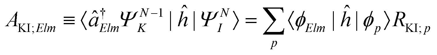 | (6) |
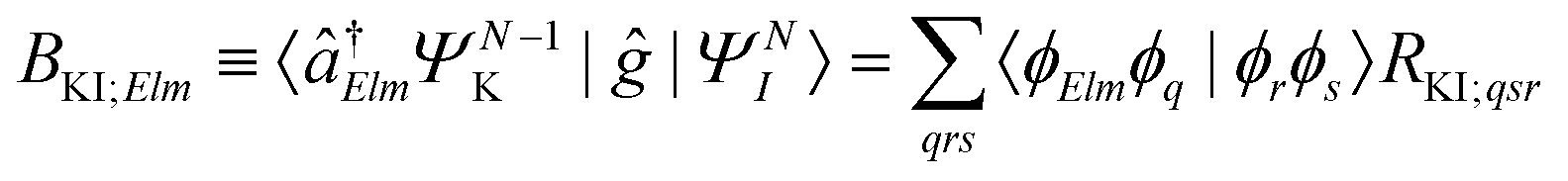 | (7) |
The matrix elements RKI;p in eqn (6) are the expansion coefficients of the one-particle Dyson orbital over the spin–orbital MO basis {ϕ},64,65
| RKI;p = 〈ΨN−1K|âp|ΨNI〉. | (8) |
The spin-adapted Auger matrix elements RKI;qsr (also called two-particle Dyson matrix) in eqn (7) can be expressed as (see, e.g., ref. 52, 55 and 66)
| RKI;qsr = 〈ΨN−1K|â†qâsâr|ΨNI〉 | (9) |
The remaining ingredients needed for the evaluation of the decay matrix element in eqn (5) are the one- and two-electron integrals involving the regular MO orbitals and the wave function of the continuum electron. As anticipated, we here use the technique called one-center approximation,49,50 which utilizes precalculated bound-continuum atomic two-electron integrals, and thereby avoids the explicit evaluation of the continuum wave function. OCA is based on the recognition of the strongly localized nature of the initial core hole, and it amounts to the neglect of coulomb matrix elements involving atomic orbitals (AOs) on different centers. Moreover, the continuum, expanded in partial waves centered on the core site, is approximated by the corresponding atomic one. Because of the high electron kinetic energy it is again a fair approximation. Due to the complexity and sheer number of final ionic states reached, OCA seems pretty adequate for an overall description of the spectral intensities in current spectra of complex molecules, unless an accurate study of specific, well-characterized, spectral features is warranted. A full description of the molecular continuum may be included, at a considerable computational cost, using for example a multicenter Bspline description of the continuum.67
Moreover, the one-center approximation49,50 considers the amplitude based on the Wentzel ansatz, eqn (5), where the matrix element ΓKI;Elm is reduced to the direct two-electron term (eqn (7)), as AKI;Elm is generally very small compared to BKI;Elm (see, e.g., ref. 52 and the investigation in ref. 56)
| ΓKI;Elm ≃ 2π|BKI;Elm|2. | (10) |
 | (11) |
Various recipes, largely equivalent, can be employed to obtain the coefficients Dνr from the molecular orbitals {ϕr}, typically by projecting {ϕr} onto the space spanned by a minimal basis set (MBS).50 The most practical choice, which we adopt here, is to use, as MBS, the first fully contracted functions of the atomic Gaussian Type orbital (GTO) basis, which are accurate representations of the atomic orbitals.52 For further details about our OCA-RASPT2 implementation and the selection of a MBS, please consult Tenorio et al.52
3 Computational details
Calculations of resonant and non-resonant Auger spectra, as well as of PES, XPS and XAS, have been performed at the multi-state RASPT2 (MS-RASPT2) level71–74 using the OpenMolcas program package.60 Auger transition rates were obtained according to the one-center approximation.52 PES and XPS spectra have been obtained from the squared norm of the Dyson orbitals representing the ionization channels (see, e.g., ref. 65 for details). The OCA-RASPT2 Auger intensities52 were obtained with a developer version of OpenMolcas.We adopted the cc-pVTZ basis set75 in all calculations. Multi-reference calculations of core-excited and core-ionized states28,76,77 relevant to, respectively, resonant and non-resonant Auger spectra were carried out by placing the relevant core orbitals in the RAS1 space and enforcing single electron occupation in RAS1 by means of the HEXS projection technique78 available in OpenMolcas,60 which corresponds to applying the core-valence separation technique.79 RAS2 was used for complete electron distribution, i.e., to define the complete active space. RAS3 was kept empty. An imaginary level shift of 0.25 Hartree was applied to avoid intruder state singularities in the MS-RASPT2 calculations. The employed active space is illustrated in Fig. 1. Three inner valence orbitals with O 2s character were kept out of the active space. Three 1sO orbitals were added to the RAS1 subspace, whereas twelve electrons are distributed over nine molecular orbitals in the RAS2 subspace. Final cationic states were obtained by state-averaging over several final states for each irreducible representation of the Cs point group symmetry.
 | ||
| Fig. 1 Molecular active orbitals of O3 from a Hartree–Fock calculation with C2v point group symmetry. The core orbitals (RAS1 subspace) have been localized. The HF binding energies of the valence occupied orbitals are shown with the corresponding MO. | ||
At its ground state the ozone molecule belongs to the C2v point group symmetry with experimentally determined structural parameters80 of rO–O = 1.28 Å, ∠ = 116.8°. The two different atomic sites are denoted OT for the pair of terminal oxygen atoms and OC for the central oxygen atom. Similar to what we did in previous studies,52,66 to facilitate the application and analysis of the OCA projection on symmetry equivalent atomic sites, we have reduced the point group symmetry from C2v to Cs, and localized the core orbitals by applying a Cholesky localization procedure.81 Moreover, we find it particularly convenient to use Cs symmetry because we calculate Auger spectra along a (dissociative) molecular dynamics trajectory, where Cs symmetry can always be applied. Auger transitions involving the pair of terminal oxygen atoms are obtained by summing the contributions of each localized OT site. The localized 1s orbitals are visualized in Fig. 1. Notice that the valence orbitals are not affected by the localization procedure.
Additionally, RASSCF adiabatic molecular dynamic simulations of core-excited states of ozone have been performed using the DYNAMIX program in OpenMolcas.60 The dynamics simulate 30 fs using step size of 0.242 fs for the 1sOT → π*(2b1) core-excited state. A Nosé–Hoover chain of thermostats was used to reproduce dynamics at a constant temperature of 300 K. Sixteen random initial conditions (geometries and momenta) were generated following a Maxwell–Boltzmann distribution at 300 K, based on a frequency calculation of the ground state.
A heuristic Lorentzian broadening of the discrete stick spectra (energies and transition rates) was used to simulate the spectra. The value of the full-width-at-half-maximum (fwhm) parameter used in all the Auger spectra was 0.30 eV, except for the average spectra. In the latter case, the average is obtained by broadening all discrete sticks together with fwhm of 0.20 eV, while the convoluted intensity is divided by the number of time steps considered in the interval. Since all theoretical methods employ approximations, they inherently include some error, which, however, can often be remedied by an overall shift to align with the energy axis of the experiment. Sources of error can be basis set limitation, or unaccounted correlation effects (most probably a combination of both), lack of relativistic effects. The rigid shift and other parameters used for plotting the XAS, XPS and PES are given in the corresponding figures.
All calculations were carried out on the DTU High-Performance Computer Cluster.82
4 Results and discussion
The electronic ground state of ozone has a pronounced biradical character. It mixes the HF configuration with another orbital configuration reached by double excitation from the 1a2 to the 2b1 orbital.83 The leading valence configurations and their squared amplitudes given by a CASSCF wave function are given below:| (5a1)2(3b2)2(1b1)2(4b2)2(6a1)2(1a2)2(2b1)0[0.77] + (5a1)2(3b2)2(1b1)2(4b2)2(6a1)2(1a2)0(2b1)2[0.11]. |
We start with the description of the PES, XAS and XPS spectra. Notice that the final states on a PES spectrum are singly-charged cationic states, and they are usually the same as the final states reached after a resonant Auger decay process. Therefore, besides an appropriate description of the (initial) core-excited state, it is extremely important to be able to reproduce well the entire PES in order to have a decent description of the RAES. The multi-configurational character of ozone poses additional challenges for highly correlated methods based on a single determinant reference because of the configuration interaction already in the ground state. In Fig. S1 (ESI†), we show the PES obtained at the EOM-CCSD/cc-pVTZ level with the experimental ground state geometry80rO–O = 1.28 Å, ∠ = 116.8° (calculations performed with Q-Chem84). From Fig. S1 (ESI†), we observe that except for the first two peaks below 14 eV, the remaining part of the spectrum, dominated by multi-electron excitations, is not well reproduced by the EOM-CCSD method. Further improvements on the PES spectrum of ozone could possibly be reached with an EOM-CC3 (or EOM-CCSDR(3)) description of the ground and ionized states, as it was recently shown by Moitra et al.85 A recent implementation of multireference algebraic diagrammatic construction theory (MR-ADC)86 has also demonstrated excellent performance on the XPS spectrum of ozone.
Here we profit from the characteristics of the MS-RASPT2 level of approximation, as a multi-reference method allowing for a full-CI description of the excitation manifold within an active space, with dynamical correlation recovered by perturbation theory of second order.
4.1 PES, XAS and XPS
Valence photoelectron spectra of ozone have been extensively investigated experimentally and theoretically over the past decade.8–12,20,21,87 Our results are presented in Fig. 2 alongside with the experimental data.12 The peaks labeled I to V are characterized in Table 1. Peaks I and II are the only direct photoionization channels—that is, they can be represented by the removal of one electron from an occupied orbital. A direct ionization is also referred to as a 1h configuration. These peaks were also captured in the EOM-CCSD spectrum of Fig. S1 (ESI†). Peaks III to V are mostly satellites, and they can be generally represented by 2h1p orbital configurations. The calculation of PES comprising direct and satellite ionization channels is a useful test to check whether the electronic structure method employed is well suited for the calculation of resonant Auger spectra, which are known to be dominated by 2h1p spectator decay channels. From the observed agreement of our PES with the experimental measurement,12 we conclude that our protocol, based on the RASPT2 description of the bound states, is appropriate for the representation of the relevant states involved in the resonant Auger spectra of ozone. | ||
| Fig. 2 PES of O3. The spectrum was shifted by +0.3 eV and broadened with Lorentzian functions with fwhm = 0.18 eV. For the assignments of the peaks, see Table 1. | ||
| Binding energy (eV) | PESa | RAESb | Ionization characterc | |||
|---|---|---|---|---|---|---|
| This work | Exp.12 | Peak | R I | Peak | Γ (× 10−4 a.u.) | |
| a See also Fig. 2. b See also Fig. 4. c The numbers within square brackets correspond to the CI weight of the given configuration. | ||||||
| 12.52 | 12.8 | I | 0.84 | A | 0.40 | 6a1−1[0.73] |
| 12.59 | 12.8 | I | 0.81 | A | 0.39 | 4b2−1[0.75] |
| 13.50 | 13.5 | II | 0.77 | B | 1.21 | 1a2−1[0.83] |
| 14.61 | 0.18 × 10⁻³ | C | 0.66 | 6a1−22b11[0.47] + 4b2−22b11[0.38] | ||
| 15.67 | 0.87 × 10⁻² | D | 1.41 | 6a1−11a2−12b11[0.83] | ||
| 15.81 | 0.46 × 10⁻² | D | 1.40 | 4b2−11a2−12b11[0.81] | ||
| 16.67 | ∼16.5 | III | 0.24 | E | 1.28 | 1a2−22b11[0.58] |
| 17.29 | 0.33 × 10⁻² | E' | 1.72 | 4b2−16a1−12b11[0.62] | ||
| 17.78 | ∼17.5 | IV | 0.18 | 0.40 | 4b2−11a2−12b11[0.44] + 6a1−22b11[0.19] | |
| 17.80 | IV | 0.12 | E′′ | 1.23 | 6a1−22b11[0.24] + 4b2−22b11[0.29] | |
| 19.07 | 0.11 × 10⁻³ | F | 0.40 | 6a1−21a1−12b12[0.37] + 4b2−21a1−12b12[0.38] | ||
| 20.05 | ∼20.0 | V | 0.39 | 0.12 | 5a1−1[0.29] + 6a1−27a11[0.15] | |
| 20.35 | V | 0.55 | 0.16 | 4b2−11b1−12b11[0.39] + 3b2−1[0.18] | ||
| 21.01 | V | 0.51 | G | 1.37 | 1b1−1[0.38] | |
| 21.61 | 0.26 | H | 0.77 | 3b2−1[0.43] | ||
| 24.16 | 0.79 × 10⁻² | I | 1.07 | 3b2−11a2−12b11[0.65] | ||
| 24.16 | 0.74 × 10⁻² | I | 1.07 | 4b2−16a1−11b1−1 2b12[0.25] | ||
Here, we give only a brief description of our results for the XAS and XPS spectra since the absorption and ionisation spectra of ozone near the O 1s edge are well documented elsewhere.13,15,16,19,86,89,90 The assignments of the main features of the XAS and XPS are given in Table 2. The intense peak calculated at 528.9 eV in the XAS spectrum is assigned to the 1sOT → π*(2b1) state. The next core-excited state, computed at 535.7 eV, corresponds to an excitation of an 1sOC electron to the same π*(2b1) orbital. Notice that the separation between these two core-excitations involving the π*(2b1) is around 6 eV. A similar energy separation is also observed in the XPS for the ionization channels 1sOT−1 and 1sOC−1, calculated at 541.5 and 547.3 eV, respectively. Our core-ionization energies are also in good agreement with other calculated results based on MR-ADC.86 The excitation energies for the 1sOT → σ*(7a1) and the 1sOC → σ*(7a1) states were calculated as 536.4 and 541.0 eV, respectively.
| Label | Energy (eV) | O.S. | Excitation character | ||
|---|---|---|---|---|---|
| This work | Exp.13 | Exp.19 | |||
| A | 528.95 | 529.4 | 529.25 | 0.074 | 1sOT → π*(2b1) |
| B | 535.75 | ∼535.0 | 534.80 | 0.031 | 1sOC → π*(2b1) |
| C | 536.41 | ∼536.7 | 535.75 | 0.067 | 1sOT → σ*(7a1) |
| D | 538.76 | ∼538.0 | 537.90 | 0.039 | 1sOT → σ*(5b2) |
| E | 541.05 | ∼542.3 | 539.70 | 0.031 | 1sOC → σ*(7a1) |
| F | 543.02 | 542.00 | 0.062 | 1sOC → σ*(5b2) | |
In the following we concentrate on the discussion of the resonant Auger spectra of O3 at the 1sOT → π*(2b1), 1sOT → σ*(7a1) and 1sOC → σ*(7a1) resonances. The red arrows drawn in Fig. 3 – placed at 530.8, 536.7 and 542.3 eV – point to the regions of the spectrum where Auger spectra have been measured.12,13 The first arrow indicates an energy matching with the 1sOT → π*(2b1) resonance. The second arrow shows the photon energy intentionally blue-shifted relative to the 1sOT → σ*(7a1) resonance to avoid overlap with the 1sOC → π*(2b1) state. The third arrow is found in a region of the spectrum where the 1sOC → σ*(7a1) resonance and the 1sOT−1 ionization are close. In our calculations, the 1sOC → σ*(7a1) and the 1sOT−1 states are separated by just 0.5 eV, and therefore, they can be both accessed in the same measurement with photon energy of 542.3 eV, which lies above the ionization threshold of the 1s electron of the terminal O.13
 | ||
| Fig. 3 XAS (left) and XPS (right) of O3. The computed XAS and XPS spectra were shifted by +0.15 and +0.25 eV, and broadened with Gaussian functions with fwhm = 0.45 and 0.65 eV, respectively. The dashed vertical line in the experimental XAS spectrum indicates the first O1s ionization potential. The XAS and XPS experimental spectra were digitized from ref. 13 and 88, respectively. For a characterization of the labeled peaks, see Table 2. The red arrows indicate the photon energies where RAES have been measured. | ||
4.2 Auger spectroscopy
The RAES at the 1sOT → π*(2b1) resonance of O3 is presented in Fig. 4. The assignments of the main features of the spectrum are given in Table 1. In the calculation we used the experimental equilibrium geometry of the ground state80 (rO–O = 1.28 Å, ∠ = 116.8°). The calculated spectrum was shifted by −0.6 eV to better compare with the experiment. | ||
| Fig. 4 RAES of O3 at the 1sOT → π*(2b1) resonance calculated with the FC geometry. The computed spectrum was shifted by −0.6 eV and broadened with Lorentzian functions with fwhm = 0.30 eV. The experimental spectrum was digitized from ref. 12. For the assignments, see Table 1. | ||
By comparing the calculated RAES spectrum of Fig. 4 with experiment,12 we observe a satisfactory match only in the initial part of the spectrum, that is, for the three weak peaks observed between 517–514 eV, labeled A, B and C. These peaks are assigned to the participator decay channels 6a1−1 (A), 4b2−1 (A), and 1a2−1 (B) calculated at 515.9, 515.9, 515.1 eV, respectively, and the spectator decay channel 6a1−22b11 + 4b2−22b11 (C), calculated at 514.2 eV. Notice that, in contrast to peaks A and B, peak C is a dark state in the PES.12 The wave function of the ionic state corresponding to peak C has multiconfigurational character 6a1−22b11 + 4b2−22b11 with similar squared amplitudes. Thus, the photoionization probability for such state will be naturally very low due to configuration mixing, while resonant excitation leads to intensity redistribution via excitation to the π*(2b1) orbital, enhancing the probability for such state in RAES.83 The most intense peak on the RAES is observed in the experimental spectrum at around 512 eV (ionic states E, E′, and E′′), and it is underestimated to a large extent in our calculation. Peaks E, E′, and E′′ are mainly attributed to the decay channels 1a2−22b11, 4b2−16a1−12b11, and 6a1−22b11 + 4b2−22b11 (see Table 1). The broad peaks observed in the experiment between 509 and 507 eV are shifted to lower energies by ∼2 eV in the calculated spectrum. These peaks have characteristics of spectator as well as participator decay channels involving the deep valence molecular orbitals 1b1, 3b2 and 5a1, as one can see from the assignments in Table 1.
Overall, except for the peaks A–C, the agreement between the calculated spectrum obtained in the Franck–Condon regime and the experiment is quite poor. We note that another computed RAES at the 1sOT → π*(2b1) resonance with characteristics very similar to the ones obtained here was reported in ref. 12, although it is unclear to us why the authors chose to use structural parameters (rO–O = 1.19 Å and ∠ = 117.4°) so different from the experimentally determined ground state equilibrium geometry80 (rO–O = 1.28 Å and ∠ = 116.8°) or any other calculated structural parameters obtained for ozone.83,91–94
Our computed total decay rate for the 1sOT → π*(2b1) resonance is Γ = 25.6 × 10⁻⁴ a.u. This value can be possibly underestimated as any contribution from decay channels below 500 eV is neglected in our calculation. Full diagonalization of the Hamiltonian matrix would be necessary for a better estimate of the total decay rate, which is beyond our reach. Therefore, our model provides a lower bound of the total decay rate. The decay rate is converted to lifetime by the taking the reciprocal of Γ, τ = 1/Γ ⋍ 9 fs. This value is higher than the approximate lifetime of the O1s core hole in water,95 that is, ∼4 fs, possibly a consequence of an underestimation of Γ in our calculation.
In the following we combine trajectory molecular dynamics with Auger spectral calculations to characterize the features observed on the RAES of ozone following the 1sOT → π*(2b1) resonance.
The trajectories were obtained in the adiabatic regime, thus neglecting autoionization and possible interference between different pathways. According to the analysis of the XAS, the separation between the first 1sOT → π*(2b1) and the second electronic core-excited state 1sOC → π*(2b1) amounts to 6 eV, and therefore the adiabatic condition is expected to be a good approximation for a short time regime. It is important to highlight that our major interest is in describing the influence of molecular dynamics following the 1sOT → π*(2b1) excitation on the Auger spectrum of O3, and, particularly, the dynamics in a time regime compatible to the core-hole lifetime. Ultrafast dissociation was experimentally demonstrated in ozone for the 1sOT → σ*(7a1) resonance,13 but it was not observed in the experimental RAES at the 1sOT → π*(2b1) resonance.12
The core-excited molecular dynamics of ozone leads to the O3→O2 + O fragmentation if we allow the dynamics to run long enough, above the core-hole lifetime. In Fig. S2 (ESI†) we plot, for both the 1sOT → π*(2b1) and the 1sOT → σ*(7a1) states, the bond distance rO–O of the leaving oxygen (relative to the central oxygen) against the dynamics time up to 30 fs. The slope of the curves can be interpreted as an estimate of the velocity of the leaving oxygen  . From the slopes of Fig. S2 (ESI†), we can see that the 1sOT → σ*(7a1) dynamics is clearly faster compared to the 1sOT → π*(2b1) dynamics. For example, at 8 fs, the 1sOT → σ*(7a1) dynamics shows rO–O ∼ 1.8 Å, whereas the 1sOT → π*(2b1) dynamics shows rO–O ∼ 1.5 Å. In Fig. 5, we show some snapshots along a selected trajectory where the fragmentation of O3 into O2 + O can be visualized up to 20 fs. A common behaviour shared by all trajectories is that when one O–O bond increases, the other O–O bond decreases to be ultimately stabilized around 1.20 Å, which is nearly the equilibrium bond length of the O2 molecule.
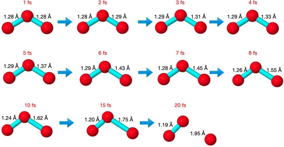 | ||
| Fig. 5 Snapshots along a selected trajectory of O3 at the 1sOT → π*(2b1) core-excited state. | ||
In Fig. 6, we show the molecular dynamics of the 1sOT → π*(2b1) state below 10 fs. A visual inspection shows that all the trajectories share similar characteristics, and therefore we will concentrate the analysis that follows only on the most central trajectory, that is the one represented by the dashed blue line.
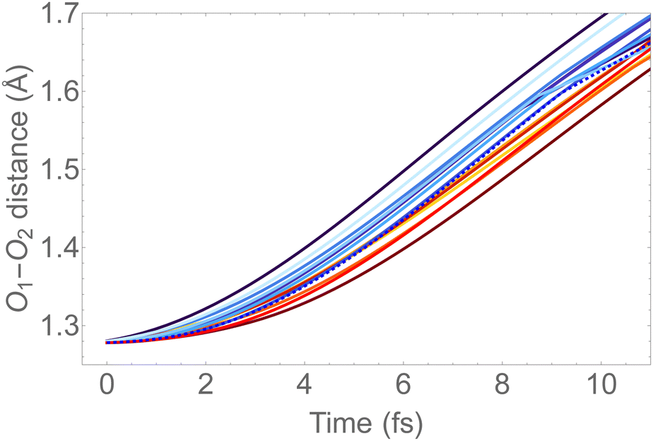 | ||
| Fig. 6 O–O bond length vs. time extracted from the trajectory molecular dynamics at the 1sOT → π*(2b1) core-excited state at the RASSCF level. We used sixteen initial conditions obtained from a Maxwell-Boltzmann distribution at 300 K (see Fig. S2 (ESI†) for the complete dynamics simulation up to 30 fs). | ||
The dynamics described by the trajectory shows almost zero velocity and practically no alteration on the bond length up to 2 fs. After 4 fs, the velocity (slope) becomes nearly constant. In the region between 4 and 8 fs, the bond lengths increase from ∼1.35 Å to ∼1.55 Å (see also Fig. 5).
For the sake of comparison, we can consider an approximately linear behaviour on the trajectories of Fig. S2 (ESI†) from 4 to 10 fs. Then, we estimate the average velocity  from our dynamics as ∼0.04 and 0.07 Å fs−1, for the 1sOT → π*(2b1) and 1sOT → σ*(7a1) resonances, respectively. The velocity of the leaving O atom relative to the O2 fragment, estimated from a classical mechanical model for the dissociation derived from the Doppler-split resonant Auger lines for the 1sOT → σ*(7a1) resonance, was reported as 0.0756 Å fs−1 in ref. 13. Comparing the approximate velocity of the 1sOT → π*(2b1) resonance with the one estimated with the classical mechanical model for the 1sOT → σ*(7a1) resonance,13 we find that our estimate is indeed in the same order of magnitude, but about 40% lower. This deviation was expected since we are comparing velocities from different excitation states, and we expect the relative velocity of the leaving oxygen obtained for the 1sOT → π*(2b1) resonance to be slower, since this state is less dissociative. On the other hand, the agreement between our molecular dynamics and the classical model13 concerning the relative velocity for the 1sOT → σ*(7a1) resonance is remarkable. These results suggest that the dynamics of the O3 at the few femtoseconds regime is described by our simulations quite decently.
To keep the time-resolved Auger spectra simulation computationally amenable, and to make sure that we are sampling the molecule within the core-hole lifetime, we simulate the first 9 fs along the most central trajectory represented by the dashed blue curve in Fig. 6, using a step size of 0.242 fs.
The time-resolved RAES spectra based on the most central trajectory is presented in details in Fig. 7. In the 3D plot (top panel of Fig. 7) we use a rainbow color code, in which the colors go from violet to red as the time increases. In the middle part of Fig. 7, the calculated spectra up to 4 fs are plotted in the left panel, and the spectra obtained from 4 to 9 fs are plotted in the right panel. Here, it is already possible to make a few comments. Before 4 fs, very little changes compared to the spectrum obtained with Franck–Condon geometry. Only above 4 fs, some meaningful changes in the spectra can be noticed. These observations are in agreement with our previous discussion of the structural parameters. The effect of the dynamics on the Auger spectra is revealed by the peak centered at around 512 eV which starts getting intensity at around 5 fs, and by the features between 505 and 509 eV, that decrease as time evolves. Using the snapshot corresponding to the molecular structure obtained at around 7 fs, we assign the intense peak near 512 eV to two spectator decay channels with the following orbital characteristics: 6a1−11a2−12b11 + 4b2−11a2−12b11 and 1a2−22b11, calculated at 512.56 and 512.70 eV, respectively. The spectrum and the effect of the distorted geometry on the involved molecular orbitals is shown in Fig. S3 (ESI†). At the distorted geometry, the electronic density of the valence molecular orbital 6a1 becomes similar to an O 2p orbital localized on the leaving oxygen. The electronic density of the virtual 2b1 orbital remains practically unaltered.
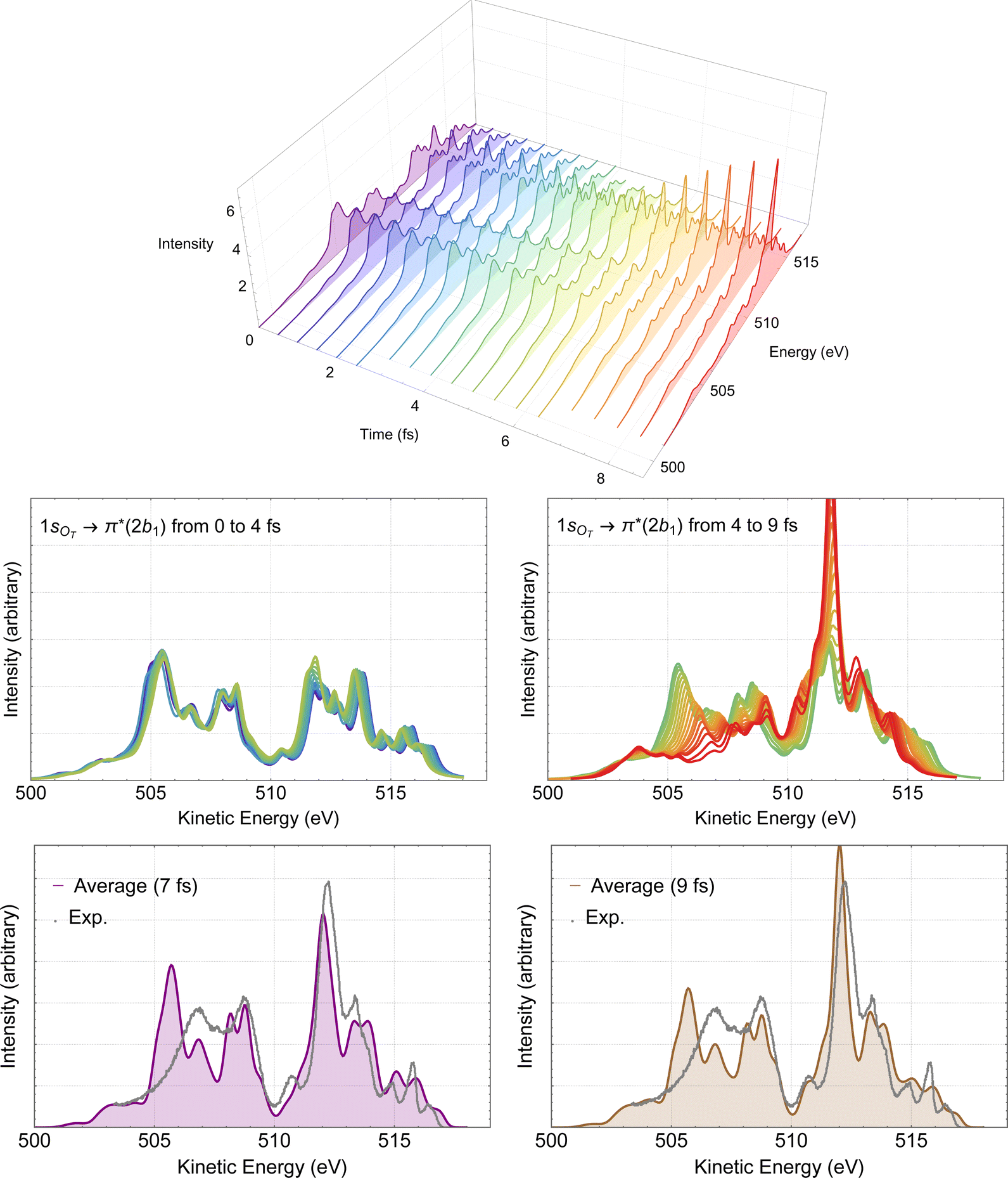 | ||
| Fig. 7 RAES of O3 at the 1sOT → π*(2b1) resonance. The selected trajectory along which the simulation is performed corresponds to the central trajectory represented by the dashed blue curve in Fig. 6. The computed spectra were shifted by –0.6 eV and broadened with Lorentzian functions with fwhm = 0.30 eV. In the top we show the 3D plot of the time-resolved spectra. In the middle, on the left we have the superposition of all spectra up to 4 fs, and on the right, from 4 to 9 fs. In the bottom, we consider the averaged (time integrated) spectra of the central trajectory up to 7 fs (left) and to 9 fs (right), plotted together with the experimental data digitized from ref. 12. | ||
The time-integrated spectrum (bottom panels of Fig. 7) is given by the average of all the calculated spectra along the selected trajectory. Here we consider two averages, one obtained integrating on the time up to 7 fs (left panel), and one up to 9 fs (right panel). We observe that both averages agree quite well with each other, as well as with the experiment. Overall, the agreement between these averaged spectra and experiment is much nicer than what we observed at the Frank–Condon geometry, see Fig. 4. Similar analysis based on different trajectories (not shown) yielded very similar characteristics as the ones presented in Fig. 7. Therefore, we suggest that the intense peak around 512 eV, as well as the features between 505 and 509 eV observed in the experimental spectrum are the result of ultrafast nuclear relaxation of ozone following the 1sOT → π*(2b1) resonance.
Notice that we ruled out ultrafast dissociation as the cause of the increase of the peak at 512 eV since there is no correspondence in the atomic oxygen Auger spectrum matching this energy,96 and the dynamics given in Fig. 6 have no indication of bond fragmentation below 10 fs.
In Fig. 8, the computed RAES following the 1sOT → σ*(7a1) resonance of ozone is presented together with the experimental spectrum.13 The calculation was performed at the ground state equilibrium geometry. The computed spectrum was shifted by +0.15 eV to better compare with experiment. The computed total decay rate was obtained as Γ = 28.1 × 10⁻⁴ a.u. As anticipated, the ozone molecule undergoes ultrafast dissociation at the 1sOT → σ*(7a1) resonance,13 which is characterized by the presence of atomic Auger lines together with the molecular Auger features. In Fig. 8, we used black bars to indicate the energies of the atomic oxygen Auger lines corresponding to the multiplets 4P(498.5 eV), 2P(508.4 eV) and 2D(510.1 eV), which values were obtained from ref. 96. The Auger spectrum calculated at the ground state equilibrium geometry shows a nice agreement with the experimental spectrum, except for the features corresponding to purely atomic decay. The first two peaks of the RAES are assigned to the participator Auger decays to the direct ionization channels 6a1−1(523.2 eV), 4b2−1(523.2 eV) and 1a2−1(522.3 eV). The strongest peak observed around 513 eV is assigned to a spectator decay state with mixed configuration [with squared amplitudes] 1a2−27a11[0.26] + 4b2−27a11[0.21] + 6a1−27a11[0.15]. Notice that the mixed configurations of the cationic state have in common a double hole in one upper valence orbital, and an excited electron in the σ*(7a1) orbital. In ref. 59, resonant Auger spectra of ozone following core-excitations from the OT and OC to a σ* orbital are reported from a CIS description of the bound states that incorporates post-collision effects by explicitly evaluating the continuum electronic wavefunction. Despite the poor electronic structure description of the bound states given by CIS, which prevents direct comparison with the experimental resonant Auger spectrum, our results are in fair agreement with the findings of the authors.59
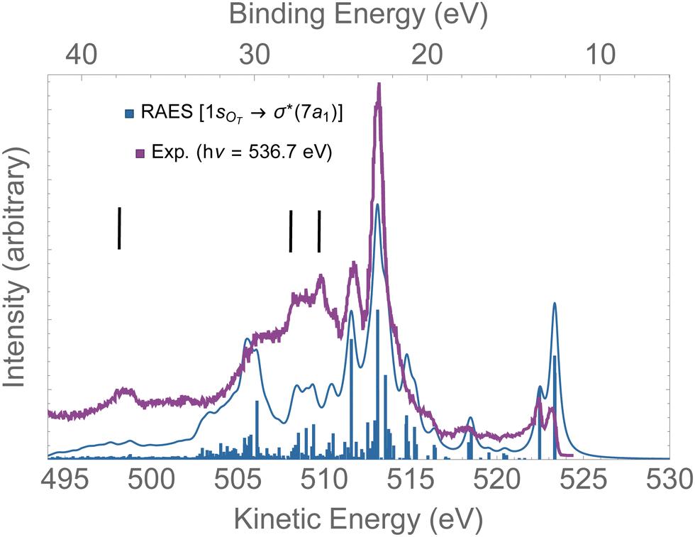 | ||
| Fig. 8 RAES of O3 at the 1sOT → σ*(7a1) resonance. The computed spectrum was shifted by +0.15 eV and broadened with Lorentzian functions with fwhm = 0.30 eV. The experimental data were digitized from ref. 13. The black bars indicate the energies of the atomic oxygen Auger decay. | ||
Overall, for the case of the 1sOT → σ*(7a1) resonant Auger decay, as the dynamics is significantly faster compared to the 1sOT → π*(2b1) state, we then suggest that most of the features exhibited by the experimental measurement13 resulted from resonant Auger decay of ozone either around the Franck–Condon structure, or when the molecule is already dissociated, yielding atomic Auger lines.
In Fig. 9, we investigate the experimental spectrum obtained with photon energy of 542.3 eV.13 As we already anticipated, at that energy one can access both the 1sOC → σ*(7a1) resonance and the 1sOT−1 ionization due to the small energy separation between these two states. In the top panel of Fig. 9, we have the resonant Auger spectrum computed for the 1sOC → σ*(7a1) resonance plotted together with the experimental spectrum.13 The calculated spectra (resonant and non-resonant) were shifted by +1.3 eV to better compare with the experiment. On the region comprising kinetic energies ranging from 530 to 510 eV, we observe a very good match with the experiment. The intense peak around 504 eV present in the experiment does not come from any contribution observed in the resonant Auger spectrum. However, from the normal Auger spectrum, shown in the middle panel of Fig. 9, we see the intense peak around 504 eV, and nothing in the region between 530 to 510 eV – which was otherwise rich in the resonant decay spectrum. If we now assume that both core-hole states can be accessed equally by the photon flux, we can thus plot the Auger spectrum stemming from the average of both the RAES (1sOC → σ*) and AES (1sOT−1). The average spectrum is presented in the bottom panel of Fig. 9. The intensity distribution of the average spectrum approximates quite well the relative intensities of the experimental spectrum, suggesting that our assumption of equal proportions of RAES (1sOC → σ*) and AES (1sOT−1) being obtained in the experimental spectrum recorded with photon energy of 542.3 eV13 is fairly reasonable.
 | ||
| Fig. 9 In the top panel, the RAES of O3 at the 1sOC → σ*(7a1) resonance is plotted alongside with the experimental spectrum.13 In the middle panel, the AES at the 1sOT−1 edge is shown. In the bottom panel, the sum of AES and RAES contributions are plotted. The computed spectra (RAES and AES) were shifted by +1.3 eV and broadened with Lorentzian functions with fwhm = 0.30 eV. The experimental data were digitized from ref. 13. | ||
5 Summary and conclusions
In the present study, we have given insights to and new interpretations of the experimental resonant Auger decay spectra of ozone measured at different regions of the XAS spectrum.12,13 Our study is based on a newly implemented RASPT2 one-center-approximation protocol52 and on molecular dynamics simulations. For the 1sOT → π*(2b1) resonant Auger spectrum, we have demonstrated the relevance of few femtosecond molecular dynamics, specially connected with a prominent feature observed at around 512 eV, emerging after 4 fs from the creation of the core-hole state. The average resonant Auger spectra that includes all snapshots along a selected central molecular dynamics trajectory up to either ∼7 or 9 fs (that is, compatible with the core-hole lifetime) demonstrate excellent agreement with the experimental spectrum measured with synchrotron light source.12Due to the much faster dynamics of the 1sOT → σ*(7a1) state, we observed that the resonant Auger spectrum obtained at the Franck-Condon geometry compares quite well with the experimental spectrum,13 except for a few atomic features. As a consequence of the dynamics of the 1sOT → σ*(7a1) state, the excited molecule initiates an ultrafast fragmentation process, resulting in the possibility of the Auger decay to take place either around the Franck–Condon region, or as dissociated fragments, yielding atomic Auger lines. Our argument agrees with the experimental observations that have demonstrated ultrafast dissociation following the 1sOT → σ*(7a1) state, but not for the 1sOT → π*(2b1) resonance. Additionally, to disentangle the experimental spectrum recorded with a photon energy of 542.3 eV,13 that lies above the core ionization threshold of the terminal oxygen, we evaluated the individual contributions stemming from the RAES (1sOC → σ*(7a1)) and AES (1sOT−1) spectra. Assuming that the photon flux can produce a 1sOC → σ*(7a1) excitation or a 1sOT−1 core-ionized state with equal probability, we plotted the average spectrum obtained from the RAES and AES together, which shows excellent agreement with the experimental measurement.13
Hence, we have obtained accurate Auger spectra based on a cost-effective computational protocol that, thanks to the one-center approximation, simplifies the electronic continuum problem.52 In situations where Auger experiments are recorded in a spectral region of overlapping core-hole states, the protocol presented here can give valuable insights to the interpretation of such experiments. Affordable computational protocols like ours are extremely useful for simulating time-resolved Auger spectra, e.g., based on molecular dynamics simulations. In future works, we also plan to incorporate the simulation of ultrashort pump pulses, as the ones used in modern pump–probe experiments,20 to capture manifestation of ultrafast chemistry in the Auger spectrum of excited molecules.
Within the OCA, post-collisional interaction effects and interference between the resonant Auger and direct channels are neglected, since the continuum wavefunction in the molecular environment is not calculated. Another possible limitation of the OCA concerns its ability to properly describe angular distributions. Despite previous work based on the OCA,97 one could argue that for an accurate description of angular distribution of the escaping electron, the shape of the continuum wavefunction within the scattering region must be explicitly evaluated. We are currently extending our method to utilize an explicit multicenter Bspline description of the continuum67 which will remedy these limitations. The Auger-Bspline approach is, of course, computationally more demanding compared to the cost-effective Auger-OCA method. Hence, the choice between using OCA or the explicit Bspline continuum will depend on the final application.
Conflicts of interest
There are no conflicts to declare.Acknowledgements
This work was carried out with support from the European Union's Horizon 2020 Research and Innovation Programme under the Marie Skłodowska-Curie Individual Fellowship (B.N.C.T., Grant Agreement 101027796), and from the Independent Research Fund Denmark – Natural Sciences, DFF-RP2 Grant No. 7014-00258B (S.C.). The European Cooperation in Science and Technology, COST Action CA18222, Attochem, is also acknowledged.Notes and references
- B. J. Finlayson-Pitts and J. N. Pitts, Chemistry of the Upper and Lower Atmosphere: Theory, Experiments, and Applications, Academic Press, San Diego, 2000 Search PubMed.
- S. P. Goss and J. D. Morrison, J. Chem. Phys., 1982, 76, 5175–5176 CrossRef CAS.
- P. Wentworth, J. Nieva, C. Takeuchi, R. Galve, A. D. Wentworth, R. B. Dilley, G. A. DeLaria, A. Saven, B. M. Babior, K. D. Janda, A. Eschenmoser and R. A. Lerner, Science, 2003, 302, 1053–1056 CrossRef CAS PubMed.
- D. J. Iglesias, Á. Calatayud, E. Barreno, E. Primo-Millo and M. Talon, Plant Physiol. Biochem., 2006, 44, 125–131 CrossRef CAS PubMed.
- K. M. Mack and J. S. Muenter, J. Chem. Phys., 1977, 66, 5278–5283 CrossRef CAS.
- A. Draou, S. Nemmich, K. Nassour, Y. Benmimoun and A. Tilmatine, Int. J. Environ. Stud., 2019, 76, 338–350 CrossRef CAS.
- H. Flöthmann, R. Schinke, C. Woywod and W. Domcke, J. Chem. Phys., 1998, 109, 2680–2684 CrossRef.
- S. Katsumata, H. Shiromaru and T. Kimura, Bull. Chem. Soc. Jpn., 1984, 57, 1784–1788 CrossRef CAS.
- N. Kosugi, H. Kuroda and S. Iwata, Chem. Phys., 1981, 58, 267–273 CrossRef CAS.
- C. Brundle, Chem. Phys. Lett., 1974, 26, 25–28 CrossRef CAS.
- A. Perveaux, D. Lauvergnat, B. Lasorne, F. Gatti, M. A. Robb, G. J. Halász and Á. Vibók, J. Phys. B: At., Mol. Opt. Phys., 2014, 47, 124010 CrossRef.
- K. Wiesner, R. F. Fink, S. L. Sorensen, M. Andersson, R. Feifel, I. Hjelte, C. Miron, A. N. de Brito, L. Rosenqvist, H. Wang, S. Svensson and O. Björneholm, Chem. Phys. Lett., 2003, 375, 76–83 CrossRef CAS.
- L. Rosenqvist, K. Wiesner, A. Naves de Brito, M. Bässler, R. Feifel, I. Hjelte, C. Miron, H. Wang, M. N. Piancastelli, S. Svensson, O. Björneholm and S. L. Sorensen, J. Chem. Phys., 2001, 115, 3614–3620 CrossRef CAS.
- K. Wiesner, A. Naves de Brito, S. L. Sorensen, N. Kosugi and O. Björneholm, J. Chem. Phys., 2005, 122, 154303 CrossRef CAS PubMed.
- A. Naves de Brito, S. Sundin, R. R. Marinho, I. Hjelte, G. Fraguas, T. Gejo, N. Kosugi, S. Sorensen and O. Björneholm, Chem. Phys. Lett., 2000, 328, 177–187 CrossRef CAS.
- T. Gejo, K. Okada and T. Ibuki, Chem. Phys. Lett., 1997, 277, 497–501 CrossRef CAS.
- A. Mocellin, K. Wiesner, S. L. Sorensen, C. Miron, K. L. Guen, D. Céolin, M. Simon, P. Morin, A. B. Machado, O. Björneholm and A. N. de Brito, Chem. Phys. Lett., 2007, 435, 214–218 CrossRef CAS.
- A. Mocellin, M. S. P. Mundim, L. H. Coutinho, M. G. P. Homem and A. Naves de Brito, J. Electron Spectrosc. Relat. Phenom., 2007, 156–158, 245–249 CrossRef CAS.
- S. Stranges, M. Alagia, G. Fronzoni and P. Decleva, J. Phys. Chem. A, 2001, 105, 3400–3406 CrossRef CAS.
- T. Latka, V. Shirvanyan, M. Ossiander, O. Razskazovskaya, A. Guggenmos, M. Jobst, M. Fieß, S. Holzner, A. Sommer, M. Schultze, C. Jakubeit, J. Riemensberger, B. Bernhardt, W. Helml, F. Gatti, B. Lasorne, D. Lauvergnat, P. Decleva, G. J. Halász, A. Vibók and R. Kienberger, Phys. Rev. A, 2019, 99, 063405 CrossRef CAS.
- P. Decleva, N. Quadri, A. Perveaux, D. Lauvergnat, F. Gatti, B. Lasorne, G. J. Halász and Á. Vibók, Sci. Rep., 2016, 6, 36613 CrossRef CAS PubMed.
- S. Svensson, J. Phys. B: At., Mol. Opt. Phys., 2005, 38, S821–S838 CrossRef CAS.
- M. N. Piancastelli, T. Marchenko, R. Guillemin, L. Journel, O. Travnikova, I. Ismail and M. Simon, Rep. Prog. Phys., 2019, 83, 016401 CrossRef PubMed.
- D. Matsakis, A. Coster, B. Laster and R. Sime, Phys. Today, 2019, 72, 10 CrossRef CAS.
- A. Hans, P. Schmidt, C. Küstner-Wetekam, F. Trinter, S. Deinert, D. Bloß, J. H. Viehmann, R. Schaf, M. Gerstel, C. M. Saak, J. Buck, S. Klumpp, G. Hartmann, L. S. Cederbaum, N. V. Kryzhevoi and A. Knie, J. Phys. Chem. Lett., 2021, 12, 7146–7150 CrossRef CAS PubMed.
- L. Schwob, S. Dörner, K. Atak, K. Schubert, M. Timm, C. Bülow, V. Zamudio-Bayer, B. von Issendorff, J. T. Lau, S. Techert and S. Bari, J. Phys. Chem. Lett., 2020, 11, 1215–1221 CrossRef CAS PubMed.
- L. H. Coutinho, F. de, A. Ribeiro, B. N. C. Tenorio, S. Coriani, A. C. F. dos Santos, C. Nicolas, A. R. Milosavljevic, J. D. Bozek and W. Wolff, Phys. Chem. Chem. Phys., 2021, 23, 27484–27497 RSC.
- V. Morcelle, A. Medina, L. C. Ribeiro, I. Prazeres, R. R. T. Marinho, M. S. Arruda, L. A. V. Mendes, M. J. Santos, B. N. C. Tenório, A. Rocha and A. C. F. Santos, J. Phys. Chem. A, 2018, 122, 9755–9760 CrossRef CAS PubMed.
- L. Inhester, B. Oostenrijk, M. Patanen, E. Kokkonen, S. H. Southworth, C. Bostedt, O. Travnikova, T. Marchenko, S.-K. Son, R. Santra, M. Simon, L. Young and S. L. Sorensen, J. Phys. Chem. Lett., 2018, 9, 1156–1163 CrossRef CAS PubMed.
- J. B. Martins, C. E. V. de Moura, G. Goldsztejn, O. Travnikova, R. Guillemin, I. Ismail, L. Journel, D. Koulentianos, M. Barbatti, A. F. Lago, D. Céolin, M. L. M. Rocco, R. Püttner, M. N. Piancastelli, M. Simon and T. Marchenko, Phys. Chem. Chem. Phys., 2022, 24, 8477–8487 RSC.
- O. Gessner and M. Gühr, Acc. Chem. Res., 2016, 49, 138–145 CrossRef CAS PubMed.
- B. K. McFarland, J. P. Farrell, S. Miyabe, F. Tarantelli, A. Aguilar, N. Berrah, C. Bostedt, J. D. Bozek, P. H. Bucksbaum, J. C. Castagna, R. N. Coffee, J. P. Cryan, L. Fang, R. Feifel, K. J. Gaffney, J. M. Glownia, T. J. Martinez, M. Mucke, B. Murphy, A. Natan, T. Osipov, V. S. Petrović, S. Schorb, T. Schultz, L. S. Spector, M. Swiggers, I. Tenney, S. Wang, J. L. White, W. White and M. Gühr, Nat. Commun., 2014, 5, 4235 CrossRef CAS PubMed.
- T. J. A. Wolf, A. C. Paul, S. D. Folkestad, R. H. Myhre, J. P. Cryan, N. Berrah, P. H. Bucksbaum, S. Coriani, G. Coslovich, R. Feifel, T. J. Martinez, S. P. Moeller, M. Mucke, R. Obaid, O. Plekan, R. J. Squibb, H. Koch and M. Gühr, Faraday Discuss., 2021, 228, 555–570 RSC.
- F. Lever, D. Mayer, J. Metje, S. Alisauskas, F. Calegari, S. Düsterer, R. Feifel, M. Niebuhr, B. Manschwetus, M. Kuhlmann, T. Mazza, M. S. Robinson, R. J. Squibb, A. Trabattoni, M. Wallner, T. J. A. Wolf and M. Gühr, Molecules, 2021, 26, 6469 CrossRef CAS PubMed.
- T. Jahnke, R. Guillemin, L. Inhester, S.-K. Son, G. Kastirke, M. Ilchen, J. Rist, D. Trabert, N. Melzer, N. Anders, T. Mazza, R. Boll, A. De Fanis, V. Music, T. Weber, M. Weller, S. Eckart, K. Fehre, S. Grundmann, A. Hartung, M. Hofmann, C. Janke, M. Kircher, G. Nalin, A. Pier, J. Siebert, N. Strenger, I. Vela-Perez, T. M. Baumann, P. Grychtol, J. Montano, Y. Ovcharenko, N. Rennhack, D. E. Rivas, R. Wagner, P. Ziolkowski, P. Schmidt, T. Marchenko, O. Travnikova, L. Journel, I. Ismail, E. Kukk, J. Niskanen, F. Trinter, C. Vozzi, M. Devetta, S. Stagira, M. Gisselbrecht, A. L. Jäger, X. Li, Y. Malakar, M. Martins, R. Feifel, L. P. H. Schmidt, A. Czasch, G. Sansone, D. Rolles, A. Rudenko, R. Moshammer, R. Dörner, M. Meyer, T. Pfeifer, M. S. Schöffler, R. Santra, M. Simon and M. N. Piancastelli, Phys. Rev. X, 2021, 11, 041044 CAS.
- O. Björneholm, M. Bässler, A. Ausmees, I. Hjelte, R. Feifel, H. Wang, C. Miron, M. N. Piancastelli, S. Svensson, S. L. Sorensen, F. Gel'mukhanov and H. Ågren, Phys. Rev. Lett., 2000, 84, 2826–2829 CrossRef PubMed.
- P. Morin and I. Nenner, Phys. Rev. Lett., 1986, 56, 1913–1916 CrossRef CAS PubMed.
- I. Hjelte, M. N. Piancastelli, R. F. Fink, O. Björneholm, M. Bässler, R. Feifel, A. Giertz, H. Wang, K. Wiesner, A. Ausmees, C. Miron, S. L. Sorensen and S. Svensson, Chem. Phys. Lett., 2001, 334, 151–158 CrossRef CAS.
- O. Travnikova, E. Kukk, F. Hosseini, S. Granroth, E. Itälä, T. Marchenko, R. Guillemin, I. Ismail, R. Moussaoui, L. Journel, J. Bozek, R. Püttner, P. Krasnov, V. Kimberg, F. Gel'mukhanov, M. N. Piancastelli and M. Simon, Phys. Chem. Chem. Phys., 2022, 24, 5842–5854 RSC.
- O. Travnikova, N. Sisourat, T. Marchenko, G. Goldsztejn, R. Guillemin, L. Journel, D. Céolin, I. Ismail, A. F. Lago, R. Püttner, M. N. Piancastelli and M. Simon, Phys. Rev. Lett., 2017, 118, 213001 CrossRef CAS PubMed.
- G. Goldsztejn, R. Guillemin, T. Marchenko, O. Travnikova, D. Ceolin, L. Journel, M. Simon, M. N. Piancastelli and R. Püttner, Phys. Chem. Chem. Phys., 2022, 24, 6590–6604 RSC.
- G. Goldsztejn, T. Marchenko, D. Céolin, L. Journel, R. Guillemin, J.-P. Rueff, R. K. Kushawaha, R. Püttner, M. N. Piancastelli and M. Simon, Phys. Chem. Chem. Phys., 2016, 18, 15133–15142 RSC.
- A. C. F. Santos, D. N. Vasconcelos, M. A. MacDonald, M. M. SantAnna, B. N. C. Tenorio, A. B. Rocha, V. Morcelle, N. Appathurai and L. Zuin, J. Chem. Phys., 2018, 149, 054303 CrossRef CAS PubMed.
- A. C. F. Santos, D. N. Vasconcelos, M. A. MacDonald, M. M. Sant'Anna, B. N. C. Tenório, A. B. Rocha, V. Morcelle, V. S. Bonfim, N. Appathurai and L. Zuin, J. Phys. B: At., Mol. Opt. Phys., 2020, 54, 015202 CrossRef.
- E. Kokkonen, K. Jänkälä, M. Patanen, W. Cao, M. Hrast, K. Bučar, M. Žitnik and M. Huttula, J. Chem. Phys., 2018, 148, 174301 CrossRef CAS PubMed.
- P. Kolorenč and V. Averbukh, J. Chem. Phys., 2011, 135, 134314 CrossRef PubMed.
- F. Matz and T.-C. Jagau, J. Chem. Phys., 2022, 156, 114117 CrossRef CAS PubMed.
- M. Mitani, O. Takahashi, K. Saito and S. Iwata, J. Electron Spectrosc. Relat. Phenom., 2003, 128, 103–117 CrossRef CAS.
- H. Siegbahn, L. Asplund and P. Kelfve, Chem. Phys. Lett., 1975, 35, 330–335 CrossRef CAS.
- R. Fink, J. Electron Spectrosc. Relat. Phenom., 1995, 76, 295–300 CrossRef CAS.
- M. Gerlach, T. Preitschopf, E. Karaev, H. M. Quitián-Lara, D. Mayer, J. Bozek, I. Fischer and R. F. Fink, Phys. Chem. Chem. Phys., 2022, 24, 15217–15229 RSC.
- B. N. C. Tenorio, T. A. Voß, S. I. Bokarev, P. Decleva and S. Coriani, J. Chem. Theory Comput., 2022, 18, 4387–4407 CrossRef CAS PubMed.
- L. Inhester, C. F. Burmeister, G. Groenhof and H. Grubmüller, J. Chem. Phys., 2012, 136, 144304 CrossRef CAS PubMed.
- V. Carravetta and H. Ågren, Phys. Rev. A, 1987, 35, 1022–1032 CrossRef CAS PubMed.
- G. Grell, O. Kühn and S. I. Bokarev, Phys. Rev. A, 2019, 100, 042512 CrossRef CAS.
- G. Grell and S. I. Bokarev, J. Chem. Phys., 2020, 152, 074108 CrossRef CAS PubMed.
- W. Skomorowski and A. I. Krylov, J. Chem. Phys., 2021, 154, 012001 Search PubMed.
- W. Skomorowski and A. I. Krylov, J. Chem. Phys., 2021, 154, 084125 CrossRef CAS PubMed.
- S. Taioli and S. Simonucci, Symmetry, 2021, 13, 1–21 CrossRef.
- I. Fdez. Galván, M. Vacher, A. Alavi, C. Angeli, F. Aquilante, J. Autschbach, J. J. Bao, S. I. Bokarev, N. A. Bogdanov, R. K. Carlson, L. F. Chibotaru, J. Creutzberg, N. Dattani, M. G. Delcey, S. S. Dong, A. Dreuw, L. Freitag, L. M. Frutos, L. Gagliardi, F. Gendron, A. Giussani, L. González, G. Grell, M. Guo, C. E. Hoyer, M. Johansson, S. Keller, S. Knecht, G. Kovačević, E. Källman, G. Li Manni, M. Lundberg, Y. Ma, S. Mai, J. P. Malhado, P.-Å. Malmqvist, P. Marquetand, S. A. Mewes, J. Norell, M. Olivucci, M. Oppel, Q. M. Phung, K. Pierloot, F. Plasser, M. Reiher, A. M. Sand, I. Schapiro, P. Sharma, C. J. Stein, L. K. Sørensen, D. G. Truhlar, M. Ugandi, L. Ungur, A. Valentini, S. Vancoillie, V. Veryazov, O. Weser, T. A. Wesołowski, P.-O. Widmark, S. Wouters, A. Zech, J. P. Zobel and R. Lindh, J. Chem. Theory Comput., 2019, 15, 5925–5964 CrossRef PubMed.
- G. Wentzel, Zeitschrift für Physik, 1927, 43, 524–530 CrossRef CAS.
- T. Åberg and G. Howat, in Corpuscles and Radiation in Matter I, ed. W. Mehlhorn, Springer, Berlin, 1982, vol. 31, pp. 469–619 Search PubMed.
- R. Manne and H. Ågren, Chem. Phys., 1985, 93, 201–208 CrossRef CAS.
- C. M. Oana and A. I. Krylov, J. Chem. Phys., 2007, 127, 234106 CrossRef PubMed.
- B. N. C. Tenorio, A. Ponzi, S. Coriani and P. Decleva, Molecules, 2022, 27, 1203 CrossRef CAS PubMed.
- B. N. C. Tenorio, P. Decleva and S. Coriani, J. Chem. Phys., 2021, 155, 131101 CrossRef CAS PubMed.
- P. Decleva, M. Stener and D. Toffoli, Molecules, 2022, 27, 1–21 CrossRef PubMed.
- E. J. McGuire, Phys. Rev., 1969, 185, 1–6 CrossRef CAS.
- D. L. Walters and C. P. Bhalla, Atomic Data, 1971, 3, 301–315 CrossRef.
- M. H. Chen, F. P. Larkins and B. Crasemann, At. Data Nucl. Data Tables, 1990, 45, 1–205 CrossRef CAS.
- K. Andersson, P.-Å. Malmqvist, B. O. Roos, A. J. Sadlej and K. Wolinski, J. Phys. Chem., 1990, 94, 5483–5488 CrossRef CAS.
- K. Andersson, P. Malmqvist and B. O. Roos, J. Chem. Phys., 1992, 96, 1218–1226 CrossRef CAS.
- P.-Å. Malmqvist, K. Pierloot, A. R. M. Shahi, C. J. Cramer and L. Gagliardi, J. Chem. Phys., 2008, 128, 204109 CrossRef PubMed.
- V. Sauri, L. Serrano-Andrés, A. R. M. Shahi, L. Gagliardi, S. Vancoillie and K. Pierloot, J. Chem. Theory Comput., 2011, 7, 153–168 CrossRef CAS PubMed.
- N. B. Balabanov and K. A. Peterson, J. Chem. Phys., 2005, 123, 064107 CrossRef PubMed.
- B. N. C. Tenorio, R. R. Oliveira and S. Coriani, Chem. Phys., 2021, 548, 111226 CrossRef CAS.
- B. N. C. Tenório, C. E. V. de Moura, R. R. Oliveira and A. B. Rocha, Chem. Phys., 2018, 508, 26–33 CrossRef.
- M. G. Delcey, L. K. Sørensen, M. Vacher, R. C. Couto and M. Lundberg, J. Comput. Chem., 2019, 40, 1789–1799 CrossRef CAS PubMed.
- L. S. Cederbaum, W. Domcke and J. Schirmer, Phys. Rev. A: At., Mol., Opt. Phys., 1980, 22, 206–222 CrossRef CAS.
- NIST Computational Chemistry Comparison and Benchmark Database, NIST Standard Reference Database Number 101, Release 20 August 2019.
- F. Aquilante, T. B. Pedersen, A. Sánchez de Merás and H. Koch, J. Chem. Phys., 2006, 125, 174101 CrossRef PubMed.
- DTU Computing Center, DTU Computing Center resources, 2021 DOI:10.48714/DTU.HPC.0001.
- P.-Å. Malquist, H. Ågren and B. O. Roos, Chem. Phys. Lett., 1983, 98, 444–449 CrossRef CAS.
- E. Epifanovsky, A. T. B. Gilbert, X. Feng, J. Lee, Y. Mao, N. Mardirossian, P. Pokhilko, A. F. White, M. P. Coons, A. L. Dempwolff, Z. Gan, D. Hait, P. R. Horn, L. D. Jacobson, I. Kaliman, J. Kussmann, A. W. Lange, K. U. Lao, D. S. Levine, J. Liu, S. C. McKenzie, A. F. Morrison, K. D. Nanda, F. Plasser, D. R. Rehn, M. L. Vidal, Z.-Q. You, Y. Zhu, B. Alam, B. J. Albrecht, A. Aldossary, E. Alguire, J. H. Andersen, V. Athavale, D. Barton, K. Begam, A. Behn, N. Bellonzi, Y. A. Bernard, E. J. Berquist, H. G. A. Burton, A. Carreras, K. Carter-Fenk, R. Chakraborty, A. D. Chien, K. D. Closser, V. Cofer-Shabica, S. Dasgupta, M. de Wergifosse, J. Deng, M. Diedenhofen, H. Do, S. Ehlert, P.-T. Fang, S. Fatehi, Q. Feng, T. Friedhoff, J. Gayvert, Q. Ge, G. Gidofalvi, M. Goldey, J. Gomes, C. E. González-Espinoza, S. Gulania, A. O. Gunina, M. W. D. Hanson-Heine, P. H. P. Harbach, A. Hauser, M. F. Herbst, M. Hernández Vera, M. Hodecker, Z. C. Holden, S. Houck, X. Huang, K. Hui, B. C. Huynh, M. Ivanov, Á. Jász, H. Ji, H. Jiang, B. Kaduk, S. Kähler, K. Khistyaev, J. Kim, G. Kis, P. Klunzinger, Z. Koczor-Benda, J. H. Koh, D. Kosenkov, L. Koulias, T. Kowalczyk, C. M. Krauter, K. Kue, A. Kunitsa, T. Kus, I. Ladjánszki, A. Landau, K. V. Lawler, D. Lefrancois, S. Lehtola, R. R. Li, Y.-P. Li, J. Liang, M. Liebenthal, H.-H. Lin, Y.-S. Lin, F. Liu, K.-Y. Liu, M. Loipersberger, A. Luenser, A. Manjanath, P. Manohar, E. Mansoor, S. F. Manzer, S.-P. Mao, A. V. Marenich, T. Markovich, S. Mason, S. A. Maurer, P. F. McLaughlin, M. F. S. J. Menger, J.-M. Mewes, S. A. Mewes, P. Morgante, J. W. Mullinax, K. J. Oosterbaan, G. Paran, A. C. Paul, S. K. Paul, F. Pavošević, Z. Pei, S. Prager, E. I. Proynov, Á. Rák, E. Ramos-Cordoba, B. Rana, A. E. Rask, A. Rettig, R. M. Richard, F. Rob, E. Rossomme, T. Scheele, M. Scheurer, M. Schneider, N. Sergueev, S. M. Sharada, W. Skomorowski, D. W. Small, C. J. Stein, Y.-C. Su, E. J. Sundstrom, Z. Tao, J. Thirman, G. J. Tornai, T. Tsuchimochi, N. M. Tubman, S. P. Veccham, O. Vydrov, J. Wenzel, J. Witte, A. Yamada, K. Yao, S. Yeganeh, S. R. Yost, A. Zech, I. Y. Zhang, X. Zhang, Y. Zhang, D. Zuev, A. Aspuru-Guzik, A. T. Bell, N. A. Besley, K. B. Bravaya, B. R. Brooks, D. Casanova, J.-D. Chai, S. Coriani, C. J. Cramer, G. Cserey, A. E. DePrince, R. A. DiStasio, A. Dreuw, B. D. Dunietz, T. R. Furlani, W. A. Goddard, S. Hammes-Schiffer, T. Head-Gordon, W. J. Hehre, C.-P. Hsu, T.-C. Jagau, Y. Jung, A. Klamt, J. Kong, D. S. Lambrecht, W. Liang, N. J. Mayhall, C. W. McCurdy, J. B. Neaton, C. Ochsenfeld, J. A. Parkhill, R. Peverati, V. A. Rassolov, Y. Shao, L. V. Slipchenko, T. Stauch, R. P. Steele, J. E. Subotnik, A. J. W. Thom, A. Tkatchenko, D. G. Truhlar, T. Van Voorhis, T. A. Wesolowski, K. B. Whaley, H. L. Woodcock, P. M. Zimmerman, S. Faraji, P. M. W. Gill, M. Head-Gordon, J. M. Herbert and A. I. Krylov, J. Chem. Phys., 2021, 155, 084801 CrossRef CAS PubMed.
- T. Moitra, A. C. Paul, P. Decleva, H. Koch and S. Coriani, Phys. Chem. Chem. Phys., 2022, 24, 8329–8343 RSC.
- C. E. V. de Moura and A. Y. Sokolov, Phys. Chem. Chem. Phys., 2022, 24, 8041–8046 RSC.
- D. Frost, S. Lee and C. McDowell, Chem. Phys. Lett., 1974, 24, 149–152 CrossRef CAS.
- M. Banna, D. C. Frost, C. A. McDowell, L. Noodleman and B. Wallbank, Chem. Phys. Lett., 1977, 49, 213–217 CrossRef CAS.
- T. Gejo, K. Okada, T. Ibuki and N. Saito, J. Phys. Chem. A, 1999, 103, 4598–4601 CrossRef CAS.
- M. L. Vidal, X. Feng, E. Epifanovsky, A. I. Krylov and S. Coriani, J. Chem. Theory Comput., 2019, 15, 3117–3133 CrossRef CAS PubMed.
- P. J. Hay, T. H. Dunning and W. A. Goddard, J. Chem. Phys., 1975, 62, 3912–3924 CrossRef CAS.
- C. W. Wilson and D. G. Hopper, J. Chem. Phys., 1981, 74, 595–607 CrossRef CAS.
- A. J. McKellar, D. Heryadi, D. L. Yeager and J. A. Nichols, Chem. Phys., 1998, 238, 1–9 CrossRef CAS.
- M. Barysz, M. Rittby and R. J. Bartlett, Chem. Phys. Lett., 1992, 193, 373–379 CrossRef CAS.
- R. Sankari, M. Ehara, H. Nakatsuji, Y. Senba, K. Hosokawa, H. Yoshida, A. De Fanis, Y. Tamenori, S. Aksela and K. Ueda, Chem. Phys. Lett., 2003, 380, 647–653 CrossRef CAS.
- C. Caldwell, S. Schaphorst, M. Krause and J. Jiménez-Mier, J. Electron Spectrosc. Relat. Phenom., 1994, 67, 243–259 CrossRef CAS.
- R. F. Fink, M. N. Piancastelli, A. N. Grum-Grzhimailo and K. Ueda, J. Chem. Phys., 2009, 130, 014306 CrossRef CAS PubMed.
Footnote |
| † Electronic supplementary information (ESI) available. See DOI: https://doi.org/10.1039/d2cp03709b |
| This journal is © the Owner Societies 2022 |