
 Open Access Article
 This Open Access Article is licensed under a Creative Commons Attribution-Non Commercial 3.0 Unported Licence
Simulation of self-heating process on the nanoscale: a multiscale approach for molecular models of nanocomposite materials†
Greta
Donati
 *a,
Antonio
De Nicola
b,
Gianmarco
Munaò
c,
Maksym
Byshkin
d,
Luigi
Vertuccio
e,
Liberata
Guadagno
e,
Ronan
Le Goff
f and
Giuseppe
Milano
a
*a,
Antonio
De Nicola
b,
Gianmarco
Munaò
c,
Maksym
Byshkin
d,
Luigi
Vertuccio
e,
Liberata
Guadagno
e,
Ronan
Le Goff
f and
Giuseppe
Milano
a
aDepartment of Chemistry and Biology, University of Salerno, Via Giovanni Paolo II 132, 84084 Fisciano, SA, Italy. E-mail: gdonati@unisa.it
bDepartment of Organic Materials Science, Yamagata University, 4-3-16 Jonan Yonezawa, Yamagata-ken 992-8510, Japan
cDepartment of Mathematical and Computer Sciences, Physical Sciences and Earth Sciences, University of Messina, Viale F. Stagno d'Alcontres 31, 98166 Messina, Italy
dInstitute of Computational Science, Unversità della Svizzera Italiana, 6900 Lugano, Swizerland
eDepartment of Industrial Engineering, University of Salerno, Via Giovanni Paolo II 132, 84084 Fisciano, SA, Italy
fIPC Technical Center – Centre Technique Industriel de la Plasturgie et des Composites, Bellignat, France
First published on 18th May 2020
Abstract
A theoretical–computational protocol to model the Joule heating process in nanocomposite materials is presented. The proposed modeling strategy is based on post processing of trajectories obtained from large scale molecular simulations. This protocol, based on molecular models, is the first one to be applied to organic nanocomposites based on carbon nanotubes (CNT). This strategy allows to keep a microscopic explicit picture of the systems, to directly catch the molecular structure underlying the process under study and, at the same time, to include macroscopic boundary conditions fixed in the experiments. As validation and first application of the proposed strategy, a detailed investigation on CNT based organic composites is reported. The effect of CNT morphologies, concentration and working conditions on Joule heating has been modelled and compared with available experiments. Further experiments are performed also in this work to increase the number of comparisons especially in specific voltage ranges where available references from literature were missing. Simulations are in both qualitative and quantitative agreement with several experiments and trends reported in the recent literature, as well as with experiments performed in this work. The proposed approach combined with large scale hybrid particle-field molecular simulations can give insights and opens to way to a rational design of self-heating nanocomposites.
1 Introduction
The improvement of performances in automotive, aeronautics, civil engineering sectors is mainly focused on increasing consumer safety, component life-span and performance while reducing the environmental impact, manufacturing cost and maintenance. To reach this goal, the incorporation of self-responsiveness represents an appealing strategy, indeed one of the edge fields of modern research is the development of new and multifunctional materials characterized by properties that are sensitive to external conditions and that can be changed in a controlled way. These ones are called smart materials1–5 and their peculiar features could be employed to monitor their own conditions and eventually to be able to repair themselves. In this context, polymer composite materials based on carbon nanotubes (CNT) or graphite are very interesting candidates and a lot of attention has been paid to them due to their unique mechanical, electrical and thermal properties.6–11 In these composite materials, the key feature is that the carbon-based filler gives the material the capability to behave as a conductor when it reaches a critical concentration (called percolation threshold).12,13 This condition depends on several factors among which the aspect ratio, morphology, dispersion and of course the nature of the filler itself.7,14–18 Beyond this critical concentration the filler creates a conductive path allowing the material to switch from insulator to conductor. This behavior can be described by the percolation law,19,20 a power law that has already been shown to properly describe the electrical conductivity behavior for heterogeneous materials21–24 including this class of materials.6,7,13,25–27 Among the conductive fillers, carbon nanotubes show peculiar physical and mechanical properties such as high elastic modulus, low density, high electrical conductivity, high aspect ratio,28–31 high strength and stiffness,32 remarkable thermal and electrical conductivity, making them appealing candidates for a wide range of possible technological applications.33 Moreover, due to their high aspect ratio, lower concentrations of CNT are required to improve the polymer matrix properties, with lower percolation thresholds compared to other carbon-based fillers.6,34–36 Regarding the polymer matrix, among the thermosetting polymers the epoxy-based systems allow to manufacture a very versatile class of composites for structural applications in automotive, aeronautics, marine industry and electronics, thanks to their excellent mechanical properties for structural stability.37 Smart materials are also designed with concrete matrices for civil engineering applications.38–40Once these materials become electrically conductive, they are also characterized by features that can be employed for self-responsiveness like piezoresistivity, i.e. the change of electrical resistance due to an external stress or strain, and Joule effect.
The latter is the heat generated in a conductor due to the flow of electricity within it, which implies the loss of part of its energy due to the lattice vibrations (phonons).41 It can be employed in many useful self-heating based applications, such as self-deicing and self-curing. The de-ice of an aircraft (ice elimination or mitigation), for example, is crucial in freezing or precipitation conditions where frozen contaminants can cause damages on critical aircraft surfaces that need to be even and straight, and can disrupt the smooth air flow and reduce the wings ability to generate lift and increase drag. Several anti-icing (ice prevention) or de-icing exist based on mechanical, chemical or thermal mechanisms where the aircraft surface is deformed to cause a break of the ice on it (mechanical), or chemical agents such as glycol are employed to low the freezing point of water (chemical), or bleed air or hot air is diverted from one of the turbine stages to heat the airfoil leading edges.42,43 Other strategies based on the employment of electrically conductive heating elements exist, however there are limits on the powers reached to gain the necessary temperature.44,45 For these reasons, and to improve the quality of de-icing and so the safety of the aircrafts, alternative strategies are investigated.46–51 Among these, the employment of new materials such as carbon-based filled polymers seems to be very promising, showing also the advantage of a lighter weight compared to the standard ones.49,52,53 Moreover, the application as ice controller on different transportation infrastructures such as highways, interchanges, bridges, airport runways, can improve drivers safety while not compromising the durability of the structures with the use of sprayed substances that can damage them.54
Another very useful application is the self-curing,28,34,54–61i.e. the conductive filler is added to the polymer matrix and can improve the curing process by generating heat from inside the material itself. An homogeneous dispersion and improved cured material could be obtained. Conventional oven heating is mostly used to cure polymer-based composites, but often it is observed that the heat distribution is not uniform and that a relatively long period of heating is required during manufacturing. So, internal heating methods such as Joule, microwave and induction heating have been of great interest for their non-contact heating process which creates a uniform thermal distribution in a shorter period of time.34,54–57 Among these, Joule heating is one of the most efficient ways to have a uniform heating of conductive composites. For CNTs filled composites, an electric field in presence of electric current does mechanical work by moving the current-carrying particles in the conductor.41,58,59 This work can be dissipated into heat in the conductor, therefore curing by Joule heating will be beneficial to various applications in the field of flexible and large-area sensors and electronics, where fast and uniform curing of the base polymer is critical to their performances.28
Also for civil engineering, the Joule heating can be employed for reparing of cracks and damages in the asphalts. The heat generated can be employed to melt the concrete and repair the damage.62 Heating is essential for buildings in cold regions and to obtain materials that are able to give spatially uniform heating, design simplification, implementation convenience and energy efficiency is an important challenge where the employment of structural materials capable to heat themselves through energy conversion, i.e. from electrical to heat, represents a valid and efficient solution. Also in this context, composite materials filled with CNTs represent a valid candidate. Other alternatives such as fossil fuels (coal, fuel oil, natural gas) or solar heating are related to environmental problems or have high costs, respectively, representing poorer choices compared to resistance heating (Joule effect based). In this case the electric current passes through the resistor, which is the heating element, embedded in the structural material, such as concrete.54
Beside the number of applications and a macroscopic understanding of the Joule heating mechanism, a complete knowledge of the main factors influencing the efficiency of the material, at molecular level, is still missing. It is very important to investigate the Joule heating at the molecular scale, in this way the microscopic mechanisms ruling the Joule effect can be caught. Studies at the molecular scale have been shown to be of key importance also in other contexts such as the description of interaction with light and non-equilibrium processes in both biological and material science fields.63–68 The filler organization giving rise to the electric circuit takes place at the nanoscale, so this scale is crucial to study the morphological nature of different circuits and the chemical reasons determining why a morphology is favoured compared to others. The capability to understand on a quantitative point of view how to improve the efficiency of the material as heat generator is the starting point to design more efficient ones. In this context, the support given by in silico experiments can be crucial to help in the disentanglement of the main mechanisms underlying the Joule heating, and to understand how the performances are influenced by the filler concentration, aspect ratio, morphology, polymer matrix, applied voltage. Many modeling studies on Joule heating and heat diffusion have been performed at the macroscale, but at this scale the molecular picture of the material is lost, and although these theory levels are very appealing on a computational point of view, it is not possible to follow the molecular mechanisms involved in the phenomena.69–71 On the other side, there are very accurate studies based on quantum-mechanical pictures, where of course a very limited system size can be explored, reducing the capability to directly compare these studies to experimental results.41 Modeling studies based on molecular dynamics simulation (MD) method coupled with heat flow equations have been reported for metal systems.72–74 Studies on thermal conductivity of CNT composites have been performed by using reverse non-equilibrium MD simulations in a full atomistic resolution, giving interesting insights on the effect of CNT functionalization and effects at interface between CNT and polymers.75–79 The drastic decrease of thermal conductivity is a serious bottleneck for composite materials applications in terms of the heat diffusion efficiency, indeed the thermal conductivity of isolated CNTs is orders of magnitude larger (between 100 and 6000 W m−1 K−1) than that of CNTs embedded in polymer matrix where it spans in a range of 1–30 W m−1 K−1.60,80–83 Although, compared with polymers (where it is around 0.1–1 W m−1 K−1), it increases when the filler is added, the gain is not that much and understanding how to improve the material performance is a huge challenge. In particular, it is the interface resistance between CNTs and the polymer that hinders the heat flow across the CNT–polymer interface. However, given the huge computational cost, these studies are limited to systems embedding one or few CNTs. The possibility to understand and to control the dispersion mechanisms of CNTs in the polymer matrix is also very important, since to maximize the efficiency of the material, both in terms of conductor of electricity and heat generator, a distribution of the CNTs as much homogeneous as possible is necessary. Since the dispersion mechanisms and the formation of assembled structures of CNTs take place at the nanoscale (typically between 100 and 200 nm), this is an important length scale intermediate between atomic/molecular scale and macroscale to investigate these processes.
The main aim of our study is to propose a modeling strategy that is able to combine the computational efficiency, typical of the finite elements method, and the accuracy reached at the molecular scale that is able to explicitly show the molecular processes involved in the Joule heating and heat diffusion. The nanoscale is a crucial domain, a bridge in which both the aspects can be retained. Models on this scale (around 100–200 nm), have already been applied by some of us to study electrical properties of CNT filled polymers84 in which the morphology influence on electrical conductivity has been investigated and disentangled, showing the importance of the geometry of CNT assemblies in the polymer matrix since it is responsible of the conductive path efficiency. Different morphologies and conductive paths have been observed, and the role of the aspect ratio, concentration, polymer matrix nature (homopolymer or block co-polymer) have been deeply investigated giving also successful agreement with experiments from literature. To further corroborate the proposed modelling strategy and to increase the number of comparisons (especially in the 60–100 voltage range), experimental data are also collected in this work and very nice agreement with computed results is obtained also in this case. Thanks to the size and timescale reached by using the hybrid particle-field (h-PF) molecular simulations85–91 which allow to explicitly describe the polymeric matrix, we obtained CNTs assemblies (dendritic structures) that are geometrically compatible with experimental hypotheses, and power law exponents in agreement with experimental measurements.84 The proper simulation of the electrical properties is the main ingredient for the Joule effect simulation, since the calculation of the conductivities, along with the dependance on the morphology and filler concentration, is the key starting point for an accurate Joule heating calculation. In this work, we propose a modeling strategy for the calculation of Joule heating based on post processing of trajectories obtained from molecular simulations.
The paper is organized as follows: in the Methods section it is presented the implemented theoretical–computational procedure along with the main equations employed in the Joule heating modeling, in the Experimental section the details of materials and measurements performed in this work are described, followed by the Results section including applications of the implemented strategy to case studies directly compared with experimental data. Conclusion and perspectives are presented in the last section.
2 Models, methods and simulation approach
2.1 Joule heating at the nanoscale
Experimentally, Joule heating is simply measured by applying an external voltage to the material sample, properly connected between two connecting pads and also to a thermocouple to measure the temperature change, as schematically shown in Fig. 1.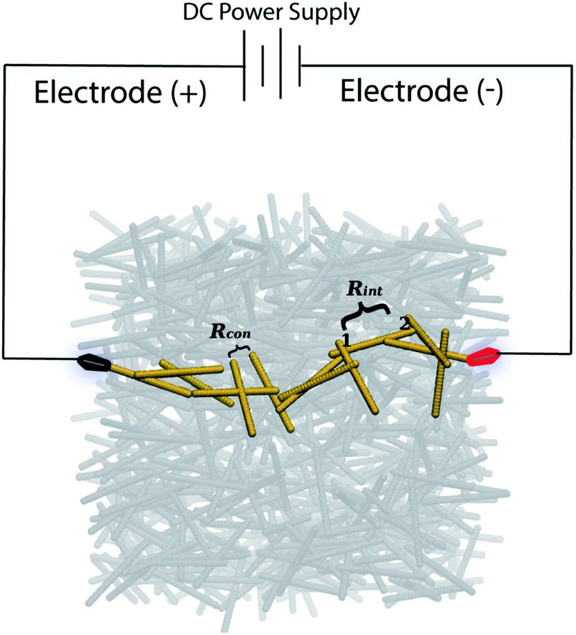 | ||
| Fig. 1 Schematic picture of the CNTs forming a conductive path. A continuous network of CNTs is formed when the percolation threshold is reached. To measure the Joule heating power, the sample is placed between two electrodes and an external potential is applied. A thermocouple allows to evaluate the temperature increase. Both electrical resistances contributions to the percolative path, the intrinsic (Rint) and contact one (Rcon), are emphasized. | ||
Joule heating takes place in conductive materials. In particular, composite materials switch from insulators to conductors once a critical concentration of the filler is reached (the so-called percolation threshold), that takes place when the filler concentration is sufficient to allow the formation of a continuous conductive path characterized by connected CNTs (schematically shown in Fig. 1).
The contributions to the percolative path are two: the intrinsic and contact resistances, described in the next subsection.
The percolative region is still very sensitive to small concentration variations or conformation changes, thus making the heat generation not efficient. Since it is required that the heat generated is stable for self-heating applications, the electrical conductivity has to be stable, and this condition is reached at filler contents about two times the percolation threshold.53,92 In this way it is ensured that the material is conductive and that small changes in CNT arrangement do not affect the conductive performances.
In Fig. 2, we schematically show the key concepts of the proposed approach for the calculation of Joule heating.
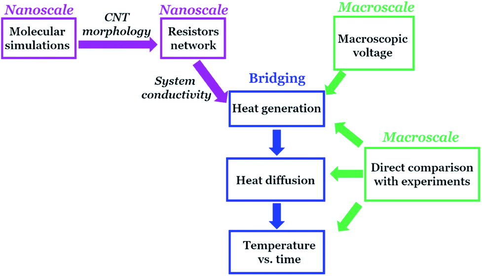 | ||
| Fig. 2 Schematic representation of the main ideas presented in this work. The proposed protocol aims to bridge the nano and macroscale. The nanoscopic explicit modeling of the material is needed to accurately simulate the Joule effect and heat diffusion, that is modeled by using a grid based picture allowing the connection to the macroscale, from which the external voltage is taken. In this schematic representation on the connecting arrows we underline the main quantities simulated at the nanoscale and transferred to the macroscale through the bridging grid picture. | ||
First of all, we propose to retain the molecular picture of the system, since it is important to properly include the different contributions to the overall resistance and so to properly simulate the system conductivity before evaluating the Joule heating and the heat diffusion. By using the hybrid particle-field MD simulation implemented in the OCCAM software,85–87 and whose main concepts and equations are presented in the ESI,† we are able to simulate different molecular configurations of assembled CNTs in the polymer matrix with a reasonable computational cost. We simulate a system on sizes of 100–200 nm, to obtain equilibrium morphology of CNTs about 28 nm long. Different filler concentrations are simulated to build the percolation curve and to verify which is the filler amount necessary for the Joule heating modeling, and then such curve is fitted by using the percolation law (more details in next sections). One of the main advantages of our approach is that we start from an explicit molecular picture of the system, and in agreement with this fact, the electrical resistances and conductivities are calculated explicitly as described in the following subsection.
 | (1) |
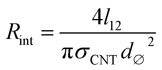
Electron ballistic tunneling through the contact junction causes the contact resistance, the second contribution (schematically shown in Fig. 1). Two separate CNTs can have multiple contacts: in our model CNTs are constructed as straight segments and each pair of non-adjacent segments produces contact resistance if the distance between them is less than dcutoff. The contact resistance can be approximated by the Landauer–Buttiker formula:94
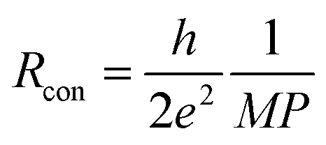 | (2) |
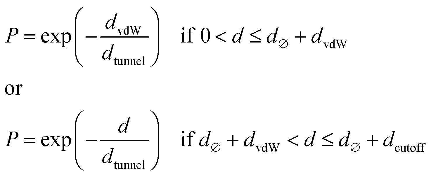 | (3) |
 is the minimum distance between two CNT segments where electron tunneling is most likely to occur, me is the electron mass, dvdW = 0.34 nm is the van der Waals separation distance and ΔE (1 eV) is the height of the barrier. The cutoff is calculated as dcutoff = 15dtunnel,84 and the transmutation probability is considered to be zero when the distance between two CNTs is d > dcutoff. Releasing the boundary conditions along one of the axis, two opposite faces of cuboids are formed and the conductivity of the resistor network between these faces may be calculated using the Kirchhoff circuit law:
 | (4) |
Solving the electric circuit has a huge computational cost and for these reasons different approaches have been employed. We chose to use the transfer-matrix method, successfully used and described in ref. 84 and 95, in this way the electrical conductivity of the simulated materials is obtained for different morphologies and at different CNT concentrations in order to build the percolative curve. This approach has been successfully applied to study electrical properties of CNT assemblies in homo and block copolymers in good agreement with several experimental findings.84
2.2 Molecular description of Joule heating
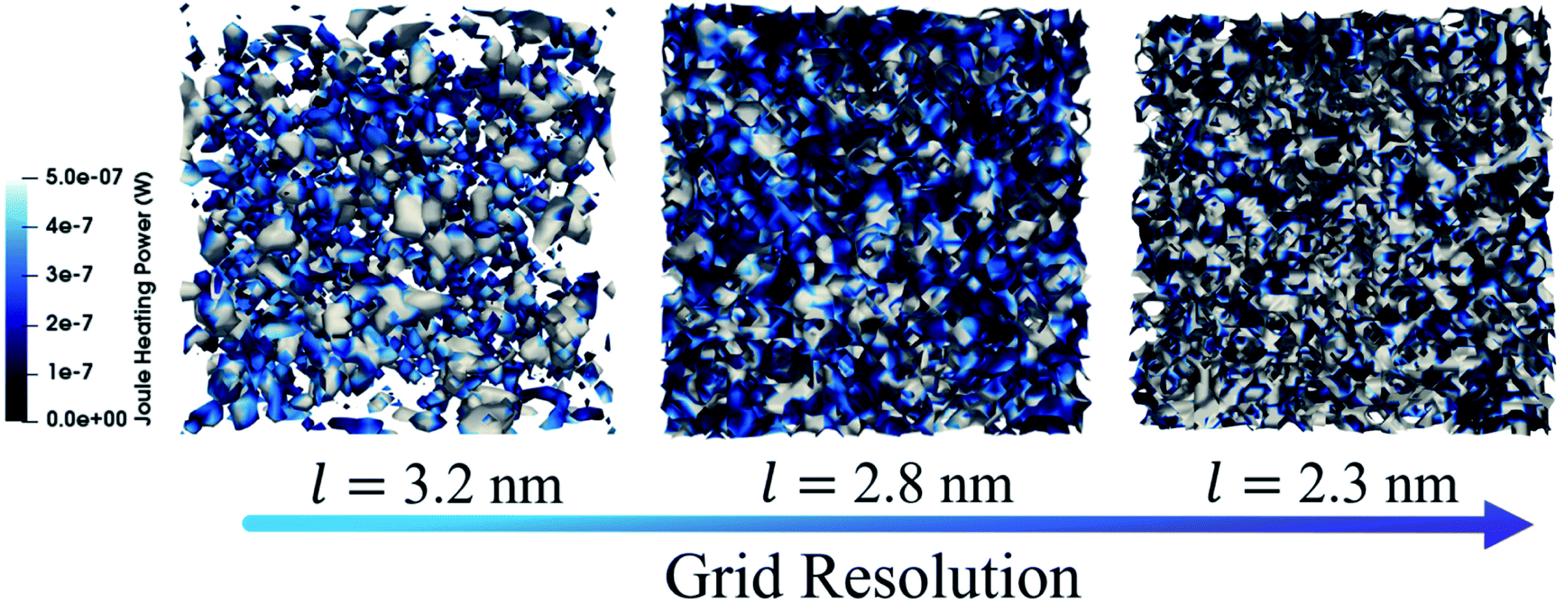
The key aspect of our proposed strategy is that the simulated Joule heating is obtained from an explicit representation of the system, and from this one the grid picture is built. We start from molecular configurations of the composite systems and on the basis of single beads positions the grid is built. In particular, this is done by using a procedure described in detail in the ESI,† in which a density scalar field accurately obtained from the particle positions is constructed. In this approach the density field is defined on the vertices of the cell where the particles are counted, allowing for a smoother and more detailed representation of the molecules positions. Indeed, fractions of a bead are assigned to a vertex on the basis of its position with respect to it (see SI for more details).This is a crucial step, since although a grid representation is employed to calculate Joule heating generation and heat diffusion, this one directly derives from an explicit molecular picture of the system under study, so a detailed map based on the particles position is obtained and an accurate description of the configuration is retained. This aspect is of key importance since it allows to not loose the role of the morphology of the material and to introduce it as an ingredient in the Joule heating evaluation. Differences among random, assembled or other morphologies are intrinsically retained thanks to this approach. The degree of accuracy used to build the grid can be decided and it affects how much detailed is the representation of the initial configuration in the grid picture. Of course, the accuracy is a compromise between the computational cost and the desired level of detail. A large grid is very convenient on a computational cost point of view, but it does not give a detailed representation of the configuration, retaining just a coarse picture of it where the molecular detail of the CNTs is lost. Small grids retain a huge level of detail where the actual nanotube configurations are not lost and an accurate information of the configuration is kept in the grid picture. In Fig. 3 we show some examples of the same CNT configuration represented with different grid sizes in which the different levels of accuracy and molecular detail reached in the different cases are evident and also the explicit coarse grained representation is shown (panel (b)). In panel (a) it is shown how a fine grid can approach to an atomistic picture of a CNT.
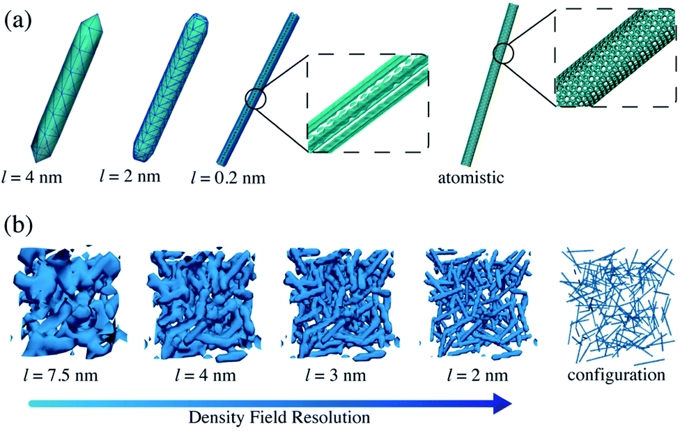 | ||
| Fig. 3 Panel (a) single CNT isodensity surface at different grid sizes and CNT atomistic picture. Panel (b) isodensity surfaces of CNTs in random conformation at different grid sizes. A snapshot of CNTs in coarse-grained representation is also shown to quantify the different degree of detail reached at different grid sizes. In the figure, l represents the grid length. | ||
2.3 Joule heating generation
In the proposed protocol, local electrical resistances are evaluated according to the local CNT concentration. These quantities are derived from electrical conductivities, calculated by using the percolation law shown in eqn (5):| σi/σCNT = η(fi − fc)τ | (5) |
| Fitted parameter | Random | Assembled (monomer) | Assembled (polymer) |
|---|---|---|---|
| η | 9.2 × 10⁻⁴ | 0.02 | 0.02 |
| f c | 2.8 | 1.89 | 1.84 |
| τ | 2 | 1.87 | 1.76 |
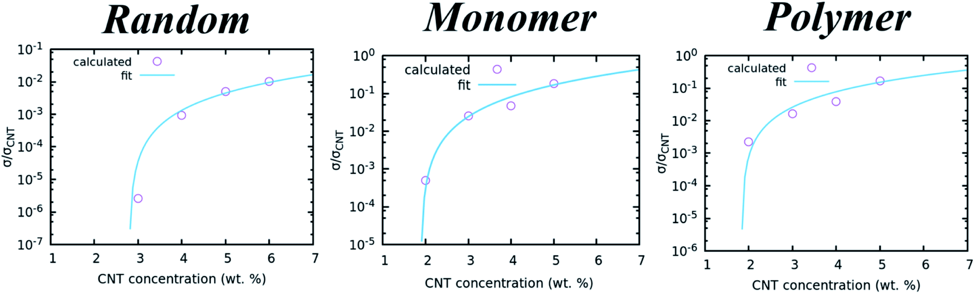 | ||
| Fig. 4 Calculated electrical conductivities at different CNT concentrations for the random and assembled in monomer and linear polymer matrices. The curves obtained by fitting the data with eqn (5) are also shown. | ||
From the results, it is clear that the critical concentration of randomly dispersed CNTs is around 2%, so for Joule heating applications we will employ concentrations higher than 2%, up to two times this one, while the critical concentration for the assembled morphologies is lower. This result suggests that lower concentrations of CNTs are necessary to build percolative paths when they are in assembled morphologies.
In our scheme the local conductivities are evaluated on grid points according to a grid scheme described in Fig. S1 of ESI.† On each grid point the conductivities are calculated by using eqn (5), where τ, η and fc are taken from Table 1. The simulation of the CNTs and polymer at CG level, has already shown to be accurate enough to simulate the electrical properties of such materials, validating the nanoscale as a crucial bridge to make comparisons with the macroscale.84
2.4 Joule heating calculation on the grid
The local electrical resistance, Ri (Ω), is calculated from the electrical conductivity as shown above for each grid element. This term is inversely proportional to the conductivity and is evaluated by using the grid geometrical parameters. The local heating power at grid point i (Pi, measured in watt) depends on the CNTs local density, and it is evaluated by using the heating power law:| Pi = Ii2Ri | (6) |
As shown for the isodensity surfaces, also the heating power is sensitive to the grid resolution. In Fig. 5 the Joule heating power is shown at different grid sizes. By switching from the coarser to the finer one, an increasing difference in colors intensity is observed. In particular, at the larger grid the difference among colors is less drastic, indeed not deep blue or white regions are observed while at finer grids this discrepancy is more emphasized and also the different color regions are smaller, indicating that locally different Joule heating powers are found. In general, larger heating power regions correspond to areas reacher in CNTs.
 | ||
| Fig. 5 Heating power isosurface at different grid resolutions. | ||
A direct comparison of our results can be done with experiments at the macroscale since we employ experimental external voltages, in this way the simulated quantities can give useful and applicable suggestions about material limits and possible improvements. The bridge between the nano and macroscale is given by the heat generation modeling since elements coming from the molecular size scale (explicitly modelled system, explicit resistor network modeling) are combined with macroscopic quantities (the applied voltage). This step is the crucial bridge between the nano and microscale since it allows to compare our results with experiments, because macroscopic voltage and percolation law are applied, but still keeping the molecular picture since it is implicitly embedded in the local density of the grid elements from which the Joule heating power is calculated. Once Pi is known, the heat generate (J) (see eqn (7)) can be evaluated according to the time interval in which the heating power is erogated:
| Qi = PiΔt | (7) |
| TJoule(i) = Qi/(cpmi) | (8) |
The obtained local temperatures are representative of the local filler concentration and provide also an indirect picture of the morphology and spatial arrangement of the conductor, as explicitly shown in Fig. 6. In this figure the isodensity surface of a composite material with CNTs in assembled morphology and with a concentration equal to 9% in weight in linear polymer matrix is shown along with local temperature isosurfaces after the application of an external potential difference.
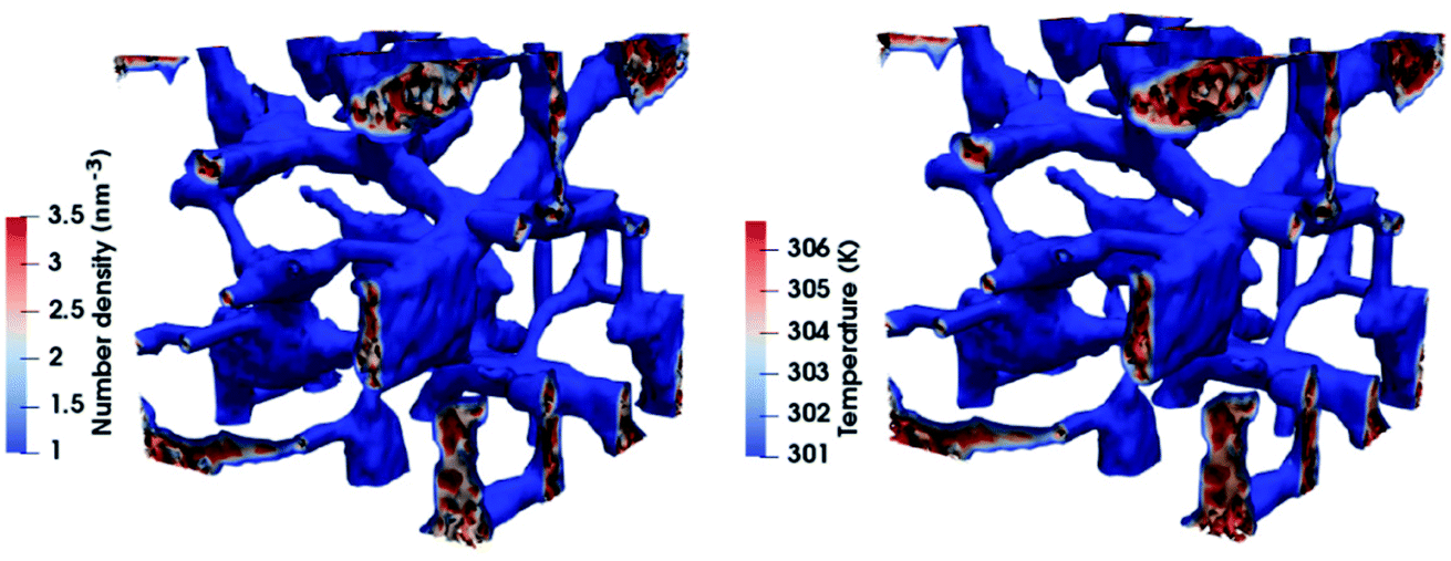 | ||
| Fig. 6 Isodensity surfaces of CNTs (9% in weight) in linear polymer assembled morphology (left panel) and temperatures isosurfaces (right panel) computed after the application of potential difference on that configuration. The employed grid size is 2.05 nm. | ||
The very clear correspondence between the CNT densities position (polymer densities are not shown for better clarity), and the local temperatures can be caught. Higher temperatures correspond to regions reacher in CNTs and the path formed by the local temperatures resemble exactly the one made by the densities. At this point a map of local heat generated by the system under study is known.
2.5 Modeling heat generation and diffusion
The local temperatures deviate from the macroscopic one imposed in the simulation because of the local Joule heating power due to the different local filler density calculated as described above, in each grid element vertex. To evaluate the heat diffusion, the heat diffusion equation has to be solved by including the extra term coming from the local Joule heat, and in the implemented scheme it is solved numerically by using the finite difference method approximation (second order central difference). This approach has been proposed and successfully employed to simulate Joule heating in metal single-crystal nanowires by Padgett and coworkers.72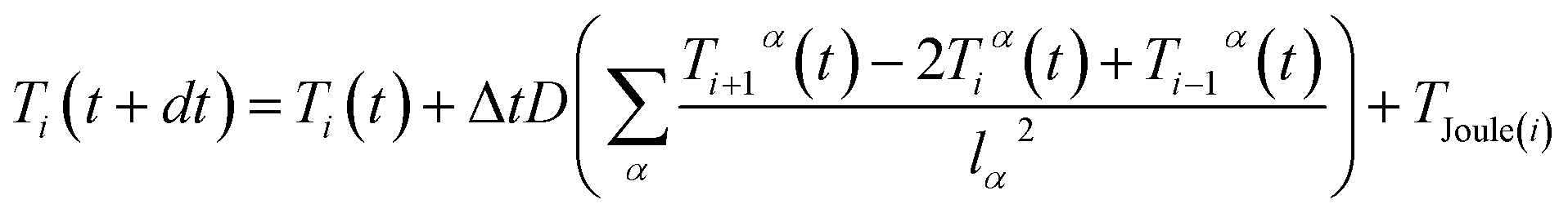 | (9) |
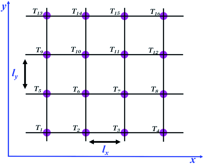 | ||
| Fig. 7 Simplified schematic 2D picture of a 4 × 4 grid to illustrate the grid scheme used to calculate local temperatures according to eqn (9) where the Joule heat contribution depending on the local CNT density is added. Temperatures are evaluated on the grid vertices. Periodic boundary conditions are applied in all directions. For this reason grid points 1 and 4, 5 and 8, 9 and 12, 13 and 16, 2 and 14, 3 and 15 are equivalent. | ||
This equation is solved iteratively and allows to follow the heat diffusion along the grid points. In our simulations we only consider the first part of the heat generation and diffusion without simulating its dissipation with the environment. However, this first part is the crucial one for the evaluation of the material capabilities to heat since it allows to understand how fast the materials are in increasing the temperature after the application of a potential difference. So, although we are already working on modeling also the cooling phase, the phenomena happening at early time remains the most important ones.
The heat diffusion is a fundamental aspect since it describes how the heat generated locally in the simulation box from the CNT diffuses in the system. On a practical point of view the efficiency of the heat diffusion is very important both in terms of how fast is the heat diffusion in the environment (represented by the heat conductivity coefficient) and in terms of its homogeneity, indeed although the heat generated depends on how much filler is present locally, it is important that the discrepancy between regions rich or poor of filler reaches the equilibrium in a small amount of time. The efficiency of the device is important because the de-ice function has to be as much homogeneous as possible in the material and should not depend on the microscopic distribution of the filler. This last aspect is ruled by the heat diffusion coefficient, of which two limits cases will be discussed below.
To simulate the diffusion of the heat due to the local temperature increase, the heat diffusion equation is employed according to eqn (9). Both local temperatures and the average system temperature are evaluated during the time. The system capability to heat, that represents the most important feature and quantity to evaluate the performance of the material, is finally calculated from the heating rate. It is obtained from the temporal evolution of the temperature, that is linear in the first stage of heat diffusion. In particular, for each step of the heat diffusion, the local temperatures are calculated on each grid vertex and averaged to obtain the temperature of the whole simulation box. The temperature against the time has, at the early stages of heat diffusion, a linear behavior (as shown in Fig. S2 and S3 of ESI†) and the heating rate is obtained as the slope of the fitted linear function. The heating rate calculation is the final most important output of the proposed method, and represents the most direct and immediate way to detect the limits or good performance of the chosen material.
The thermal diffusivity coefficient influences the homogeneity of the heat diffusion, i.e. it influences how fast an equilibrium temperature among the hot (rich in CNTs) and cold regions is reached. In particular, large values of D mean efficient diffusivity and fast homogeneity of temperature in the material and are typical of CNTs alone. Smaller values of D characterize composite material, where these can also be less than unity. In Fig. 8 it is shown a schematic picture of two limit cases.98
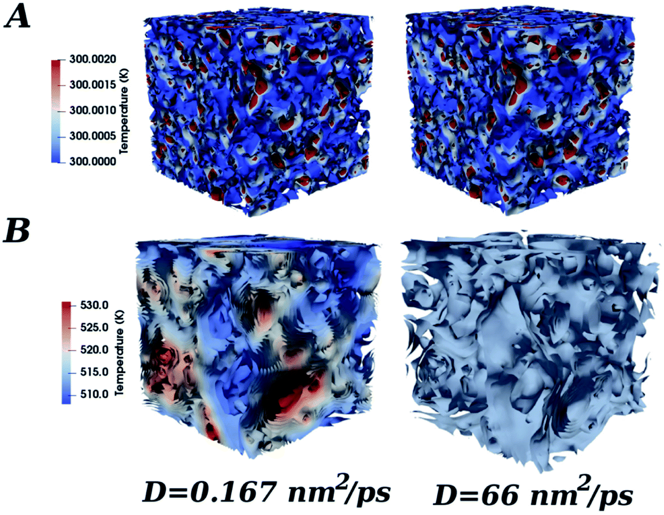 | ||
| Fig. 8 Temperature isosurfaces for randomly oriented CNTs (10% wt) showing local different temperatures depending on local different amount of nanotubes after the application of a potential difference of 1 V. Different temperatures are represented with colors from red (hotter regions, larger CNTs content) to blue (poor CNTs content). Panel (A) – the system is shown at the beginning of the simulation, performed by using a thermal diffusivity coefficient of 0.167 nm2 ps−1 (left) and 66 nm2 ps−1 (right). Panel (B) – the system is shown after 10.5 ns in which the heat diffusion has been simulated by using the same thermal diffusivity coefficients (0.167 nm2 ps−1 (left) and 66 nm2 ps−1 (right), respectively). A grid of 3.77 nm is employed in this case. | ||
The first one in which the heat diffusion equation is solved, a D value of 0.167 nm2 ps−1 is employed, while in the other case a value of 66 nm2 ps−1, similar to the ones of CNTs alone, is used. At the beginning of the simulation the system is substantially characterized by the same local temperatures, and very small differences are in agreement with the local filler concentration. As time passes the system starts to warm up, and after the same amount of simulation time that here is chosen 10.5 ns, it is observed that when the heat diffusivity is large, the temperature is the same in the whole simulation box while when smaller D values are employed, the local temperatures are still different and colder and warmer regions are observed. The heat diffusivity does not actually influence the average temperature of the system that in both cases is the same, but only the local temperature. So it is not an indicator of the total increase of the temperature during the time, but it indicates how homogeneous and how much time is necessary to have a homogeneous distribution of the macroscopic temperature.
2.6 Computational details
Regarding the Joule heating power calculation, the chosen grid to evaluate the local electrical conductivity is chosen to be about 37 nm. The parameters employed in eqn (5) are obtained by fitting the percolation curve calculated at different CNT concentrations. The time step for the heat diffusion is 200 ps, the thermal diffusivity is 1 nm2 ps−1 and the chosen CNT conductivity is of 1000 S m−1. To be employed at the nanoscale, the applied potential differences are scaled according to an average order of magnitude of the material dimensions employed in experiments, that we set to about 80 mm. The carbon nanotubes are about 28 nm long and have a diameter of 1.4 nm, the cubic simulation box length is 113.12 nm. The different compositions of the composite materials range from a CNT percentage of 1 to 10 in weight.3 Experimental section
In order to investigate the heating characteristics of the resin, the epoxy has been filled with Carbon nanotubes GRAPHISTRENGT C 100 supplied by Arkema. Thermogravimetric analysis (TGA) shows a carbon purity higher than 90% and a weight loss at 105 °C less than 1%. A detailed analysis of their morphology was performed using high-resolution transmission electron microscopy (HR-TEM). Carbon nanotubes resulted characterized by an external diameter between 10 and 15 nm, a length between 0.1 and 10 μm and a number of walls varying between 5 to 15. The filler has been embedded into the precursor (3,4-epoxycyclohexylmethyl-3′,4′-epoxycyclohexane carboxylate – ECC) by using an ultra-sonication for 20 min (Hielscher model UP200S-24 kHz high power ultrasonic probe). An amount of hardener (methyl hexahydrophthalic anhydride – MHHPA) has been added to filler/precursor mixture with a ratio by weight precursor/hardener of 1/1. The obtained mixtures have been mixed by magnetic stirring for 20 minutes at room temperature and subsequently degassed for 2 h at room temperature. The mixture has been cured by a triple curing cycle: 1 hour at 80 °C + 20 minutes at 120 °C + 1 hour at 180 °C. A concentration of 3% of the filler was used for electric heating measurement. A filler concentration of 3% has allowed obtaining a sample with a DC volume conductivity value of about 6.8 × 10⁻² S m−1. This result was obtained by electrical tests carried out in agreement with ref. 99. Regarding electric heating measurements, a data acquisition board (Thermocouple Data Logger supplied by Pico Technology) was used to acquire the thermocouples measurements. In order to record the local temperature evolution, a dedicated LabView software was developed. The temperatures were measured using a thin wire thermocouple (Type K Omega Engineering Ltd.) with negligible thermal inertia and an accuracy of ±0.5 °C which was positioned at the center of the rectangular geometry sample (81 × 56 × 4.5 mm3). The power supply EA-PSI 8360–10T (Elektro-Automatik, 0–360 V, 0–10 A, 1000 W max) was connected to the sample by two-wire contacts placed at the ends of the sample. In order to reduce possible effects due to surface roughness and to ensure an ohmic contact with the measuring electrodes, the samples were coated by using a silver paint with a thickness of about 50 μm and characterized by a surface resistivity of 0.001 Ω cm. All measurements were performed in direct current (DC) mode, with a selected constant power.4 Results and discussion
4.1 Morphology, filler concentration and voltage dependances
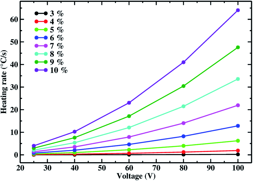
In this section, the implemented protocol to simulate Joule heating at the nanoscale is employed to investigate the dependance of the Joule heating power on the carbon nanotubes concentration, applied voltage and morphology.In Fig. 9 the heating rate (°C s−1) as function of the applied voltage is shown for systems with different CNT weight percentages in random orientation. In this case external macroscopic voltages of 25, 40, 60, 80 and 100 V are applied and the distribution of local temperatures, different for the Joule effect, is monitored. The heating rates are shown for CNT weight percentages from 3 to 10, while lower CNT contents are not considered since below or too close to the percolation threshold (that for the randomly oriented CNTs we found around 2%). Indeed, for CNT weight percentages below 3, no quantitative heat is produced, while at larger concentrations a clear change of behavior is observed. The drastic change in the heating rate is observed as the system overcomes the percolation threshold. This gap between the region below and above the percolation threshold is in agreement with the experiments, and with the fact that the formation of a percolative conductive network causes a neat transition of the system from insulator to conductor.56,100 As general trend we find that the heating rate increases as the applied voltage is higher for all the investigated CNT concentrations. In particular, from 3 to 10% of CNT, the sensitivity to the external voltage increases drastically, indeed while for a CNT concentration of 3% the heating rate does not overcome 1 °C s−1 even when an external voltage of 100 V is applied, while for a concentration of 10% the heating rate jumps from about 4 °C s−1 at 25 V to about 64 °C s−1 when 100 V are applied to the system.
 | ||
| Fig. 9 Heating rate for the random CNT configurations at different applied voltages. The heating rate is shown for different CNT concentrations. | ||
The information provided by our simulations can be very useful from a practical point of view, allowing to know in advance the performance dependance of a material on the applied voltage, and so to make a more accurate choice in practice. Moreover, the dependances on the voltage of different filler concentrations and the dispersion state of the filler, are also observed experimentally and the non linear correlation between the heating rate and applied voltage is in agreement with experimental trends.53,92 Of course the CNT concentration could be, in principle, further increased with respect to the ones shown in our study, but larger CNT contents could affect the mechanical features of the material and for this reason the choice of the best conditions for a satisfactory Joule heating is a compromise between efficiency and working conditions. In the presented cases there is no evidence of delamination or fracture, indicating that such CNT concentrations are not yet large enough to cause such damages.
It is very interesting to underline how the increase of the voltage enhances the discrepancies among the different filler concentrations, i.e. at 25 V there is not a huge gain in moving from a CNT content of 3% to 10%, while as the applied voltage increases, the different performance related to different conductive filler concentrations is emphasized. This fact means that, if low voltages are required for a specific application, materials with low CNT content can be chosen without drastically impact the reached heating rate, but it is not true when higher voltages are applied since in those cases a quantitative difference is found among the system compositions. This is also another useful information since, if high voltages can be employed, the choice of the material is not trivial because a huge gain is reached with higher CNT content. At 100 V the increasing discrepancy among the different filler concentrations is clear, showing that given an external voltage the improvement obtained by increasing the filler concentration is not of the same amount but increases always more as more filler is added. These trends showing the dependance on the applied voltage and different sensitivity of CNT concentrations to it, are reasonable and in qualitative agreement with experimentally found trends as further discussed later in this paper.
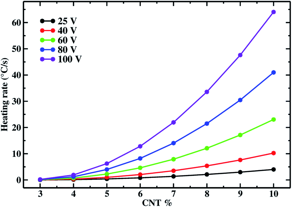
The effect of the applied voltage can be also observed from Fig. 10. In this figure, the heating rate is shown as function of the CNT% for the five different voltages. The drastic improvement of the Joule heating efficiency with the increase of the applied voltage is shown and the discrepancy as the CNT content increases is quantitative. The increase of the heating power depends on the larger current intensities reached when the system is percolated. Indeed, although the number of resistors increases with the filler content, since it depends on the local filler density according to eqn (5), also the global conductivity increases because of the larger number of contacts among CNTs, allowing to form the conductive network.
 | ||
| Fig. 10 Heating rate for the random CNT configurations at different CNT%. The heating rate is shown for different voltages. | ||
The reasonable trends found represent a test for the performance of the proposed computational approach, and the dependence on voltage and concentration are in agreement with experimental trends.61 In particular, the fact that larger heating rates are reached when the filler concentration is increased, and the quadratic dependence of the heating rate from the voltage that directly reflects the quadratic dependence on the heating power from the voltage, according to the equation P = V2/R. This last trend confirming that we are able to correctly simulate dependences observed at the macroscale. These trends represent also a systematic study that can be performed on such materials where factors affecting the heating performances can be disentangled and singularly analyzed.
In this section large heating rates are found compared with experimental results. To make a quantitative comparison with experiments it is necessary to properly treat and scale our data according to the different lengths of simulated and experimentally employed CNTs.
4.2 Comparison with experimental results
One of the main goals of this work is to propose a modeling strategy whose output information could be directly compared with experiments, and that can be employed to explain behaviors observed experimentally and help the rational design of self-heating nanomaterials. One of the main aspects giving rise to the gap between our model and the experimental data is the different scale. We simulate systems at the nanoscale where CNTs are about 28 nm long, that is a small size compared to the ones employed experimentally whose length ranges between 1–100 μm.53,61,92,100–104 Systems of sizes closer to the experimental one can be simulated, but at the cost of losing an accurate description of the main factors affecting and influencing the Joule effect. For this reason, in this work we chose to focus on a scale that allows us to perform wide screenings of parameters such as the interaction with the matrix, the nature of the matrix and the Joule effect measurement conditions like applied voltage, filler concentration, filler morphology. Our CNT model is a very simplified one, allowing us to simulate systems with about 106 particles, however building longer CNTs means to reach system sizes including about 109 particles and this would be too expensive on a computational point of view. Moreover, in order to avoid unphysical behaviors due to the periodic boundary conditions, the size of the simulation box has to be about four times the CNTs length, making the actual size of the system very large. However, compared to other simulation techniques based on an explicit representation of all the particle interactions (such as force field based molecular dynamics simulations), the hybrid particle-field approach allows to simulate larger systems otherwise not easily accessible.Because of the computational cost limits, the actual way to compare our results with experiments is to properly take into account the CNT length difference scaling quantities related to them. We employed CNT concentrations from 1 to 10% in weight while often these do not overcome 5% in weight in experiments. This discrepancy is mostly related to the different size of the CNTs, that can also be several μm long and wider in diameter compared to the ones employed in our modeling strategy.
To overcome this discrepancy, it is necessary to renormalize the physical quantities chosen to be compared. The first attempt is the connection between the different concentrations considered in the simulations (due to smaller lengths of the CNTs and the consequent larger percolation threshold, higher CNT concentrations are considered), and the experimental data usually reported in the literature. In this case, the most obvious choice is to renormalize the CNT content in terms of percolation threshold of the considered systems. In particular, the renormalized content of CNT is calculated as f/fc, so results of CNT percentages that are equivalent in relation with the percolative threshold (either calculated or experimental), are compared. Moreover, the Joule heating power is scaled for the ratio between the experimental and calculated percolation threshold to further take into account the difference in the quantity of heating source. This strategy to consider concentrations relative to the percolation threshold and to scale the heating rate for their ratio allows to compare our results with experimental ones directly taking into account the effect of the different dimensions, in particular the aspect ratio. Indeed, the aspect ratio has been shown to be directly connected to the percolation threshold and importantly affecting its value since it influences the geometrical mechanisms by which the conductive network is formed.6,15,84 Scaling for the percolation thresholds ratios allows to take into account the difference in simulated and experimental aspect ratio.
Following this proposed procedure we compare calculated heating rates with different experiments. In Table 2 our results (°C s−1) are compared with data from three different experiments where in all the cases the polymer matrices are thermoplastics and different voltages are applied. All the data shown in the table are also presented in Fig. 11.
| Voltage (V) | Random | Monomer | Polymer | Expt. (ref. 104) |
|---|---|---|---|---|
| 12 | 0.033 | 0.8 | 0.67 | 0.16 |
| 24 | 0.13 | 3.22 | 2.67 | 0.6 |
| Voltage (V) | Random | Monomer | Polymer | Expt. (ref. 103) |
|---|---|---|---|---|
| 15 | 0.052 | 1.26 | 1.04 | 1.5 |
| 17.5 | 0.071 | 1.71 | 1.42 | 2.05 |
| 20 | 0.092 | 2.24 | 1.85 | 3.28 |
| Voltage (V) | Random | Monomer | Polymer | Expt. (ref. 102) |
|---|---|---|---|---|
| 30 | 0.17 | 4.28 | 3.55 | 0.78 |
| 40 | 0.31 | 7.6 | 6.32 | 2.33 |
| 50 | 0.48 | 11.88 | 9.87 | 3.88 |
| 60 | 0.69 | 17.11 | 14.12 | 5.43 |
| 70 | 0.94 | 23.28 | 19.35 | 7.75 |
| 80 | 1.23 | 30.42 | 23.28 | 10.08 |
| 90 | 1.56 | 38.49 | 31.99 | 13.18 |
| 100 | 1.92 | 47.52 | 39.49 | 16.28 |
 | ||
| Fig. 11 Heating rates simulated vs. experimental at different voltages. Simulated results are shown for CNTs in random, monomer and linear polymer phase. Snapshots of these morphologies are also shown. The polymer phase is not shown to better emphasize the different CNTs arrangements. Experimental values are those discussed in Table 2 from ref. 102–104. For the simulated data the error of the fitted heating rates, obtained by a least squares fitting procedure, is within the point size of the figure. | ||
The first comparison is with experiments performed by Dorigato and coworkers (ref. 104), where they employ poly(butylene terephthalate) as polymer matrix, CNTs are 1.5 μm long with a diameter of 9.5 nm, and potential differences of 12 and 24 V are applied. They find a percolation threshold lower than 0.5% wt (much smaller than those we found for simulated materials) and in the table we report experimental heating rates evaluated for composites having a CNT concentration of 3% wt, suggesting that a filler concentration at least six times larger than the critical one is employed. To compare the heating rates of simulated composites it is necessary to consider concentrations larger than the percolative threshold of about the same amount, so for the random morphology we choose a CNT concentration of 10% wt (percolation threshold 2.8), and for the monomer and linear polymer we choose 9% wt (percolation thresholds 1.89 and 1.84% wt, respectively). From the calculated heating rates it is observed that experimental values are intermediate between the random (lower limit) and assembled (upper limits) ones. This result suggests that in this case it is possible to hypotesize that the experimental morphology could be intermediate between a random one in which the contacts among CNTs are not optimized, and the assembled ones where the intermolecular contacts among CNTs are maximized.
A quite different scenario is found when data from Sangroniz and coworkers (ref. 103) are analyzed. In this case experimental polymer matrix is polypropylene and CNTs are about 10–20 μm long with a diameter of 30–50 nm, however they do not explicitly report the percolative concentration and for heating rates measurements they use a filler concentration of 5% wt, stating that it is an already percolated network. So, to make sure to be enoughly beyond the percolative threshold, also in this case we chose CNTs concentrations of 10% wt for random and 9% wt for assembled morphologies. For all the three voltages (15, 17.5 and 20 V), heating rates of assembled morphologies are closer to the experimental ones suggesting that probably in this case morphologies obtained from Sangroniz and coworkers resemble more the assembled ones.
Finally, Jeong et al. (ref. 102) measure heating rates in a wide range of voltages, and we compare calculated ones in the range of 30–100 V for a filler concentration about six times the critical one (in agreement with CNT concentrations chosen in their work). Their polymer matrix is poly(m-phenylene isophthalmide) and CNTs are about 100 μm long with a diameter of about 10–15 nm. For all the potential differences applied, experimental heating rates are intermediate between random and assembled morphologies (as clearly observed in Fig. 11). It is interesting to observe how this discrepancy increases with the applied voltage, indeed at 30 V the random morphology is closer to the experimental value compared to the other two, and in general for all the three morphologies the discrepancies are more pronounced at higher voltages. This fact is in agreement with the trends discussed in the previous section in which we showed that, for a given concentration, material performances diverge when larger voltages are applied (Fig. 9). Another interesting aspect is the non linear behavior of the heating rate as function of the voltage for both calculated and experimental curves (for the random case it is just not easily caught because of the scale). This trend can be associated to the quadratic dependance of the electric power from the voltage (P = V2/R) that is dissipated as Joule heating (eqn (8)). Indeed, the heating rate is obtained from the temperature change during the time in the material, and is a direct expression of the Joule heating (and so of the electric power, eqn (6)) since the only source of temperature change comes from the electrically conductive fillers (see eqn (9)), allowing the quadratic behavior to be observed also here. This result confirms the behavior of the composite material as a classical ohmic conductor, and the fact that it is observed also in the simulated heating rates suggests that the proposed model is able to catch its nature.
In Table 3 we make a comparison with other experiments where the matrix is in all cases a resin. Both experimental and computed data are also shown in Fig. 13.
| Voltage (V) | Random | Monomer | Polymer | Expt. (ref. 100) |
|---|---|---|---|---|
| 25 | 0.014 | 0.11 | 0.18 | 0.0167 |
| 60 | 0.081 | 0.65 | 1.04 | 0.2 |
| 100 | 0.22 | 1.8 | 2.89 | 0.62 |
| Voltage (V) | Random | Monomer | Polymer | Expt. (ref. 101) |
|---|---|---|---|---|
| 140 | 0.44 | 3.52 | 5.68 | 0.85 |
| Voltage (V) | Random | Monomer | Polymer | Expt. (this work) |
|---|---|---|---|---|
| 67 | 0.1 | 0.81 | 1.29 | 0.082 |
| 83 | 0.15 | 1.24 | 1.99 | 0.13 |
| 108 | 0.26 | 2.09 | 3.38 | 0.21 |
In Prolongo and coworkers experiments (ref. 100), CNTs have an average length of about 1 μm and a diameter of about 9.5 nm, the polymer matrix is an epoxy resin (epoxy diglycidil-ether bisphenol-A with 4,4′-diaminodiphenyl sulfone) and heating rates are calculated at 25, 60 and 100 V. They find that the critical concentration of their system is about 0.1% in weight of CNTs, and the data we compared with are those of a composite with a CNT concentration of 0.25% wt, that is about two times and half the percolative one. So, for all these cases we employed systems with 5% wt in CNTs for the random and 3% wt for the assembled morphologies to calculate heating rates. The simulated values show a good agreement with experimental ones, we are able to reproduce the same order of magnitude of macroscopic experiments. These results underline the importance of properly scaling the quantities obtained from the simulation when a direct comparison with experiments is performed. When comparing the cases of CNTs in assembled morphology in monomer and in linear polymer matrix, the simulated heating rates are larger than the experimental ones. The experimental values are closer to the random morphology, that slightly underestimates the heating rate while monomer and linear polymer phase morphologies are more performing. This fact could suggest that a random like dispersion is probably obtained in the epoxy resin matrix that does not allow the CNTs to arrange in a way that could improve the number of contacts.
In the case of Neitzert and coworkers (ref. 101), the applied external voltage is 140 V, CNTs length ranges from 0.1–10 μm with a diameter of about 10 nm and the polymer matrix is an epoxy resin (epoxy diglycidil-ether bisphenol-A with 4,4′-diaminodiphenyl sulfone). The authors do not explicitly report the percolation threshold, and they state that 0.5% wt in CNTs (used in the experiment) is large enough to measure Joule heating properties, so we chose a system with a CNT concentration about two times the percolation threshold to make sure that the material is sufficiently beyond the percolation threshold. The heating rate calculated at random conformation is lower than the experimental value (0.44 vs. 0.85 °C s−1), while the assembled morphology in linear polymer is larger than it (5.68 °C s−1), although in both cases the same order of magnitude of the experiment is reproduced, showing that the proposed scaling is efficient to allow a direct comparison with experimental data. As also found in the previous comparison, also in this case the trends underline that for an assembled case there is a maximally optimized structure for the formation of a percolative path compared to the random case and possibly, since both of them are ideal cases, the actual experimental conformation could be intermediate between the two limiting cases, as suggests the heating rate value laying between the two calculated ones.
In the assembled cases the CNT conductive networks are optimized and the maximum number of connections among the nanotubes is reached. As shown in Fig. 12, the CNTs create bundle structures.
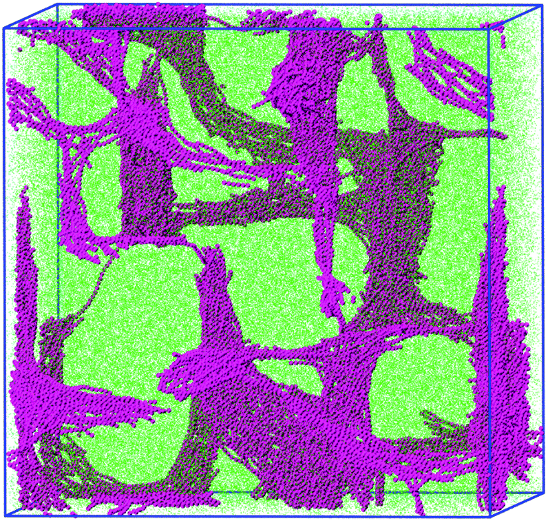 | ||
| Fig. 12 Schematic picture of a configuration of the composite system composed by CNTs (magenta, beads representation) at 8% in weight and the polymer matrix (green, points representation) in an assembled morphology after running a molecular dynamics simulation starting from a random configuration. It is clear the presence of CNT bundles forming percolative networks. | ||
Moreover, for assembled morphologies the percolation threshold is reached at lower CNT content, as also shown in ref. 84, allowing to use a smaller content of CNT in the composite material with the advantage to have a less expensive material (lower content of CNT) and also affecting less the mechanical properties of the resin.
It is interesting that when CNTs are assembled in monomer, the heating rate is slightly lower than the assembled in linear polymer (3.52 °C s−1), suggesting that the electric circuit is more optimized if compared with random case, creating optimized connections at the nanoscale, although not efficient enough like the case in linear polymer matrix. The case in which CNTs are assembled in monomer represents an intermediate stage, in terms of efficiency, between the random and assembled in linear polymer morphology where a more structured (and so similar to the assembled in linear polymer one) phase is already reached. The heating rate values are indeed more similar to the assembled than to the random ones. This trend is not observed at larger filler concentrations where also the assembled morphology in monomer is more performing (as observed in the comparison with thermoplastic matrices). These trends could be related to the fact that at low concentrations, although a CNTs structuration better than the one in the random case is reached, the number of contacts is not large enough to improve the performance and optimize the electric circuit, while at larger filler concentrations the nanostructuration created by CNTs has a much larger number of contributions, allowing the advantages of this structuration to emerge and also to overcome the performance in linear polymer where, although the formation of well-defined domains rich in CNTs, it is the monomer to appear a more ideal situation, also thanks to the larger mobility freedom of CNTs in monomer matrix compared to a more confined situation as in linear polymer.
Calculated heating rates have also been compared with experiments performed in this work at 67, 83 and 108 V (as shown in Table 3). These Joule heating rate experimental measurements have been performed to have more data in the 60–110 voltage range to compare with simulated results and to further corroborate the good behavior of the proposed model. Also in this case we perform a direct comparison with experiments, by using the experimental voltage on the nanoscale, and we are able to have very good agreement with experimental heating rate. As in the other cases, the system compositions chosen for the assembled in monomer and linear polymer phase cases have a CNT content of 3% while for the random case it is 5% since these concentrations are about two times the respective percolative thresholds. The random case compared with the other two, shows heating rate values very close to the experimental values suggesting that probably the experimental CNTs resemble a random like dispersion.
Finally, in Fig. 13 we also show heating rates calculated for 12 and 170 V, using composites with the same CNT contents employed above, to further emphasize that discrepancies among heating rates of different morphologies increase with increasing voltages (as also found in the discussion of systems with thermoplastic matrices).
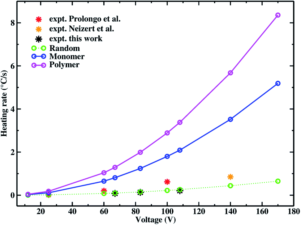 | ||
| Fig. 13 Heating rates simulated vs. experimental at different voltages. Simulated results are shown for CNTs in random, monomer and linear polymer phase. Experimental values are those discussed in Table 3 from ref. 100, 101 and this work. The error of the fitted heating rates, obtained by a least squares fitting procedure, is within the point size of the figure for both calculated and experimental data. | ||
All the collected information can be very helpful since underline the role of morphology of CNT assemblies in the performance of such materials, and how important can be the fabrication and optimization of the resistor network.
Simulated data suggest that the experimental heating rates obtained for all the considered thermosetting resins reflect materials with a morphology generally closer to a random assembly of CNTs. So, our simulation catches an important information, where from the electrical and thermal conduction behavior of the material we can disentangle the actual morphology behind it.
The information collected for both thermoplastic polymers and epoxy resins could be a precious information since it can drive experimentalists toward a finer an better design of the materials and also to understand the chemical reasons of different electrical and thermal performances. These information can only be reached at the nanoscale since it is the scale at which the assembly of the CNTs takes place. More detailed information and understanding of the materials can be done by increasing the specificity of the chosen model, especially to simulate different polymer matrices and so to investigate behaviors that are characteristic of a chosen material. However, these general trends give an important insight to disentangle the complexity hidden behind different materials.
5 Conclusions and perspectives
In this paper a modeling protocol to simulate Joule effect on composite materials at the nanoscale, is presented. Joule heating is a promising feature characterizing composite materials made of a polymer matrix and a carbon-based conductive filler, since it can be used for many innovative applications such as self-deicing, self-curing, in different fields such as aeronautics, automotive or civil engineering. The nanoscale picture represents a bridge between the molecular picture, employed to build the modelled materials, and the macroscopic one, where a mesh-based approach is used to simulate Joule heating power and heat diffusion. This scale has shown to be crucial to retain an explicit picture of the material and to allow to reach large size and time scales comparable with the experimental ones. The novelty in the proposed computational approach is its capability to retain the explicit picture of the simulated systems, that we have shown to be necessary to catch the behavior of different morphologies, and at the same time be able to compare simulated results with experimental ones by properly taking into account the different size and time scales. In this way the computational limits due to the necessity to retain the explicit simulation of the system are overcome. In this way our proposed protocol can be helpful to both analyze and disentangle the main factors influencing the heating capabilities of the materials and also make previsions on their behaviors. Heating rates dependances on material morphology, concentration, applied voltage and also heat diffusion coefficient are analyzed. Our simulations shed light on the specific dependence on the voltage of the different morphologies. Indeed, we find that assembled morphologies are more sensitive to the voltage with respect to random ones, showing larger heating rates. These results allow to give insights on the morphology of the CNTs network on the basis of the different sensitivity to the applied voltage. Direct comparisons with different experimental case studies have been investigated and good agreement with experimental findings is obtained. A very important role in the self-heating properties is played by the CNTs assemblies in different situations. In particular, dendritic nanostructures formed when CNTs are assembled in the organic matrices, lead to optimal arrangements that increase conductivities with respect to ideal homogeneous CNTs distributions. Different CNTs assemblies in nanomaterials based on thermoplastic (intermediate between dendritic and random arrangements) or thermosetting (very close to random arrangements) matrices can explain the different performances of these two class of nanocomposites.Conflicts of interest
There are no conflicts to declare.Acknowledgements
G. Donati and G. Milano gratefully acknowledge the European Union Horizon 2020 Programme, under Grant Agreement No. 760940 (MASTRO) for financial support. The computing resources and related technical support used for this work have been provided by CRESCO/ENEAGRID High Performance Computing infrastructure and its staff. CRESCO/ENEAGRID High Performance Computing Infrastructure is founded by ENEA, the Italian National Agency for New Technologies and by Italian and European research programs, see http://www.cresco.enea.it/english for information. G. Donati and G. Milano thank Professor Roberto Pantani from the Department of Engineering at the University of Salerno for very useful discussions.Notes and references
- R. Bogue, Assembly Autom., 2012, 32, 3–7 CrossRef.
- R. Bogue, Assembly Autom., 2014, 34, 16–22 CrossRef.
- A. Raza, U. Hayat, T. Rasheed, M. Bilal and H. M. N. Iqbal, J. Mater. Res. Technol., 2019, 8, 1497–1509 CrossRef CAS.
- S. Rana, P. Subramani, R. Fangueiro and A. G. Correia, AIMS Mater. Sci., 2016, 3, 357–379 CAS.
- Z. X. Khoo, J. E. M. Teoh, Y. Liu, C. K. Chua, S. Yang, J. An, K. F. Leong and W. Y. Yeong, Virtual Phys. Prototyp., 2015, 10, 103–122 CrossRef.
- W. Bauhofer and J. Z. Kovacs, Compos. Sci. Technol., 2009, 69, 1486–1498 CrossRef CAS.
- C. W. Nan, Y. Shen and J. Ma, Annu. Rev. Mater. Res., 2010, 40, 131–151 CrossRef CAS.
- R. M. Mutiso and K. I. Winey, Prog. Polym. Sci., 2015, 40, 63–84 CrossRef CAS.
- X. Yu, H. Cheng, M. Zhang, Y. Zhao, L. Qu and G. Shi, Nat. Rev. Mater., 2017, 2, 17046 CrossRef CAS.
- W. Obitayo and T. Liu, J. Sens., 2012, 2012, 1–15 CrossRef.
- I. Kang, Y. Y. Heung, J. H. Kim, J. W. Lee, R. Gollapudi, S. Subramaniam, S. Narasimhadevara, D. Hurd, G. R. Kirikera, V. Shanov, M. J. Schulz, D. Shi, J. Boerio, S. Mall and M. Ruggles-Wren, Composites, Part B, 2006, 37, 382–394 CrossRef.
- J. N. Coleman, S. Curran, A. B. Dalton, A. P. Davey, B. McCarthy, W. Blau and R. C. Barklie, Phys. Rev. B: Condens. Matter Mater. Phys., 1998, 58, R7492–R7495 CrossRef CAS.
- M. Moniruzzaman and K. I. Winey, Macromolecules, 2006, 39, 5194–5205 CrossRef CAS.
- M. Bryning, M. F. Islam, J. M. Kikkawa and A. G. Yodh, Adv. Mater., 2005, 17, 1186–1191 CrossRef CAS.
- J. Li, P. C. Ma, W. S. Chow, C. K. To, B. Z. Tang and J. K. Kim, Adv. Funct. Mater., 2007, 17, 3207–3215 CrossRef CAS.
- R. Ramasubramaniam and J. Chen, Appl. Phys. Lett., 2003, 83, 2928–2930 CrossRef CAS.
- F. Du, J. E. Fischer and K. I. Winey, J. Polym. Sci., Part B: Polym. Phys., 2003, 41, 3333–3338 CrossRef CAS.
- J. G. Meier, C. Crespo, J. L. Pelegay, P. Castell, R. Sainz, W. K. Maser and A. M. Benito, Polymer, 2011, 52, 1788–1796 CrossRef CAS.
- D. Stauffer and A. Aharony, Introduction to Percolation Theory, Taylor and Francis, London, 1992 Search PubMed.
- J. Hoshen and R. Kopelman, Phys. Rev. B: Condens. Matter Mater. Phys., 1976, 14, 3438–3445 CrossRef CAS.
- R. Zallen, The Physics of Amorphous Solids, Wiley, New York, 1983 Search PubMed.
- D. J. Bergman and Y. Imry, Phys. Rev. Lett., 1977, 39, 1222–1225 CrossRef.
- C. Nan, Prog. Mater. Sci., 1993, 37, 1–116 CrossRef CAS.
- S. Stankovich, D. A. Dikin, G. H. B. Dommett, K. M. Kohlhaas, E. J. Zimney, E. A. Stach, R. D. Piner, S. T. Nguyen and R. S. Ruoff, Nature, 2006, 442, 282–286 CrossRef CAS PubMed.
- A. V. Kyrylyuk, M. C. Hermant, T. Schilling, B. Klumperman, C. E. Koning and P. V. D. Schoot, Nat. Nanotechnol., 2011, 6, 364–369 CrossRef CAS PubMed.
- R. H. J. Otten and P. V. D. Schoot, J. Chem. Phys., 2011, 134, 094902 CrossRef PubMed.
- R. H. J. Otten and P. V. D. Schoot, Phys. Rev. Lett., 2009, 103, 225704 CrossRef PubMed.
- S. H. Jang, D. Kim and Y. Park, Materials, 2018, 11, 1775 CrossRef PubMed.
- A. Moisala, Q. Li, I. A. Kinloch and A. H. Windle, Compos. Sci. Technol., 2006, 66, 1285–1288 CrossRef CAS.
- K. Wang, K. Chizari, I. Janowska, S. M. Moldovan, O. Ersen, A. Bonnefront, E. R. Savinova, L. D. Nguyen and C. Pham-Huu, Appl. Catal., A, 2011, 392, 238–247 CrossRef CAS.
- E. Esmizadeth, A. A. Yousefi and G. Naderi, Iran. Polym. J., 2015, 24, 1–12 CrossRef.
- R. H. Baughman, A. A. Zakhidov and W. A. de Heer, Sci. Mag., 2002, 297, 787–792 CAS.
- L. Guadagno, L. Vertuccio, A. Sorrentino, M. Raimondo, C. Naddeo, V. Vittoria, G. Iannuzzo, E. Calvi and S. Russo, Carbon, 2009, 47, 2419–2430 CrossRef CAS.
- B. Mas, J. P. Fernandez-Blazquez, J. Duval, H. Bunyan and J. J. Vilatela, Carbon, 2013, 63, 523–529 CrossRef CAS.
- J. K. Sandler, J. E. Kirk, I. A. Kinloch, M. S. Shaffer and A. H. Windle, Adv. Mater., 2003, 44, 5893–5899 CAS.
- S. Stankovich, D. A. Dikin, G. H. Dommett, K. M. Kohlhass, E. J. Zimney and E. A. Stach, Nature, 2006, 442, 282–286 CrossRef CAS PubMed.
- L. Guadagno, B. D. Vivo, A. D. Bartolomeo, P. Lamberti, A. Sorrentino, V. Tucci, L. Vertuccio and V. Vittoria, Carbon, 2011, 49, 1919–1930 CrossRef CAS.
- D. Yoo, S. Kim, M. Kim, D. Kim and H. Shin, J. Mater. Res. Technol., 2019, 8, 827 CrossRef CAS.
- M. J. Khattak, A. Khattab and H. R. Rizvi, Constr. Build. Mater., 2013, 40, 738 CrossRef.
- O. Galao, L. Baiñón, F. J. Baeza, J. Carmona and P. Gracés, Materials, 2016, 9, 281 CrossRef PubMed.
- T. Ragab and C. Basaran, J. Appl. Phys., 2009, 106, 063705 CrossRef.
- A. Heinrich, R. Ross, G. Zumwalt, J. Provorse and V. Padmanabhan, Aircraft Icing Handbook, Gates Learjet Corp., Wichita, KS, 1991, vol. 2 Search PubMed.
- O. Parent and A. Ilinca, Cold Reg. Sci. Technol., 2011, 65, 88–96 CrossRef.
- R. H. Strehlow and R. Moser, SAE, 2009, 2009-01-3165 Search PubMed.
- L. Vertuccio, F. D. Santis, R. Pantani, K. Lafdi and L. Guadagno, Composites, Part B, 2019, 162, 600–610 CrossRef CAS.
- B. G. Falzon, S. Frenz and B. Gilbert, Composites, Part A, 2015, 68, 323–325 CrossRef CAS.
- J. Sloan, High Perform. Compos., 2009, 17, 27–29 Search PubMed.
- C. Li, X. Cui, Z. Wu, J. Zeng and S. Xing, Adv. Mater. Res., 2013, 1322–1325 CAS.
- X. Yao, S. C. Hawkins and B. G. Falzon, Carbon, 2018, 130–138 CrossRef CAS.
- T. Wang, Y. Zheng, A.-R. O. Raji, Y. Li, W. K. Sikkema and J. M. Tour, ACS Appl. Mater. Interfaces, 2016, 8, 14169–14173 CrossRef CAS PubMed.
- M. Mohseni and A. Amirfazli, Cold Reg. Sci. Technol., 2013, 87, 47–58 CrossRef.
- N. Karim, M. Zhang, S. Afroj, V. Koncherry, P. Potluri and K. S. Novoselov, RSC Adv., 2018, 8, 16815 RSC.
- S. H. Jang and Y. L. Park, Nanomater. Nanotechnol., 2018, 8, 1–8 CrossRef.
- D. D. L. Chung, Smart Mater. Struct., 2004, 13, 562–565 CrossRef CAS.
- T. Bayerl, M. Duhovic, P. Mitschang and D. Bhattachayya, Composites, Part A, 2014, 57, 27–40 CrossRef CAS.
- S. G. Prolongo, R. Moriche, G. D. Rosario, A. Jimenez-Suarez, M. G. Prolongo and A. Urena, J. Polym. Res., 2016, 23, 189 CrossRef.
- Y. N. Kong, P. M. Wang, S. H. Liu, G. R. Zhao and Y. Peng, Materials, 2016, 9, 733 CrossRef PubMed.
- T. Ragab and C. Basaran, Phys. Lett. A, 2010, 374, 2475–2479 CrossRef CAS.
- P. Gautreau, T. Ragab and C. Basaran, J. Appl. Phys., 2012, 112, 103527 CrossRef.
- J. G. Park, Q. Cheng, J. Lu, J. Bao, S. Li, Y. Tian, Z. Liang, C. Zhang and B. Wang, Carbon, 2012, 50, 2083–2090 CrossRef CAS.
- F. X. Wang, W. Y. Liang, Z. Q. Wang, B. Yang, L. He and K. Zhang, eXPRESS Polym. Lett., 2018, 12, 285–295 CrossRef CAS.
- B. Willocq, R. K. Bose, F. Khelifa, S. J. Garcia, P. Dubios and J. Raques, J. Mater. Chem. A, 2016, 4, 4089 RSC.
- G. Donati, A. Petrone, P. Caruso and N. Rega, Chem. Sci., 2018, 9, 1126 RSC.
- G. Donati, D. B. Lingerfelt, C. M. Aikens and X. Li, J. Phys. Chem. C, 2018, 122, 10621 CrossRef CAS.
- G. Donati, D. B. Lingerfelt, C. M. Aikens and X. Li, J. Phys. Chem. C, 2017, 121, 15368 CrossRef CAS.
- A. Wildman, G. Donati, F. Lipparini, B. Mennucci and X. Li, J. Chem. Theory Comput., 2019, 15, 43 CrossRef CAS PubMed.
- G. Donati, D. B. Lingerfelt, A. Petrone, N. Rega and X. Li, J. Phys. Chem. A, 2016, 120, 7255 CrossRef CAS PubMed.
- A. Petrone, P. Cimino, G. Donati, H. P. Hratchian, M. J. Frisch and N. Rega, J. Chem. Theory Comput., 2016, 12, 4925 CrossRef CAS PubMed.
- R. L. Goff, N. Boyard, V. Sobotka and D. Delaunay, Int. J. Material Form., 2010, 3, 805 CrossRef.
- W. L. V. Price, Build. Environ., 1983, 18, 219–222 CrossRef.
- S. K. Thangaraju and K. M. Munisamy, IOP Conf. Ser.: Mater. Sci. Eng., 2015, 88, 012036 Search PubMed.
- C. W. Padgett and D. W. Brenner, Mol. Simul., 2005, 31, 749–757 CrossRef CAS.
- J. D. Schall, C. W. Padgett and D. W. Brenner, Mol. Simul., 2005, 31, 283–288 CrossRef CAS.
- D. L. Irving, C. W. Padgett and D. W. Brenner, Modell. Simul. Mater. Sci. Eng., 2009, 17, 015004 CrossRef.
- M. Alaghemandi, F. Müller-Plathe and M. C. Böhm, J. Chem. Phys., 2011, 135, 184905 CrossRef PubMed.
- Y. Gao and F. Müller-Plathe, J. Phys. Chem. B, 2016, 120, 1336–1346 CrossRef CAS PubMed.
- Y. Gao and F. Müller-Plathe, J. Phys. Chem. C, 2018, 122, 1412–1421 CrossRef CAS.
- M. Alaghemandi, E. Algaer, M. C. Böhm and F. Müller-Plathe, Nanotechnology, 2009, 20, 115704 CrossRef PubMed.
- Y. Gao and F. Müller-Plathe, Polymer, 2017, 129, 228–234 CrossRef CAS.
- Z. Han and A. Fina, Prog. Polym. Sci., 2011, 36, 914–944 CrossRef CAS.
- J. Che, T. Cagin and W. A. Goddard III, Nanotechnology, 2000, 11, 12237 CrossRef.
- J. Hone, Carbon Nanotubes: Thermal Properties, 2004 Search PubMed.
- N. R. Pradhan, H. Duan, J. Liang and G. S. Iannaccione, Nanotechnology, 2009, 20, 245705 CrossRef CAS PubMed.
- Y. Zhao, M. Byshkin, Y. Cong, T. Kawakatsu, L. Guadagno, A. D. Nicola, N. Yu, G. Milano and B. Dong, Nanoscale, 2016, 8, 15538 RSC.
- G. Milano and T. Kawakatsu, J. Chem. Phys., 2009, 130, 214106 CrossRef PubMed.
- G. Milano and T. Kawakatsu, J. Chem. Phys., 2010, 133, 214102 CrossRef PubMed.
- Y. Zhao, A. De Nicola, T. Kawakatsu and G. Milano, J. Comput. Chem., 2012, 33, 868–880 CrossRef CAS PubMed.
- A. De Nicola, F. Müller-Plathe, T. Lawakatsu, A. Kalogirou and G. Milano, Macromolecules, 2019, 52, 8826 CrossRef.
- G. Munaó, A. Pizzirusso, A. Kalogirou, A. De Nicola, T. Kawakatsu, F. Müller-Plathe and G. Milano, Nanoscale, 2018, 10, 21656 RSC.
- A. De Nicola, T. Kawakatsu, F. Müller-Plathe and G. Milano, Eur. Phys. J.: Spec. Top., 2016, 225, 1817 CAS.
- A. De Nicola, R. Avolio, F. Della Monica, G. Gentile, M. Cocca, C. Capacchione, M. Errico and G. Milano, RSC Adv., 2015, 5, 71336 RSC.
- S. H. Jang, D. Kim and Y. L. Park, Materials, 2018, 11, 1775 CrossRef PubMed.
- S. Kirkpatrick, Rev. Mod. Phys., 1973, 45, 574–588 CrossRef.
- W. S. Bao, S. A. Meguid, Z. H. Zhu, Y. Pan and G. J. Weng, Mech. Mater., 2012, 46, 129–138 CrossRef.
- M. S. Byshkin and A. A. Turkin, J. Phys. A: Math. Gen., 2005, 38, 5057 CrossRef CAS.
- S. Zhang, M. Xia, S. Zao, T. Xu and E. Zhang, Phys. Rev. B: Condens. Matter Mater. Phys., 2003, 68, 075415 CrossRef.
- R. Brown, Handbook of polymer testing: physical methods, CRC Press, 1999 Search PubMed.
- J. Cgiguma, E. Johnson, P. Shah, N. Gornopolskaya and W. E. Jones Jr, Open J. Compos. Mater., 2013, 3, 51–62 CrossRef.
- L. Guadagno, B. D. Vivo, A. D. Bartolomeo, P. Lamberti, A. Sorrentino, V. Tucci, L. Vertuccio and V. Vittoria, Carbon, 2011, 49, 1919 CrossRef CAS.
- S. G. Prolongo, G. D. Rosario and A. Ureña, Polym. Eng. Sci., 2014, 54, 1976–1982 CrossRef CAS.
- H. C. Neitzert, L. Vertuccio and A. Sorrentino, IEEE Trans. Nanotechnol., 2011, 10, 688 Search PubMed.
- Y. G. Jeong and G. W. Jeon, ACS Appl. Mater. Interfaces, 2013, 5, 6527 CrossRef CAS PubMed.
- L. Sangroniz, A. Sangroniz, M. Fernandez, A. Exteberria, A. J. Muller and A. Santamaria, Polymers, 2019, 11, 1180 CrossRef PubMed.
- A. Dorigato, M. Brugnara and A. Pegoretti, Adv. Polym. Technol., 2018, 37, 1744 CrossRef CAS.
Footnote |
| † Electronic supplementary information (ESI) available: Description of all the simulated CG composite systems, description of the hPF-MD approach, computational details of the performed MD simulations, temperatures rise during the time, energy conservation criteria in heat diffusion equation. See DOI: 10.1039/d0na00238k |
| This journal is © The Royal Society of Chemistry 2020 |