DOI:
10.1039/D5SM00889A
(Paper)
Soft Matter, 2026,
22, 668-677
Rotation reversal of chiral bacterial vortices
Received
2nd September 2025
, Accepted 15th December 2025
First published on 15th December 2025
Abstract
It is well established that many flagellated bacteria, such as Escherichia coli, swim in clockwise circles above rigid surfaces. However, in a cylindrical microwell with asymmetric top-bottom boundary conditions, such that bacteria segregate into two populations of differing sizes at opposing flat boundaries, the smaller bacterial vortex has been observed to rotate in the opposite direction to that expected in the absence of the other population [K. Beppu, Z. Izri, T. Sato, Y. Yamanishi, Y. Sumino and Y. T. Maeda, Proc. Natl. Acad. Sci. U. S. A., 2021, 118, e2107461118]. Motivated by these observations, we employ flow singularities to investigate the motion of a population of chiral swimmers near one flat boundary of a cylindrical geometry, subject to the flows generated by a bacterial vortex at the opposing surface. We show numerically that, purely due to hydrodynamic interactions, the rotational direction of the bacterial population reverses in the presence of a sufficiently large vortex on the opposite boundary. Our numerical results are fully explained by an analytical theory in the continuum limit, which captures the essential hydrodynamic interactions governing the observed reversal.
1 Introduction
From algae to spermatozoa, most self-propelled cells exploit the anisotropy of fluid drag on slender filaments to swim in viscous environments.1,2 A ubiquitous example at the smallest scales is the rotation of passive helical flagellar filaments by flagellated bacteria using rotary molecular motors.3,4 In that case, anisotropic hydrodynamic forces exerted on the chiral filaments generate a propulsive thrust, which is balanced by a viscous drag exerted on the swimming of the bacterium such that the overall force on the bacterium vanishes; similarly, the bacterium rotates around its swimming axis in order to balance flagella-induced torques.5,6 The rotation typically averages out over the period of a flagellar rotation, and therefore bacteria overall swim along (wiggly) straight lines in an unbounded fluid.7
However, the presence of boundaries breaks this symmetry.2 It is now well established experimentally and theoretically8–12 that bacteria with left-handed helical flagella, such as the model organism Escherichia coli (E. coli), swim in clockwise (CW) circles (as viewed from within the fluid) near rigid boundaries. This is physically explained as a consequence of the wall-induced hydrodynamic torque generated due to the chirality of the flagellum.8
Beyond their intrinsic dynamics, suspensions of self-propelled cells can display remarkably rich collective dynamics on scales much larger than the individual swimmers.13–18 In particular, chiral swimmers such as flagellated bacteria can exhibit, under circular confinement, coherent motion in the form of global vortices whose rotation direction is set by the intrinsic chirality of the individual swimmer and hydrodynamic interactions with the confining geometry.19–21 The formation of such steady vortices has been reported experimentally in droplets of highly concentrated B. subtilis suspensions19 and reproduced in numerical simulations.20 Asymmetric synthetic Janus particles whose direction of active force is at an angle to the principle orientation similarly form a vortex under two-dimensional circular confinement.21
Recent experiments addressed the dynamics of a suspension of E. coli in a cylindrical microwell geometry with two different no-slip interfaces: an oil/water interface at the top and a PDMS/water interface at the bottom. The bacteria segregate into two populations of different sizes at each of the two flat interfaces of the cylindrical microwell,22 consistent with the well documented attraction of bacteria to nearby surfaces23 – see setup illustrated in Fig. 1. Provided the microwell is deep enough, both cell populations rotate CW (viewed from within the fluid), as consistent with the behaviour of individual cells along flat walls.22 However, in a sufficiently shallow microwell a surprising reversal of the rotation direction of the smaller bacterial population occurs. This reversal was attributed to hydrodynamic interactions between the two cell populations.22
 |
| | Fig. 1 Problem setup: swimming bacteria in a cylindrical chamber of radius R and height D segregate into two populations. The motion of the swimmers are constrained to remain in planes at a distance h away from the top (green) and bottom (blue) surface of the cylinder. The N swimmers at the bottom are set to swim CW at speed U, parallel to concentric circles (blue arrows). The n swimmers at the top (green) each swim with an intrinsic speed U and angular velocity Ω, and are advected and rotated by the flows created by the bottom swimmers. | |
In this paper, we use simulations and theory to confirm this hydrodynamic hypothesis and to provide a detailed understanding of the flows involved. In past work, Stokes flows singularities24 have been used to successfully rationalise the self-organisation of confined magnetotactic bacteria into convective plumes under the application of a magnetic field.25 Inspired by the success of these types of models, we perform numerical simulations to study the flows created by a chiral bacterial vortex at the bottom flat surface of a cylinder, and the resulting motion of a second bacterial population near the top surface subject to these flows. Stokes flows reflectional symmetry arguments generalise our results straightforwardly to the case of a bottom population swimming in the flows from a dominant top population, as in the recent experiments.22 Our simulations reproduce a reversal of rotational direction provided the cylinder height is sufficiently small, or if the swimmer population at the bottom is sufficiently large, and crucially, show how the flows driving this reversal are directly linked to the intrinsic chirality of individual bacteria. Furthermore, a far-field analysis captures our main results in a single expression for the critical bottom population size at which the top population reverses rotation. In the intermediate steps leading to this final result, we calculate also the flow field due to a disc of flow singularities.
The paper is organised as follows. In Section 2 we introduce our singularities-based model for the confined cell populations. We then present the results of the numerical model in Section 3, showing in particular that a sufficiently large population of swimmers at the bottom reverses the rotational direction of the bacterial population at the top. We further investigate how the cylinder height and the different flow singularities affect this rotation reversal. We then derive an analytical model for the interactions between cell populations in Section 4, revealing how these hydrodynamic interactions scale with the parameters in the problem, and thus capturing the physics of this rotation reversal.
2 Minimal model of interacting confined bacterial suspensions
2.1 Swimmers
Since a self-propelled cell is force-free, the time-averaged flow it creates in the far field is well represented by a stresslet; assuming axial symmetry around the swimming direction, this means an axisymmetric force dipole.2 A swimming cell is also torque-free, and the lowest order torque-free flow singularity that accounts for the chirality of a flagellated bacterium such as E. coli is a rotlet dipole (i.e. a torque dipole).26 A minimal hydrodynamic model of a flagellated bacterium is thus the superposition of a stresslet (strength denoted by ![[scr P, script letter P]](https://www.rsc.org/images/entities/char_e52f.gif) ) and a symmetric rotlet dipole (strength χ); here we have > 0 for a pusher cell, as consistent for a bacterium pushed from the back, and χ > 0, as consistent with the counter-clockwise (CCW) rotation of the flagellum behind the cell body and the CW counter-rotation of the cell body.2 In what follows, the precise values of and χ are chosen to be those extracted from mesoscale hydrodynamic simulations:27 = 2.19 µm pN and χ = 1.27 µm2 pN. We note that the experimentally measured value of is 0.80 µm pN,28 whereas, to our knowledge, the rotlet dipole strength has not yet been measured.
) and a symmetric rotlet dipole (strength χ); here we have > 0 for a pusher cell, as consistent for a bacterium pushed from the back, and χ > 0, as consistent with the counter-clockwise (CCW) rotation of the flagellum behind the cell body and the CW counter-rotation of the cell body.2 In what follows, the precise values of and χ are chosen to be those extracted from mesoscale hydrodynamic simulations:27 = 2.19 µm pN and χ = 1.27 µm2 pN. We note that the experimentally measured value of is 0.80 µm pN,28 whereas, to our knowledge, the rotlet dipole strength has not yet been measured.
The flow due to an axisymmetric force dipole of strength oriented in the direction e, at a position x from the stresslet, is given explicitly by2,24,29
| | 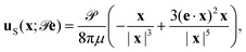 | (1) |
and the corresponding flow for a rotlet dipole of strength
χ is
2,29| | 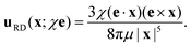 | (2) |
2.2 Geometry
Motivated by experimental results,22 we consider swimming bacteria confined within a cylinder of radius R = 20 µm and height D (which will vary), filled with a Newtonian fluid (water) of dynamic viscosity μ. All results will be presented in dimensionless variables (see Section 3). A population of N swimmers (where N will be varied) is constrained to a plane at a height h = 0.5 µm (approximately half the width of an E. coli cell body) above the bottom boundary, while a fixed number, n = 52, are constrained to a plane the same distance h below the top boundary, as illustrated in Fig. 1. This two-dimensional confinement captures the experimentally observed accumulation of the bacterial populations near their respective walls22 without requiring more computationally expensive fully three-dimensional simulations. We investigate the motion of the n swimmers near the top boundary (referred to below as “top swimmers”) under the influence of flows generated by the N swimmers near the bottom boundary (“bottom swimmers”) and their hydrodynamic images. This modelling choice assumes implicitly that the top population is smaller than the bottom population.
2.3 Swimming kinematics
Each swimmer is prescribed an intrinsic swimming speed U = 20 µm s−1.30 The bottom swimmers have their initial positions drawn from a uniform distribution over the disc at height h = 0.5 µm above the bottom boundary, and swim in the CW direction (as viewed from above) with speed U along concentric circles (see sketch Fig. 1). Each top swimmer is prescribed, in addition this intrinsic swimming speed U, an intrinsic angular velocity Ωẑ, so that a single top swimmer (in the absence of boundaries or flows from other swimmers) swims in its horizontal plane with a prescribed radius of curvature of RROC = 15 µm, consistent with experimental measurements.8–10 Here ẑ is the vertically upwards unit vector and Ω > 0 so that each top swimmer swims CCW with respect to the vertical (i.e. CW with respect to the normal pointing into the fluid).
2.4 Flows and steric effects on top swimmers
Each top swimmer experiences flows from the bottom swimmers and their images; the stresslet and rotlet dipole flows created by each bottom swimmer are modified due to the presence of the bottom boundary using the method of hydrodynamic images, whereby an appropriate combination of flow singularities is placed on the other side of the bottom surface such that the no-slip boundary condition is satisfied exactly on the bottom surface.29,31,32 By linearly superposing the flows from the singularities of each bottom swimmer, we are implicitly working in the framework of a dilute suspension of swimmers. It should also be noted that these approximate flows, however, do not satisfy the no-slip boundary conditions on the top wall. Nevertheless, this image-based representation provides a fundamental starting point for capturing the dominant hydrodynamic interactions experienced by the top population due to the bottom swimmers, and serves as a tractable approximation for studying their collective dynamics in the fully coupled system.
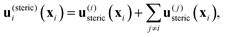
Each top swimmer interacts hydrodynamically and sterically with each other and with the top and lateral walls. In addition, we approximately account for hydrodynamic interactions between the top swimmer and the lateral circular boundary by placing image singularities outside the cylinder such that the superposition of the original singularities and the lateral wall images satisfy the no-slip boundary condition on the nearest tangent plane. These lateral wall hydrodynamic interactions for the top swimmers are essential to model correctly the wall-induced reorientation23 of the top swimmers parallel to the lateral wall, which in turn is required to reproduce a bacterial vortex. We neglect interactions between the top swimmers and the bottom boundary since they are much weaker than the top swimmer-top wall interactions. Steric interactions between swimmers are accounted for by soft repulsions in the form of velocities scaling as 1/r4, and steric interactions between swimmers and the circular boundary by 1/r6 repulsive velocities (where r indicates the swimmer–swimmer distance or the swimmer–wall distance).
The ith top swimmer, at a position xi, thus experiences a flow
| | | ui(xi) = u(steric)i(xi) + u(hydro)i(xi), | (3) |
where
| |  | (4) |
the sum of the steric interaction
u(i)steric(
xi) with the lateral wall and the steric interactions
u(j)steric(
xi) with the other top swimmers, and
| | 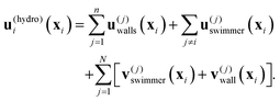 | (5) |
Here,
u(j)swimmer(
xi) is the flow experienced by the
ith top swimmer from the original flow singularities of the
jth top swimmer, given explicitly by
| | | u(j)swimmer(xi) = uS(xij;ej) + uRD(xij;χej), | (6) |
where
xij =
xi −
xj, and
ej is the orientation of the
jth swimmer.
u(j)walls(
xi) is the hydrodynamic images of each top swimmer with the top and lateral walls. The remaining terms
v(j)swimmer(
xi) +
v(j)wall(
xi) are flows from the bottom swimmers and their bottom wall images.
2.5 Time evolution of top swimmer positions and orientations
Confinement in the plane h = 0.5 µm below the top surface is implemented simply by setting the vertical component of any flow each top swimmer experiences to zero and initialising swimmers with their orientation vectors in the plane. The position of the ith swimmer is then evolved by numerically integrating| |  | (7) |
where ei is its orientation and no Einstein summation is implied in the second term on the right-hand side, and the (H) subscript denotes the planar projection of the flow velocity. The orientation is evolved according to (the planar projection of) Jeffery's equation33 for the motion of an ellipsoidal particle with the intrinsic rotational velocity Ωẑ common to all top swimmers,| | 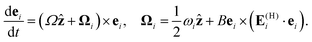 | (8) |
Here ωi is the z-component of the vorticity vector associated with u(hydro)i (see eqn (5));  , with Epq being the (p,q) component of the strain-rate tensor associated with u(hydro)i; and the shape factor B = (γ2 − 1)/(γ2 + 1), where γ is the aspect ratio of the ellipsoid.33 We approximate the flagellated bacterium as an ellipsoid of aspect ratio γ = 10, to model the combination of cell body and flagellar filaments.
2.6 Measure of global rotational direction
In each simulation, n = 52 top swimmers with random orientations are initially placed on a square grid. The proportion Φ of top swimmers in CCW motion (as viewed from the top) is measured at each time step. More precisely, a swimmer with instantaneous velocity ẋi := dxi/dt is defined to be in CCW motion if ẋi·![[small straight theta, Greek, circumflex]](https://www.rsc.org/images/entities/b_i_char_e12d.gif) > 0, where is the azimuthal basis vector in polar coordinates; the swimmer is otherwise in CW motion.
> 0, where is the azimuthal basis vector in polar coordinates; the swimmer is otherwise in CW motion.
The average value 〈Φ〉 over the time interval 15 s ≤ t < 30 s as well as the corresponding standard variation are recorded. We only consider values of Φ after t = 15 s in order to give ample time for the system to reach a dynamical steady state. A value of 〈Φ〉 close to 1 indicates that most swimmers are moving CCW, i.e. a CCW bacterial vortex, whereas 〈Φ〉 ≈ 0 corresponds to a CW bacterial vortex.
3 Rotation reversal of chiral bacterial vortices for sufficiently strong hydrodynamic interactions
We numerically investigate the behaviour of our model for different values of the height D and of the stresslet strength α and rotlet dipole strength β of the swimmers relative to the E. coli values = 2.19 µm pN and χ = 1.27 µm2 pN respectively. For each set of chosen parameters, we increase the number N of bottom swimmers and display plots of 〈Φ〉 against N in Fig. 2. The symbols indicate the average values of 〈Φ〉 obtained from each simulation, with the error bars indicating the standard deviation over the 15-second interval over which Φ is averaged. The curves, displayed for ease of visualisation, are rescaled and shifted tanh curves fitted to the data points: specifically each curve is generated by fitting the equation 〈Φ〉 = A0 + (A1 − A0){tanh[(N − N0)/δ] + 1}/2 to the data points (N, 〈Φ〉) obtained from the simulations, with A0, A1, δ and N0 as fitting parameters.
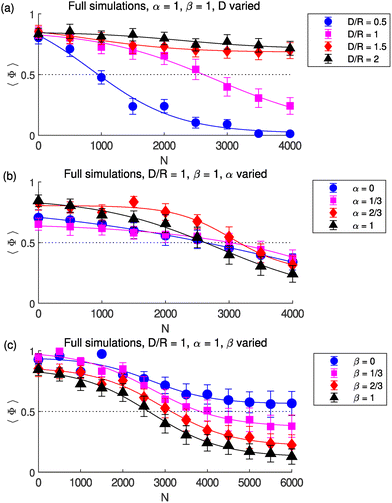 |
| | Fig. 2 Numerical simulations showing rotation reversal. Time-averaged proportion of top swimmers in CCW motion 〈Φ〉 against number N of bottom swimmers obtained from simulations with (a) α = β = 1 fixed and cylinder height D varied (b) D/R = β = 1 fixed and stresslet strength α varied (c) D/R = α = 1 fixed and rotlet dipole strength β varied. Error bars show the standard deviation over the 15 s window over which Φ is averaged. Curves are rescaled and shifted tanh curves fitted to the data points indicated by the symbols. Dotted line is at 〈Φ〉 = 0.5, indicating equal instances of CW motion and CCW motion. | |
3.1 Reversal of rotation direction as N is increased
As seen in Fig. 2, for all parameter values, 〈Φ〉 is close to 1 for N = 0 bottom swimmers, indicating a CCW vortex. The top swimmers near the lateral wall are attracted to it, and the majority move CCW along it due to the intrinsic angular velocity of each swimmer. However, a few cells swim CW depending on the angle of approach to the wall; this CW motion is short-lived, however, since these swimmers escape the wall due to interactions with other cells and eventually return to the bulk, where again the motion is more chaotic but dominantly CCW due to the intrinsic CW angular velocity (see Video S1).
Now consider the case α = β = D/R = 1 (the magenta curve in Fig. 2a). As the number of bottom swimmers is increased, 〈Φ〉 decreases and we observe a transition from global CCW motion (〈Φ〉 ≈ 1) at N = 0 to global CW motion at larger N. The flows created by the bottom swimmers, once strong enough, reverse the rotational direction of the population of top swimmers; at N = 2500 the top swimmers exhibit only a slight CCW global motion (see Video S2) while at N = 4000 the global rotation is clearly CW (see Video S3). This result qualitatively reproduces the reversal of the rotational direction of the smaller bacterial vortex seen in experiments.22 We also observe that at larger N the top swimmers are distributed closer to the centre (compare Videos S2 and S3 to Video S1).
3.2 Earlier rotation reversal for shallow chambers
For a smaller value of D/R = 0.5, i.e. for a shallower chamber, a smaller value of N is needed to drive this transition (Fig. 2a, blue curve). This is due to the top swimmers experiencing stronger flows at a closer distance to the bottom swimmers; equivalently, for the same value of N, the CW motion of the top swimmers is more prominent for D/R = 0.5 than for D/R = 1 (see Video S4). Conversely, for D/R = 1.5 and D/R = 2 (Fig. 2a, red and black curves respectively) the top swimmers experience much weaker flows from the bottom swimmers and although 〈Φ〉 does decrease with increasing N, the bottom swimmers' flows at these distances are not strong enough to reverse the top population's rotation direction even at N = 4000; see Video S5. We observe therefore a dramatic dependence of the top population's global rotation on D, consistent with the experimental observation that there is no reversal of rotational direction in sufficiently deep cylindrical microwells.22 These results are consistent with the rotation transition governed by hydrodynamic interactions.
3.3 Stresslet flows do not govern the rotation reversal
We next numerically vary the strengths of the dimensionless stresslet (α) and rotlet dipole (β) in order to elucidate the role each singularity plays in this CCW–CW transition. We first consider here variation of the stresslet strength and plot in Fig. 2b the transition curves for 〈Φ〉 for different values of α. Although the precise details of these curves vary with α due to a complex interplay of hydrodynamic interactions between the swimmers and the lateral wall, the CW–CCW transition is seen to occur at roughly the same value of N for all values of α, indicating that the stresslet flows do not provide the azimuthal flows driving the transition. We do observe that the top swimmers swim closer to the centre of the disc as α and N are increased, indicating that the stresslets create radially inwards flows. This effect however would be less noticeable in denser suspensions of bacteria since only a finite number of bacteria can occupy the area near the centre due to steric interactions. In Video S6 we show that the top swimmers, at sufficiently large N, indeed form a CW vortex without stresslets, and that without the stresslet flows from the bottom they are not pushed together towards the centre.
3.4 Rotation reversal is controlled by the rotlet dipoles
We observe instead that it is indeed the rotlet dipole flows which drive the CCW–CW transition. We show in Fig. 2c that, as the rotlet dipole strength β is decreased from β = 1 (black) to β = 2/3 (red) and β = 1/3 (magenta), the CCW–CW transition occurs at larger and larger N. Equivalently, for a fixed value of N, 〈Φ〉 is larger (i.e. the motion is less CW) for smaller β. For β = 0 i.e. non-chiral swimmers, 〈Φ〉 asymptotes at 0.5 for large N and there is no transition at all.
These top swimmers move CCW along the wall at smaller N because of their intrinsic angular velocity, but at larger N are clumped together near the centre and without the influence from the lateral wall are unable to exhibit global rotational motion (see Video S7). These results show clearly that hydrodynamic interactions govern the reversal of rotational direction observed experimentally, and that it is the rotlet dipoles, and therefore the chirality of the hydrodynamic flows, which drive the CCW–CW transitions.
4 Theoretical analysis
Our numerical simulations have revealed that purely through hydrodynamic interactions, a rotation reversal occurs for chiral bacterial vortices if these interactions are sufficiently strong. We now propose a theoretical analysis in order to rationalise these results.
4.1 Leading-order flows experienced by top swimmers
4.1.1 Numerical flows.
The first piece of our theoretical analysis consists of deriving an approximation for the swimming-induced flows. We can use our simulations to compute the horizontal components of the flow fields in the plane of the top swimmers due to the bottom swimmers. In the case N = 1000, we plot in Fig. 3 the contributions from the rotlet dipoles (Fig. 3a), the contributions from the stresslets (Fig. 3b), and the combined flow (Fig. 3c). These flow fields are consistent with our results in the previous section and we now proceed to calculate theoretical models for these flow fields.
 |
| | Fig. 3 Swimmer flows. Map of flow field in the plane occupied by the top swimmers created by N = 1000 bottom swimmers, as computed numerically (a)–(c) and theoretically (d)–(f) for swimmers with only rotlet dipoles (α = 0, β = 1; panels (a) and (d)), only stresslets (α = 1, β = 0; panels (b) and (e)), and both rotlet dipoles and stresslets (α = β = 1; panels (c) and (f)). The dotted circle in each plot indicates the cylinder wall. | |
4.1.2 Rotlet-dipoles flows.
Using Cartesian coordinates centred at the centre of the bottom wall and with the positive z direction pointing upwards, the bottom wall is defined by the disc a(a, s) = (a![[thin space (1/6-em)]](https://www.rsc.org/images/entities/char_2009.gif) coss, asins, 0) with 0 < a ≤ R, 0 < s ≤ 2π. In the limit of large N, the flows created by the N bottom swimmers is approximately given by the flow created by a continuous distribution of flow singularities in the disc a(a, s) + h with 0 < a ≤ R, 0 < s ≤ 2π with a uniform number density ρ := N/πR2, where h = hẑ, and with the flow singularity at a(a, s) oriented in the direction e(s) = (sins, −coss, 0). Their hydrodynamic images are located in the disc a(a, s) − h with 0 < a ≤ R, 0 < s ≤ 2π. Note that in the large-N continuum limit the distribution of bottom swimmer singularities, and therefore the flows they create, are time-invariant, and in particular are independent of the swimming speed U of the bottom swimmers and of whether they swim CW or CCW.
coss, asins, 0) with 0 < a ≤ R, 0 < s ≤ 2π. In the limit of large N, the flows created by the N bottom swimmers is approximately given by the flow created by a continuous distribution of flow singularities in the disc a(a, s) + h with 0 < a ≤ R, 0 < s ≤ 2π with a uniform number density ρ := N/πR2, where h = hẑ, and with the flow singularity at a(a, s) oriented in the direction e(s) = (sins, −coss, 0). Their hydrodynamic images are located in the disc a(a, s) − h with 0 < a ≤ R, 0 < s ≤ 2π. Note that in the large-N continuum limit the distribution of bottom swimmer singularities, and therefore the flows they create, are time-invariant, and in particular are independent of the swimming speed U of the bottom swimmers and of whether they swim CW or CCW.
We first calculate the flows due to the rotlet dipoles and their bottom wall images. The flow field at a position x = (x, y, z) due to the rotlet dipole at a(a, s) + h and its image is given by
| |  | (9) |
where we write
r =
x −
a,
e⊥ = (cos
t, sin
t, 0). Here the final four terms are the image singularities of the rotlet dipole, placed at an image point on the other side of the wall, with
RD,
Q, and
GQ denoting rotlet dipole, source quadrupole, and stokeslet quadrupole respectively; this image system is derived in ref.
29.
We consider the far field limit |x| ≫ a, h, so
| |  | (10) |
where
r = |
r|. Taylor expanding the first two terms in
eqn (9) gives
| |  | (11) |
The third term is also of the same order,
| | 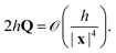 | (12) |
The leading-order contribution is from the final two terms, i.e.
| | 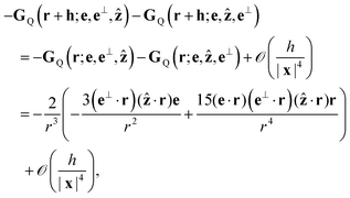 | (13) |
where several terms in the expressions for
GQ have vanished by orthogonality of {
e,
e⊥,
ẑ} or because they are antisymmetric with respect to interchanging
e⊥ and
ẑ. Note that this is invariant with respect to the reversal of the rotational direction of the bottom swimmers (
e,
e⊥) ↦ −(
e,
e⊥), consistent with the front-back symmetry of the rotlet dipole. An analogous statement holds for the stresslet.
We next expand vectors into their components and integrate with respect to s to obtain
| |  | (14) |
| |  | (15) |
Putting
eqn (10)–(15) together and integrating with respect to
a yields the final result for the leading order flow field in the far field of a disc of azimuthally oriented rotlet dipoles above a no-slip boundary,
| |  | (16) |
which is a rotlet dipole of strength −
χẑ. In the plane of the top swimmers (
z > 0) this flow acts in the CW direction as we would expect; this theoretical prediction is shown in
Fig. 3d. Note that this leading order flow is independent of
h, so although a more detailed consideration of wall–swimmer interactions may motivate a different value of
h,
34,35 the precise modelling choice would not impact our main results. It is worth noting, as may be shown by a similar calculation, that the leading order flow field due to the same disc of rotlet dipoles in the absence of a wall is a rotlet dipole of strength −
χẑ/2, so the presence of the bottom wall amplifies the CW flows.
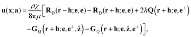
4.1.3 Stresslet flows.
We may carry out similar calculations for the stresslets. Specifically, we derive the horizontal component of the (leading-order) flow field at a position x = (x, y, z) produced by a distribution of azimuthally oriented stresslets, each of strength , distributed with uniform number density ρ = N/πR2 on the horizontal disc of radius R centred at (0, 0, h), together with their images due to a no-slip boundary at z = 0. This flow field due to the stresslet at a(a, s) + h and its image is given by| | | u(x;a) = ρ[GD(r − h;e,e) − GD(r + h;e,e) + 2hGQ(r + h;e,e,ẑ) − 2h2Q(r + h;e,e)], | (17) |
where GD, GQ, and Q are a stokeslet dipole, stokeslet quadrupole, and a source quadrupole, respectively.29
As above, we consider the far field limit |x| ≫ a, h and neglect terms linear in a. In contrast to the rotlet dipole calculations, however, the lowest order terms are linear in h. The dominant contributions are from the first three terms of eqn (17) since the fourth term is quadratic in h. In what follows we use a (H) superscript to denote horizontal components. A Taylor expansion of the first two terms yields
| |  | (18) |
The stokeslet quadrupole term may be evaluated to be
| |  | (19) |
We therefore obtain the flow field due at x due to a single stresslet and its image as
| |  | (20) |
Noting that
h·
r =
hz and

and integrating over the disc, we get our final result for the horizontal component of the flow field at
x induced by the disc of stresslets,
| |  | (21) |
This is radially inwards provided x2 + y2 < 3z2/2; for D/R = 1,  so this flow is always radially inwards at the top swimmers' positions. This theoretical flow field is plotted in Fig. 3e.
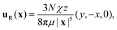
The far-field approximation of the horizontal component of the flow experienced by the top swimmers at x = (x, y, z) due to the disc of N bottom swimmers is therefore given by the sum
| | 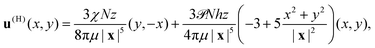 | (22) |
and this flow field is illustrated in
Fig. 3f.
Note that while our leading order expressions overestimate the flow speeds especially towards the centre since this is where our far field assumption |x| ≫ a holds least well, our theoretical flows exhibit the right qualitative behaviour (compare Fig. 3a–c with Fig. 3d–f) and thus capture the main physical ingredients.
Note that, at this order in a, the flow is independent of the radial distribution of bottom swimmers and depends only on their total number N. Future work could explore, either numerically or theoretically using higher-order corrections in a, the impact of non-uniform bottom distributions. Although here we treat the bottom population as unaffected by the top population's flows due to its smaller size, such an approach may provide a first step toward relaxing this assumption.
4.2 Simulations of top swimmers subject to theoretical flows
In order to demonstrate that the theoretical flows are able to explain the CCW–CW transitions, we next carry out simulations of the top swimmers subject to this theoretical flow i.e. with the numerically computed flows  from the N bottom swimmers and their images replaced with eqn (22). The results are shown in Fig. 4 and, strikingly, recover the same behaviour as the full simulations shown in Fig. 2. The CCW–CW transition occurs at larger N as D increases (Fig. 4a); this is due to the fast decay D−4 of the rotlet dipole flows in eqn (22). Note that we have omitted results for D/R = 0.5 because our theoretical calculations are not valid for this value of D as the far field assumption |x| ≫ a does not hold. We further recover theoretically, as we saw in the full simulations, that the stresslet strength does not have a significant effect on the CCW–CW transition (Fig. 4b), and that the transition occurs at larger N as the rotlet dipole strength is decreased, with no transition at all (〈Φ〉 asymptoting at 0.5) where the rotlet dipoles are gone (β = 0, Fig. 4c). By taking the continuum and far-field limits of the bottom population, we derived analytical approximations for the flow field from the bottom swimmers, and subjecting a top swimmer population to these theoretical flows, we therefore successfully reproduced the CCW–CW transition and its dependence on the cylinder height and the different flow singularity components.
 |
| | Fig. 4 Rotation reversal from theory. Plots of time-averaged proportion 〈Φ〉 of top swimmers in CCW motion against number N of bottom swimmers obtained from the theoretical approximation of the flows due to the bottom swimmers, with (a) α = β = 1 fixed and cylinder height D varied (b) D/R = β = 1 fixed and stresslet strength α varied (c) D/R = α = 1 fixed and rotlet dipole strength β varied. Error bars show the standard deviation over the 15-s window over which Φ is averaged. Curves are rescaled tanh curves fitted to the data points indicated by the symbols. Dotted line is at 〈Φ〉 = 0.5, indicating equal instances of CW motion and CCW motion. Dashed lines indicate theoretical estimates of critical bottom population size (eqn (29)) at which the CCW–CW transition occurs. These results are to be compared with the full simulations shown in Fig. 2. | |
4.3 Theory for swimmer trajectory
We may further carry out an analytical calculation for the simpler case of a single top swimmer, in order to analytically predict the CCW–CW transition threshold as a function of the parameters of the system. The governing equations for the position x and orientation p of a single swimmer at the top, neglecting its interactions with the top and lateral walls, are| | 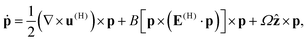 | (24) |
where U and Ω are its intrinsic translational and angular velocities; u(H) (as given in eqn (22)), is the planar projection of the flow due to the bottom swimmers; and  is the planar projection of the strain-rate tensor associated with u(H). These projections ensure that the equations are 2D and that the swimmer direction and orientations remain in the plane given in-plane initial conditions. The result in eqn (24) is (the 2D projection of) the classical Jeffery's equation describing how an elongated particle reorients in a flow (this is in fact eqn (8) for a single top swimmer). The first term is the reorientation due to the fluid velocity, and the second term describes how an elongated particle interacts with the strain rate and aligns with the flow; B is the shape factor governing this strain rate interaction. We work in the far-field limit x, y, h ≪ r, so to leading order we may write |x| ≈ z ≈ D and neglect the (x2 + y2)/|x|2 term in the stresslet flow field, so eqn (22) then linearises to
| | 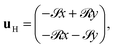 | (25) |
where ![[scr S, script letter S]](https://www.rsc.org/images/entities/char_e532.gif) = 9Nh/4πμD4 and
= 9Nh/4πμD4 and ![[scr R, script letter R]](https://www.rsc.org/images/entities/char_e531.gif) = 3χN/8πμD4. We then have E = −I so the shape-dependent terms in Jeffery's equation vanish at this order. Writing p = (cosϕ, sinϕ), the governing equations simplify to
= 3χN/8πμD4. We then have E = −I so the shape-dependent terms in Jeffery's equation vanish at this order. Writing p = (cosϕ, sinϕ), the governing equations simplify to| | 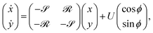 | (26) |
| | ![[small phi, Greek, dot above]](https://www.rsc.org/images/entities/i_char_e0a3.gif) = (Ω − )t. = (Ω − )t. | (27) |
The ϕ equation integrates easily to ϕ = ϕ0 + (Ω − )t. The matrix in the (x, y) equation has eigenvalues λ± = − ± i, so the complementary function decays exponentially. The particular integral is then a limit cycle of the system, and may be calculated to be
| | 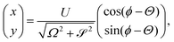 | (28) |
where tan
Θ =
Ω/
. Hence, we theoretically predict that trajectories eventually converge to a circle of radius
. This limiting radius
![[R with combining tilde]](https://www.rsc.org/images/entities/i_char_0052_0303.gif)
decreases as the stresslet strength increases as we would expect from the radially inwards flow created a disc of stresslets, and from the results of our numerical simulations.
Crucial, whether the trajectories are CW or CCW depend on the sign of : indeed, the trajectories are CCW for < Ω and transition to CW when > Ω. Hence we predict the critical value of N at which the transition occurs to be
| |  | (29) |
This theoretical result is plotted as dashed vertical lines in
Fig. 4 for comparison with the critical bottom population size at which the transition occurs for a population of top swimmers subject to the far-field theoretical flows, and we see remarkable agreement for the base case
D/
R =
α =
β = 1. The larger discrepancies for other parameter values are unsurprising given the simplifications made to reach this result (in particular the assumption of a single top swimmer). Regardless, this expression is in qualitative agreement with our numerical results, and an examination of the parametric dependence gives us physical insight. The scaling
Nc ∼
D4 is consistent with how the CCW–CW transition occurs at dramatically larger
N as
D is increased (
Fig. 2a), while the
Nc ∼ 1/
χ dependence is consistent with the plots with the rotlet strength varied (
Fig. 2c). Note also that the critical
Nc does not depend on the stresslet (consistent with
Fig. 2b). The single expression in
eqn (29) thus encapsulates all our findings, revealing how the top bacterial vortex reverses its global rotation due to rapidly decaying flows created by the chirality of bottom swimmers.
5 Conclusion
Using a model based on flow singularities, we studied computationally the reversal of the rotational direction of a bacterial vortex near a flat surface of a cylindrical geometry due to the presence of a larger bacterial vortex near the opposite flat surface. We carried out simulations for a range of values of cylinder height and flow singularity strengths, comprehensively exploring how the rotation reversal depends on these parameters. We further carried out theoretical calculations in the far field and continuum limits of the flows produced by a disc of azimuthally aligned swimmers near a no-slip boundary, and performed simulations of top swimmers subject to these theoretical flows. We obtained results consistent with the full simulations, illustrating that the far-field flows are sufficient to induce rotation reversal. We then investigated analytically the simpler case of a single chiral swimmer advected and rotated by the flows from a bacterial vortex, and determined expressions for the eventual circular trajectory of the swimmer and for the critical size Nc of the bacterial vortex at which the trajectory of the swimmer transitions from CCW to CW motion.
These analytical results capture the essential physics driving the rotation reversals: the azimuthal flows from the rotlet dipoles. The stresslets create radially inward flows, which manifest as a smaller radius of the eventual swimmer trajectory as stresslet strength is increased, but are largely inconsequential for the global rotational motion. These flows decay rapidly away from the bottom population, explaining the dramatic dependence of the critical bottom population size at which rotation reversal occurs.
Although our far-field model neglects details of near-field interactions, flow singularities have been used in the past to successfully explain a number of hydrodynamic phenomena,6 and in particular a similar approach has been recently used to successfully rationalise the self-organisation of confined magnetotactic bacteria into convective plumes under the application of a magnetic field.25 In this work, we have used flow singularities to characterise the rotation reversal of bacterial vortices with similar success. Our model could be made more realistic by performing fully three-dimensional simulations in which accumulation of bacteria near the flat surfaces, which we have modelled by confining the swimmers to a plane, would naturally arise from hydrodynamic interactions of the stresslets with the walls. While this might be challenging since the exact solutions for point forces/torques (or their dipoles) in a closed cylinder are not known, an alternative approach would be to explore a similar system in a spherical geometry, for which these solutions are available.36 Our singularities-based treatment does not take into account near-field effects between interacting bacteria,37 possible lubrication effects for swimmers near surfaces, or direct fluid entrainment from the bottom population. Placing the two populations on more equal footing and allowing mutual flow interactions would yield a more physically faithful model. An alternative modelling approach would consist of a hydrodynamic theory treating the bacterial suspension as an effective continuum phase to characterise mesoscale flow behaviour.19,38,39 Despite the numerous idealisations, our minimal model captures the essential physics of the system and illustrates clearly that the intrinsic chirality of individual bacteria, captured by the rotlet dipole, cooperates at the population scale to drive the reversal of collective rotational motion. We also expect that similar methods may find broader applications at larger length scales, for example, in the context of circular mills of worms.40 The success of our model at rationalising the reversal of bacterial vortices, as well as its wider implications, highlight the value of flow singularities and far-field calculations as powerful tools for rationalising biophysical phenomena.
Conflicts of interest
There are no conflicts to declare.
Data availability
The data supporting this article have been included as part of the supplementary information (SI). Supplementary information: videos S1–S7 of simulations for the following parameters. Video S1: D/R = 1, α = 1, β = 1, N = 0. Video S2: D/R = 1, α = 1, β = 1, N = 2500. Video S3: D/R = 1, α = 1, β = 1, N = 4000. Video S4: D/R = 0.5, α = 1, β = 1, N = 4000. Video S5: D/R = 1.5, α = 1, β = 1, N = 4000. Video S6: D/R = 1, α = 0, β = 1, N = 4000. Video S7: D/R = 1, α = 1, β = 0, N = 4000. Supplementary information is available. See DOI: https://doi.org/10.1039/d5sm00889a.
Modelling code for this study has been uploaded onto the Zenodo repository https://doi.org/10.5281/zenodo.17988389.
Acknowledgements
We thank Sarah Waters and Raymond Goldstein for useful feedback on an earlier version of this work. This project has received funding from the European Research Council under the European Union's Horizon 2020 research and innovation program (Grant No. 682754 to E. L.), and the Cambridge Trust (scholarship to P. H. H.).
References
- C. Brennen and H. Winet, Annu. Rev. Fluid Mech., 1977, 9, 339–398 CrossRef.
-
E. Lauga, The Fluid Dynamics of Cell Motility, Cambridge University Press, 2020 Search PubMed.
-
H. C. Berg, E. coli in Motion, Springer, New York, NY, 2004 Search PubMed.
-
D. Bray, Cell movements: from molecules to motility, Garland Science, 2000 Search PubMed.
- A. Chwang and T. Y. Wu, Proc. R. Soc. London, Ser. B, 1971, 178, 327–346 CAS.
- E. Lauga and T. R. Powers, Rep. Prog. Phys., 2009, 72, 096601 CrossRef.
- Y. Hyon, Marcos, T. R. Powers, R. Stocker and H. C. Fu, J. Fluid Mech., 2012, 705, 58–76 CrossRef.
- E. Lauga, W. R. DiLuzio, G. M. Whitesides and H. A. Stone, Biophys. J., 2006, 90, 400–412 CrossRef CAS PubMed.
- P. D. Frymier, R. M. Ford, H. C. Berg and P. T. Cummings, Proc. Natl. Acad. Sci. U. S. A., 1995, 92, 6195–6199 CrossRef CAS.
- P. D. Frymier and R. M. Ford, AIChE J., 1997, 43, 1341–1347 CrossRef CAS.
- M. A. Vigeant and R. M. Ford, Appl. Environ. Microbiol., 1997, 63, 3474–3479 CrossRef CAS.
- W. R. Diluzio, L. Turner, M. Mayer, P. Garstecki, D. B. Weibel, H. C. Berg and G. M. Whitesides, Nature, 2005, 435, 1271–1274 CrossRef CAS.
- C. W. Wolgemuth, Biophys. J., 2008, 95, 1564–1574 CrossRef CAS PubMed.
- T. Ishikawa and T. J. Pedley, Phys. Rev. Lett., 2008, 100, 088103 CrossRef.
- D. Saintillan and M. J. Shelley, Phys. Rev. Lett., 2008, 100, 178103 CrossRef.
- J. P. Hernandez-Ortiz, C. G. Stoltz and M. D. Graham, Phys. Rev. Lett., 2005, 95, 204501 CrossRef.
- D. L. Koch and G. Subramanian, Annu. Rev. Fluid Mech., 2011, 43, 637–659 Search PubMed.
-
L. Cisneros, R. Cortez, C. Dombrowski, R. Goldstein and J. Kessler, Anim. Locomotion, 2010, pp. 99–115 Search PubMed.
- H. Wioland, F. G. Woodhouse, J. Dunkel, J. O. Kessler and R. E. Goldstein, Phys. Rev. Lett., 2013, 110, 268102 CrossRef.
- E. Lushi, H. Wioland and R. E. Goldstein, Proc. Natl. Acad. Sci. U. S. A., 2014, 111, 9733–9738 CrossRef CAS PubMed.
- D. Huang, Y. Du, H. Jiang and Z. Hou, Phys. Rev. E, 2021, 104, 034606 Search PubMed.
- K. Beppu, Z. Izri, T. Sato, Y. Yamanishi, Y. Sumino and Y. T. Maeda, Proc. Natl. Acad. Sci. U. S. A., 2021, 118, e2107461118 Search PubMed.
- A. P. Berke, L. Turner, H. C. Berg and E. Lauga, Phys. Rev. Lett., 2008, 101, 038102 Search PubMed.
- A. T. Chwang and T. Y.-T. Wu, J. Fluid Mech., 1975, 67, 787–815 CrossRef.
- A. Thery, L. Nagard, J.-C. Ono-dit Biot, C. Fradin, K. Dalnoki-Veress and E. Lauga, Sci. Rep., 2020, 10, 13578 CrossRef CAS.
- D. Lopez and E. Lauga, Phys. Fluids, 2014, 26, 071902 Search PubMed.
- J. Hu, M. Yang, G. Gompper and R. G. Winkler, Soft Matter, 2015, 11, 7867–7876 Search PubMed.
- K. Drescher, J. Dunkel, L. H. Cisneros, S. Ganguly and R. E. Goldstein, Proc. Natl. Acad. Sci. U. S. A., 2011, 108, 10940–10945 Search PubMed.
- S. E. Spagnolie and E. Lauga, J. Fluid Mech., 2012, 700, 105–147 Search PubMed.
- S. Chattopadhyay, R. Moldovan, C. Yeung and X. L. Wu, Proc. Natl. Acad. Sci. U. S. A., 2006, 103, 13712–13717 Search PubMed.
- J. R. Blake, Math. Proc. Cambridge Philos. Soc., 1971, 70, 303–310 CrossRef.
- J. R. Blake and A. T. Chwang, J. Eng. Math., 1974, 8, 23–29 CrossRef.
-
S. Kim and S. J. Karrila, Microhydrodynamics: Principles and Selected Applications, Dover, 1991 Search PubMed.
- H. Shum, E. A. Gaffney and D. J. Smith, Proc. R. Soc. London, Ser. A, 2010, 466, 1725–1748 Search PubMed.
- P. H. Htet, D. Das and E. Lauga, Phys. Rev. Res., 2024, 6, L032070 CrossRef CAS.
- A. Chamolly and E. Lauga, Phys. Rev. Fluids, 2020, 5, 074202 Search PubMed.
- B. Zhang, P. Leishangthem, Y. Ding and X. Xu, Proc. Natl. Acad. Sci. U. S. A., 2021, 118, e2100145118 Search PubMed.
- S. Heidenreich, J. Dunkel, S. H. L. Klapp and M. Bär, Phys. Rev. E, 2016, 94, 020601 Search PubMed.
- H. Reinken, S. H. L. Klapp, M. Bär and S. Heidenreich, Phys. Rev. E, 2018, 97, 022613 CrossRef CAS.
- G. T. Fortune, A. Worley, A. B. Sendova-Franks, N. R. Franks, K. C. Leptos, E. Lauga and R. E. Goldstein, J. Fluid Mech., 2021, 914, A20 CrossRef CAS.
Footnote |
| † Current address: Department of Mathematics, Kyoto University, Kyoto 606-8502, Japan. |
|
| This journal is © The Royal Society of Chemistry 2026 |
Click here to see how this site uses Cookies. View our privacy policy here. 
 Open Access Article
 This Open Access Article is licensed under a Creative Commons Attribution-Non Commercial 3.0 Unported Licence
 and
Eric
Lauga
and
Eric
Lauga


 , with Epq being the (p,q) component of the strain-rate tensor associated with u(hydro)i; and the shape factor B = (γ2 − 1)/(γ2 + 1), where γ is the aspect ratio of the ellipsoid.33 We approximate the flagellated bacterium as an ellipsoid of aspect ratio γ = 10, to model the combination of cell body and flagellar filaments.


 and integrating over the disc, we get our final result for the horizontal component of the flow field at x induced by the disc of stresslets,
 so this flow is always radially inwards at the top swimmers' positions. This theoretical flow field is plotted in Fig. 3e.
 from the N bottom swimmers and their images replaced with eqn (22). The results are shown in Fig. 4 and, strikingly, recover the same behaviour as the full simulations shown in Fig. 2. The CCW–CW transition occurs at larger N as D increases (Fig. 4a); this is due to the fast decay D−4 of the rotlet dipole flows in eqn (22). Note that we have omitted results for D/R = 0.5 because our theoretical calculations are not valid for this value of D as the far field assumption |x| ≫ a does not hold. We further recover theoretically, as we saw in the full simulations, that the stresslet strength does not have a significant effect on the CCW–CW transition (Fig. 4b), and that the transition occurs at larger N as the rotlet dipole strength is decreased, with no transition at all (〈Φ〉 asymptoting at 0.5) where the rotlet dipoles are gone (β = 0, Fig. 4c). By taking the continuum and far-field limits of the bottom population, we derived analytical approximations for the flow field from the bottom swimmers, and subjecting a top swimmer population to these theoretical flows, we therefore successfully reproduced the CCW–CW transition and its dependence on the cylinder height and the different flow singularity components.


 is the planar projection of the strain-rate tensor associated with u(H). These projections ensure that the equations are 2D and that the swimmer direction and orientations remain in the plane given in-plane initial conditions. The result in eqn (24) is (the 2D projection of) the classical Jeffery's equation describing how an elongated particle reorients in a flow (this is in fact eqn (8) for a single top swimmer). The first term is the reorientation due to the fluid velocity, and the second term describes how an elongated particle interacts with the strain rate and aligns with the flow; B is the shape factor governing this strain rate interaction. We work in the far-field limit x, y, h ≪ r, so to leading order we may write |x| ≈ z ≈ D and neglect the (x2 + y2)/|x|2 term in the stresslet flow field, so eqn (22) then linearises to


 . This limiting radius