Multi-technique computational assessment of fluoride uptake in enamel using PIGE, NEXAFS, and Raman spectroscopy

Abstract

The uptake of fluoride in the enamel matrix is an effective strategy to prevent demineralization and caries formation. In this study a comprehensive methodology is developed to evaluate and understand the uptake of fluoride in human enamel. Twenty-six healthy anterior teeth were sectioned in half; one half remained untreated, while the other was treated with 50 mg mL⁻¹ NaF (equivalent to 22.6 mg of fluoride) through three 1-minute applications over a 12-day period, following the manufacturer's guidelines. Fluoride uptake was quantified with particle-induced gamma-ray emission (PIGE), revealing an average increase of 160% in treated samples. The formation of calcium fluoride (CaF₂) and fluorapatite-like structures was confirmed through near edge X-ray absorption fine structure (NEXAFS) analysis. Due to the absence of reference spectra for hydroxyapatite, fluorapatite, and calcium fluoride, finite difference method near edge structure (FDMNES) simulations were employed to computationally model the fluorine K-edge and the Ca L-edge spectra. Density functional theory (DFT) and time-dependent DFT (TDDFT) approaches were applied to enhance spectral accuracy, enabling a refined comparison with experimental data. To establish a rapid and laboratory-based screening technique, Raman microscopy was used to analyze fluoride-treated and untreated samples. Spectral data were evaluated using both full-spectrum analysis and specific spectral features, including band intensity, full-width at half maximum (FWHM) of Raman peaks, and phosphate symmetric stretching depolarization ratios. Furthermore, machine learning algorithms were applied to classify treated and untreated enamel samples. The random forest classifier demonstrated strong predictive performance, successfully distinguishing fluoride-treated samples. This methodological approach provides an effective framework for analyzing fluoride uptake in enamel, potentially guiding future preventive dentistry strategies.

---

1. Introduction

Based on epidemiological evidence, it is estimated that around 2.4 billion people suffer from dental caries, a chronic infectious disease that results in the demineralization of human tooth enamel.¹ This destruction of the calcified tissues of the tooth occurs through acidic attack resulting from bacteriological activity (mainly Streptococcus mutans),² which metabolize carbohydrates and produce acids as by-products, thus leading to a decrease in pH in the oral cavity.

Another leading cause of enamel deconstruction is tooth erosion beginning with the demineralization of the surface layers of enamel and ultimately progressing to significant loss of tooth structure. The acids responsible for dental erosion can be intrinsic or extrinsic.³ While extrinsic factors are related to eating habits (use of carbohydrates) and lifestyle, intrinsic factors can be caused by systemic diseases.⁴ In this context, direct exposure to acids in the oral cavity promotes the demineralization of hydroxyapatite (Ca₅(PO₄)₃(OH) − HAp), due to the sub saturation of minerals in relation to the surrounding microenvironment.^4,5

Several studies^6,7 have demonstrated that the application of topical fluoride agents in enamel could prevent the formation of dental caries by strengthening the tooth matrix.

The replacement of hydroxyl groups with smaller fluoride ions should result in a more stable apatitic structure. If the OH⁻ ion in the pure hydroxyapatite is completely replaced by a fluoride ion (F⁻) the resulting mineral is fluorapatite [Ca₅(PO₄)₃F].⁸ The lower solubility and greater mechanical strength of FAp compared to HAp increases the mineral's resistance to demineralization, thus reducing the development and prevalence of caries.^9,10 In a situation where the enamel has been demineralized, its repair is possible by re-embedding the lost ions. An increase in the pH of saliva is a necessary condition for this process to take place, so in the presence of fluoride ions, remineralization occurs faster and at a lower pH and the restored enamel becomes stronger.¹⁰

However, apart from the iso–ionic exchange of fluorine for hydroxyl, there are other forms of fluoride ion reactivity with apatite: there can be crystal growth of fluorapatite from supersaturated solutions or the apatite dissolution and formation of CaF₂-like crystals, and alternative loosely bound forms of fluoride on the enamel crystallite surface.¹¹

In general, regardless of the efficacy of fluoride in in vitro studies, clinical results are mostly below expectations and are mainly due to the lack of reliable methods for assessing the formation of FAp in enamel, which would make it possible to select the best candidate materials for clinical tests and the development of efficient tooth fluoridation materials.¹²

Since the condition of human teeth is determined by changes occurring in the phase composition of the tissue at the micro and nano level, the use of spectroscopic methods of molecular identification is the most promising and sensitive tool to precisely assess such changes in the dental enamel.¹³ Raman spectroscopy is most often used for the examination of tooth samples to evaluate the demineralization effect of fluorinated pharmaceutical products, such as whitening gels,^14,15 protective varnishes^16,17 and gustative stimulants¹⁸ mainly by gauging the depolarization ratio of the symmetric stretching of phosphate. Although the efficacy of the protective effect against demineralization was proven in these studies, there is a lack of evidence of the factual formation of FAp, perhaps due to the low-resolution of the used system, or limited availability of datasets.

In this study we compare the Raman profiles of dental enamel with and without the application of topical NaF, with the ambition of identifying the formation of novel phases in the enamel composition using this non-destructive technique. For this purpose, we used supervised and unsupervised machine learning (ML) algorithms to further evaluate and classify our samples.

Raman spectroscopy generates a large multivariate dataset that consists of a series of data points representing the intensity of Raman scattering at specific frequencies. Advances in artificial intelligence (AI), particularly in machine learning (ML) algorithms have become effective tools for analyzing complex Raman datasets, by optimizing computational time and preprocessing of spectral data¹⁹ and identifying patterns in the dataset as well as performing classification in a more efficient way.^20,21 These algorithms can identify and classify different molecular species, phases, or materials present in a sample based on the spectral data.²⁰

The validation of the uptake of fluorine in the enamel was performed using the particle induced gamma-ray emission (PIGE) technique, whereas the evaluation of alterations in the electronic structure of some enamel samples was performed using near edge X-ray absorption fine structure (NEXAFS). PIGE and NEXAFS are very sensitive techniques that require the use of large facilities, such as particle accelerators for proton beams and synchrotron radiation, respectively. While PIGE has been used profusely to quantify low-Z elements like fluorine in hydroxyapatite matrices,^14,18,22,23 the use of NEXAFS has been seldomly exploited^24,25 so the characterization of the structure of hydroxyapatite-based samples has been limited.

In this study, samples of human teeth enamel were evaluated via polarized Raman microscopy, PIGE and NEXAFS in order to search for conclusive evidence of the formation of fluorapatite in the enamel and to establish a methodology for this evaluation using a low maintenance laboratory-based technique, with screening capabilities, such as Raman microscopy.

2. Materials and methods

2.1. Sample description and preparation

Twenty-six anterior healthy teeth, extracted for periodontal or orthodontic reasons and preserved in a 0.5% (w/w) chloramine solution for no longer than 6 months, from the LIBPhys-FMDUL tooth bank, were selected. The samples were selected by experts and the exclusion criterion was the presence of lesions. Hydroxyapatite is an anisotropic material, thus, signal intensity might be affected by the crystallographic orientation.^26,27 This way, and in order to minimize the effects of crystallographic orientation of the samples, specimens were obtained only from molar teeth with a precision diamond saw (Buehler Isomet 1000, USA). Because human teeth in the biobank are anonymized and we are not aware of previous history of fluoride treatments, paired specimens were obtained from each tooth, one for the control group (C) and another for the treatment (with NaF paste) group (T).

Specimens from the T group were treated with Colgate® Duraphat®, containing 50 mg ml⁻¹ of NaF, equivalent to 22.6 mg of fluoride. The treatment consisted of 3 applications, 1 minute each, over a 12-day period. After each application, the specimens were brushed under running water using a soft toothbrush in order to remove traces of the paste, and were stored in vials at room temperature with damp cotton to prevent dehydration.

No further preparation was required for the characterization of the samples using PIGE, Raman or NEXAFS.

2.2. Particle induced gamma ray emission (PIGE)

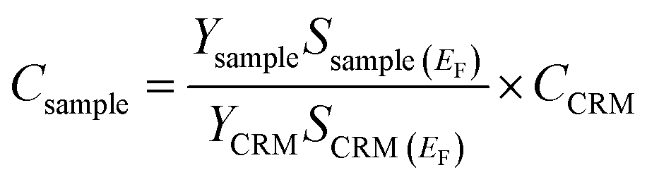
The prepared samples were evaluated using PIGE in order to gauge the uptake of fluorine. The experimental work for PIGE was carried out at the Centro Nacional de Aceleradores (CNA) in the Seville 3 MV Tandem accelerator, using 3800 keV protons. The current used was approximately 2 nA, and the total charge collected was 0.5, 1 or 1.5 μC per measurement. Before entering the reaction chamber, the beam passes through a collimator which defines a beam spot of around 0.5 mm on the sample, allowing, in this case, three different spots per mandible to be analyzed. The fluorine gamma-rays from the ¹⁹F(p,p′γ)¹⁹F nuclear reaction, at 197 keV, and the sodium gamma-rays from the ²³Na(p,p′γ)²³Na, at 440 keV, were detected by a Ge(HP) (hyper pure germanium) semiconductor detector.

Peak intensities were obtained using the MatLab® (MathWorks, USA) function trapz (trapezoidal numerical integration) that computes the approximate integral via the trapezoidal method. Quantification was performed using the certified reference material (CRM) (Bone Ash – NIST 1400) according to:²⁸

where C_sample and C_CRM, are the element concentrations in the sample and CRM, respectively; Y_sample and Y_CRM, are element gamma-ray yields (net peak areas) for the sample and CRM, respectively, normalized to the beam charge of the incident protons (corrected by counting dead time); S_sample and S_CRM, are stopping powers for the proton beam of energy 3800 keV. The CRM Bone Ash – NIST 1400 was chosen to be as similar as possible to the samples, to avoid the calculation of the stopping powers of all of them, for which the majority composition must be estimated. To check if the same stopping power assumption is valid, some estimations have been done. In addition to the gamma ray detector, particle and X-ray detectors were also placed during the experiment to obtain the composition of the samples (a silicon surface barrier detector at 15° and a SiLi detector at 45° with respect to the sample normal). The stopping power of the CRM bone ash – NIST 1400 is 75.6 keV (mg cm⁻²)⁻¹.²⁹ Two random spots of analysis on the samples have been chosen to calculate their stopping power and the obtained values were 78.12 keV (mg cm⁻²)⁻¹ and 76.74 keV (mg cm⁻²)⁻¹. Hence, the differences in the stopping powers are 3.3% and 1.5%. With these partial results it is plausible to use the same stopping power for the samples and for the reference material with an uncertainty below 5%.

2.3. Polarized Raman microscopy

Polarized Raman spectra of the samples were obtained using an XploRA confocal microscope (Horiba Jobin-Yvon, France,) with a 785 nm laser. Using an entrance slit of 200 μm, and a confocal hole of 500 μm, the scattered light collected by the objective was dispersed onto the air-cooled CCD array of an Andor iDus detector with a 1200 lines per mm grating. In this way, the spectral range investigated was from 250 cm⁻¹ to 2150 cm⁻¹ with a spectral resolution of 4 cm⁻¹. A 100× objective (N.A. = 0.9) was used to focus on the surface of enamel, as well as a 50% neutral density filter rendering an incident power on the sample of 4.8 ± 0.4 mW (lasercheck®, Edmund optics, Germany). Spectra were recorded without polarization and with parallel and cross polarization between the linearly polarized laser source and the analyzer. Each spectrum was obtained by 3 accumulations of 15 seconds each and 15 spot analysis were performed for each sample.

2.3.1. Preprocessing of the Raman spectra. To better exploit Raman spectroscopy capabilities there is the need to establish an optimized methodology for spectral preprocessing of spectra before model development. Raman scattering is a weak process, which often results in low signal to noise ratios. Reducing experimental noise is generally done in three separate steps: (1) cosmic ray removal, (2) signal smoothing, and (3) baseline subtraction.^19,30 The cosmic ray removal was performed through the integrated software LabSpec (Horiba/Jobin-Yvon Xplora, France); the other steps were performed using Matlab® software (MathWorks, USA).

Spectral smoothing was achieved by using a Savitzky–Golay second order filter with a window size of 25 datapoints, using the Matlab® function sgolayfilt. Afterwards, the fluorescence background was subtracted using the Matlab® function detrend which removes the best straight-fit line from the data. Each spectrum was then normalized by its maximum value to ensure that the outcome of the analysis is independent of different Raman scattering collection geometries and variation on the laser intensity.²¹ After identifying the regions of interest, each peak was fitted to a Gaussian function, using the gauss1 function.

After spectral preprocessing, Raman data were evaluated considering (A) the entire spectrum range; and (B) the extracted spectral features, as described in the next subsection.

2.3.2. Features extracted from the Raman spectra. To gauge changes in the HAp matrix and eventual changes into FAp, four vibrational bands were evaluated: the most intense Raman peak present at ∼960 cm⁻¹, attributed to symmetric stretching vibration of the phosphate groups of hydroxyapatite; less intense peaks at ∼430 cm⁻¹ and at ∼590 cm⁻¹, attributed to symmetric (ν₂) and asymmetric (ν₄) bending vibrations of the same groups, respectively; and a band at ∼1070 cm⁻¹ (ν₃), corresponding to the symmetric stretching of carbonate. The following features were extracted for each peak, yielding a total of 13 features extracted:^31–33

– Centroid, providing insight into changes in the substrate.

– Full width at half maximum (FWHM), related to the crystallinity of the apatite crystals.¹⁶

– Intensity, related to the amplitude of the Raman scattering process and providing information about the crystal structure of the materials.

– Depolarization ratio of the (ν₁) of phosphate (ρ₉₅₉), providing information about the crystal symmetry and orientation of the enamel rods. This parameter was determined, in each spot, according to:

where I_959‖ is the intensity of the Raman band at ∼959 cm⁻¹ using parallel polarization and I_959⊥ is the intensity of the Raman band at ∼959 cm⁻¹ using cross polarization between the linearly polarized laser source and the analyzer.

2.4. Near edge X-ray absorption fine structure (NEXAFS)

The NEXAFS measurements were performed at the GELEM-PES end station of the GELEM Dipole beamline at the BESSY II electron storage ring operated by the Helmholtz-Zentrum Berlin für Materialien und Energie.³⁴

The RGBL-PES dipole offers an energy range between 80–1500 eV, which covers all absorption edges we aim to measure. It provides moderate flux that is of importance for the radiation-sensitive materials. NEXAFS spectra in the total electron yield (TEY) mode were acquired by measuring the sample drain current with a Keithley ammeter, while for the fluorescence yield (FY) mode a BRUKER detector was utilized. A combination of TEY and FY modes of XAS at GELEM-PES allowed us to compare the properties of the surface and bulk of the materials.

2.4.1. Finite difference method near edge structure (FDMNES) code. Due to the scarcity of reference spectra in the literature as well as certified reference materials for the materials under study (hydroxyapatite, fluorapatite, calcium fluoride) we proceeded with the simulation of the NEXAFS spectra of several compounds to find a match for our measured samples. The F K-edge NEXAFS spectra of CaF₂ and Ca₅P₃O₁₂F (named FAp) were simulated using the finite difference method near edge structure (FDMNES) code.^35,36 FDMNES employs density functional theory (DFT) with an optional spin-dependent local exchange–correlation potential. For all calculations, the muffin-tin (MT) approximation was applied to model the potential, ensuring a 10% overlap of the MT spheres. The simulations also include transitions and relativistic effects, with corrections applied via time-dependent DFT (TDDFT) using an internal local kernel implemented within FDMNES for a better comparison. Theoretical spectra were generated using clusters constructed from the crystallographic structures of the two materials. A cluster cutoff radius ranging from 6–11 Å from the chosen photo absorber atom was employed. This range was selected as it produces theoretical spectra where the main features of the K-edges are accurately reproduced, with convergence achieved upon further increases in the cutoff radius. As reported in the literature, the fluorine K-edge is highly sensitive to the electronic structure of the compounds studied. This sensitivity arises due to the core–hole lifetime of fluorine, which can range from approximately 0.10 to 0.25 eV, depending on the local coordination environment of the F atom. To ensure a fair comparison, the convoluted spectra of CaF₂ and Ca₅(PO₄)₃F were calculated using the same core–hole width (∼0.21 eV). The full width at half maximum (FWHM) for the two compounds shows a separation of approximately 2 eV, highlighting their relative spectral shifts. The combination of the pre-edge region and tail features suggests that the local structure around the fluorine (F) atom corresponds to CaF₂ and Ca₅(PO₄)₃F. The low-intensity peak observed for Ca₅(PO₄)₃F may be attributed to several factors, such as a fluorine-enriched environment or doping on O-sites.

The Ca L₂ and L₃ edge spectra were also calculated using the FDMNES package, employing the PBE96 functional and including spin–orbit interaction. A cluster cut-off radius of approximately 3.0 Å, corresponding to the first coordination shell, was used in the calculations. The Fermi energy was determined self-consistently, considering the excited state of the absorbing atom. The spectra were convoluted with a Γ_m width of 0.5 for both CaF₂ and Ca₅P₃O₁₂F structures. Additionally, a hydroxyapatite structure was modelled (Ca₅P₃O_12.5H_0.5F_0.5) (named as HAp) and structurally relaxed within DFT to enable a comparative analysis with both CaF₂ and the Ca₅P₃O₁₂F system.

To overlap plots of simulated and experimental data, the simulated data were normalized after subtracting the pre-edge region with a linear function and the post-edge region with a 2nd-order polynomial function, with similarity to the processing steps of experimental data.

3. Univariate analysis and descriptive statistics

To compare the Raman spectra of enamel with and without application of Duraphat® paste, the extracted features were compared to evaluate if there were significant changes between them. Statistical analysis was performed using OriginPro software (v.9.9.0.225 OriginLab Corporation, USA). Statistical analyses were conducted using OriginPro software (v.9.9.0.225, OriginLab Corporation, USA). The normality of the distribution of each studied variable was assessed with the Shapiro–Wilk test. For data that followed a normal distribution, the means were compared using the Student's t-test for independent samples, after confirming the homogeneity of variances via Levene's test. In cases where normality was not observed, the non-parametric Kruskal–Wallis test was employed under the null hypothesis that the medians of the distributions are equal, with rejection occurring if the p-value was below the designated significance level (0.05).

4. Machine learning methods

In order to further extract information from the Raman data, different unsupervised and supervised multivariate analysis methods were used, both directly on the pre-processed spectra and on the extracted features.

4.1. Principal component analysis

Principal components analysis (PCA) is an unsupervised method often used to reduce the dimensionality of large datasets while preserving the most relevant information in the data. It transforms a set of correlated variables into a smaller set of uncorrelated variables, the principal components (PC), which are linear functions of the original variables that maximize the variance.³⁷ PCA has shown to be particularly relevant in the distinction of human enamel samples affected (1 cavity) or severely affected (over 3 cavities) when compared with sound enamel samples.³² Timchenko et al.³⁸ also used a PCA based methodology for the evaluation of extracted features from the Raman spectra of enamel, dentin and cementum regions of sound teeth and teeth with periodontitis. PCA was performed in Matlab® using the pca function and the scores were plotted in OriginLab® software.

4.2. Random forest classifier

Random forest (RF)³⁹ classifier is a meta estimator that fits several decision tree classifiers on various random subsamples with replacement of the dataset and uses averaging to improve the predictive accuracy and control overfitting. A RF classifier was used by Zhang et al.⁴⁰ to identify the Raman spectra obtained from different types of brain tissue, while Amjad et al.⁴¹ developed a RF-based model to study milk samples of different origins (cow, goat, buffalo and human).

In this work, the parameters used to optimize the model were 30 trees in the forest, bootstrap = true, 4 samples to split an internal node and Gini impurity to measure the quality of the split. Then the features importance was calculated to compare with the features extracted and assess whether they are correlated.

The RF model was programmed on python language using Spyder® from the Anaconda® Prompt. The dataset was divided on training (80% of the data) and test (20% of the data) using the python function train_test_split imported from sklearn.model_selection, where the data was stratified to balance the classes and the data were normalized using the function preprocessing.MinMaxScaler imported from sklearn.

5. Results and discussion

Fig. 1 shows the obtained results for PIGE analysis of the paired samples. Results showed an average increase of 160% in F concentrations in the test samples compared with the control samples. Furthermore, no significant increase of Na was detected on the two groups of samples, confirming the introduction of F in the matrix and not the reminiscence of paste on the surface (Fig. 1b).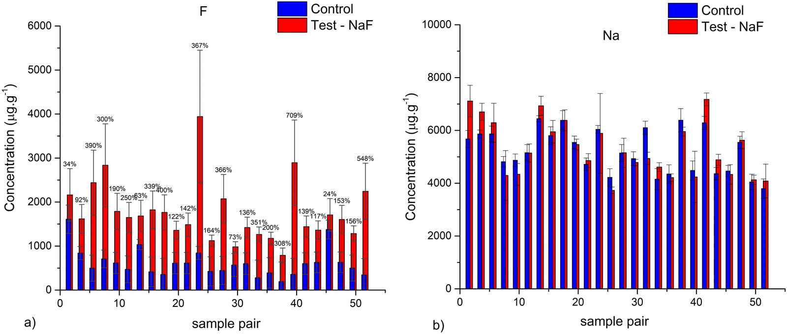

Fig. 1 Comparison of the (a) fluorine and (b) sodium concentration obtained for all the studied samples. Error bars correspond to the maximum deviation to the average value for the three measurements.

In order to further evaluate the chemical alterations in the structure of the samples we performed NEXAFS. Fig. 2a presents the comparison of NEXAFS spectra at the F K-edge of the control and test samples. Both spectra are characterized by an intense peak around ca. 688 eV and a variety of mostly smaller peaks at higher energies. In the F K-edge NEXAFS spectrum of the control sample main spectral features at ca. 687.5 and 690.9 eV can be observed, as well as a shoulder at ca. 695–696 eV. The shape of the spectra as well as its characteristic features fit very well with the literature references of the fluorapatite one.⁴² It is worth noting that the well-defined structure at 707–712 eV is related to Fe L_2,3-edge transitions arising from natural iron incorporation in the enamel matrix.⁴³ The F K-edge NEXAFS spectrum of the treated sample exhibits peaks at ca. 688, 691.3, 694.7, 697.8, 702.8, and 706.2 eV and broader structures at higher energies. It corresponds very nicely to the literature data on the CaF₂.⁴⁴

Fig. 2 Comparison of the NEXAFS spectra at the F K-edge obtained for (a) the control and test groups, and (b) the control group and simulated spectrum of Ca₅(PO₄)₃F and (c) the test group and simulated spectrum for CaF₂.

Fig. 2b and c compare the obtained spectra with the simulated spectra with more similar features. In this way, the obtained results showed that control samples were similar to fluorapatite, as a result of a low concentration fluoride uptake in enamel, from either systemic or topical sources.⁸ On the other hand, test samples present a NEXAFS spectrum with similar features as calcium fluoride. Factors relevant to the deposition of this product in vitro can be increased time of exposure, increased concentration, lowered pH, saliva and calcium pre-treatment.⁸ The paste was applied according to the manufacturer's indications, in air, without saliva, however the increased fluoride concentration of the NaF paste, was favorable to the formation of CaF₂.

Fig. 3a demonstrates the Ca-L_2,3 edge of treated and control samples. Both spectra consist of two main L₃ and L₂ (spin–orbit related peaks), together with two smaller peaks (A1, A2, and B1, B2) preceding the L₃ and L₂ edges, respectively, with the difference between A1-L₃, and B1–L₂ being higher than between A2-L₃ and B2-L₂.

Fig. 3 Comparison of the NEXAFS spectra at the Ca L-edge obtained for (a) the control and test groups, (b) the control group, Hap and Fap simulated spectra and (c) the test group, CaF₂ reference sample and simulated spectrum.

This multi-peak pattern originates from the crystal field splitting and is related to the symmetry of the atoms neighboring the Ca²⁺ ion in the first co-ordination sphere. It is well established that spectral intensity, number of visible peaks as well as the energy separation between the pre-peaks and the major features are unique and can serve as a fingerprint for the certain Ca-containing compounds.⁴⁴ The spectra of the treated and control samples are obviously characterized by different values of the peaks splitting in L₃ and L₂ edges. For the control sample the b2–b1 separation is 1.1 eV that fits well with the simulated data for FAp (Fig. 3b) and appears shifted by 0.3 eV for HAp.⁴⁴ Regarding the treated samples, spectra show features at the same energy positions as the CaF₂ reference sample, while A2 and B2 are more separated in energy from the respective L₃ and L₂ edges in the simulated CaF₂ spectra (Fig. 3c).

Regarding the Raman spectra, Fig. 4 shows a comparison of the Raman spectra for the control and test paired samples, and we could identify differences in less intense peaks attributed to symmetric bending vibrations and asymmetric stretching vibrations, namely, shifts in the peak's centroid or intensity. However, considering the NEXAFS results, and in a first attempt to analyze and compare the samples, the characteristic band of CaF₂ at ∼322 cm⁻¹ could not be identified in the test group. Taking into account the probed volume of the Raman measurements (considering the wavelength of the laser and N.A. of the lens) the depth of measurements should be to 1.1 μm.⁴⁵ This is much higher than the NEXAFS probed volume (up to 100 nm⁴⁶ in fluorescence mode) indicating that the formation of CaF₂ should occur superficially.

Fig. 4 Comparison of the Raman spectra for the control and test samples. As an inset, it is highlighted the slight shift for the symmetric stretching band of phosphate.

It was thought that calcium fluoride formation on enamel was unfavorable because it dissolves readily in saliva. However, research shows that at neutral pH, calcium fluoride is quite insoluble and can remain on tooth surfaces for weeks after fluoride application. This stability is attributed to the adsorption of secondary phosphate (HPO₄²⁻) and pellicle proteins on its surface. During acidic conditions, such as a caries attack, primary phosphate (H₂PO₄⁻) dominates, leading to calcium fluoride dissolution. The fluoride released under these conditions is incorporated into hydroxyapatite, reinforcing enamel. Afterwards, calcium fluoride is restabilized by secondary phosphate and proteins, serving as a pH-controlled fluoride reservoir.⁸

Table 1 presents the statistical analysis of the different parameters extracted from the spectra. As can be seen, for all parameters, the differences found between the control group and the test group are not significant.

Table 1 Descriptive statistics of the different parameters extracted from the Raman spectra

Band	Feature	Sample	Mean	SD	Minimum	Median	Maximum	p value
PO4^3− V1	Position	Control	964.7	0.3	964.1	964.8	965.4	0.44
		Test – NaF	964.8	0.2	964.4	964.8	965.2
	FWHM	Control	16.3	0.2	16.0	16.2	17.1	0.28
		Test – NaF	16.4	0.4	15.9	16.2	17.5
	Intensity	Control	17.8	0.2	17.4	17.8	18.5	0.15
		Test – NaF	17.7	0.3	16.9	17.7	18.5
	Depolarization ratio	Control	0.6	0.1	0.5	0.6	1.0	0.90
		Test – NaF	0.6	0.2	0.3	0.6	1.0
PO4^3− V2	Position	Control	445	2	441	444	447	0.27
		Test – NaF	444	2	440	444	449
	FWHM	Control	30	3	27	29	39	0.22
		Test – NaF	30	2	27	30	35
	Intensity	Control	6.1	0.5	5.3	6.0	7.3	0.34
		Test – NaF	6.4	0.6	5.6	6.4	8.4
CO3^2− V1	Position	Control	1068	4	1029	1049	1056	0.71
		Test – NaF	1070	20	1034	1048	1142
	FWHM	Control	47	6	34	48	56	0.65
		Test – NaF	48	9	32	46	77
	Intensity	Control	2.0	0.2	1.7	2.0	2.5	0.36
		Test – NaF	2.1	0.2	1.8	2.1	2.7
PO4^3− V4	Position	Control	586	1	584	586	589	0.3
		Test – NaF	587	2	584	587	593
	FWHM	Control	20	5	15	18	37	0.19
		Test – NaF	21	8	17	19	58
	Intensity	Control	4.5	0.7	3.7	4.3	6.6	0.09
		Test – NaF	5	2	3	5	13

---

To further evaluate the differences and try to discriminate between groups, principal components analysis was performed. Fig. 5a and b present the PCA score plots obtained using the full preprocessed spectra and the features extracted from the spectra. As can be seen, both approaches presented a high overlap of the scores for the control and test groups with variance explained by PC 1 of little over 40%. On the other hand, a cumulative explained variance of 93% is obtained by the 3^rd PC for approach A – the full spectrum, while this percentage of explained variance is only obtained by the 4^th PC when considering the spectral features extracted. This might be indicative that other features of the spectrum, besides the main phosphate and carbonate vibrational bands are informative to better characterize the samples.

Fig. 5 PCA plots obtained using (a) the whole spectrum and (b) selected features.

Although PCA is capable of identifying some important structural information in the data it has less discrimination power due to the fact that it is an unsupervised procedure. It does not identify features or patterns that are important for discriminating between groups, rather it extracts new features that compactly represent the data.³⁰ Often, the interpretation of the complex biochemical information obtained through vibrational spectroscopic techniques requires further data analysis using supervised procedures, such as, the RF classifier. Table 2 presents the performance metrics for the used RF classifiers following approaches A and B. For both approaches, the classifier achieved a good predictive performance, being able to distinguish whether samples underwent treatment or not.

Table 2 Performance metrics for the used RF classifiers following approaches A (full spectrum) and B (derived parameters)

	Group	Approach A	Approach B
Precision	Control	100	80
	Test – NaF	80	100
Recall	Control	75	100
	Test – NaF	100	75
F1-score	Control	86	89
	Test – NaF	89	86
Accuracy		87.5	87.5

---

Conclusion

This study demonstrates a comprehensive approach to evaluating fluoride uptake in human enamel, integrating advanced analytical techniques with machine learning for improved insight. Through the combined use of particle-induced gamma-ray emission (PIGE), near edge X-ray absorption fine structure (NEXAFS), and Raman spectroscopy, we quantitatively and qualitatively assessed fluoride uptake and the formation of fluoride-based compounds. PIGE analysis revealed a significant increase in fluoride concentration, ranging from a 39% increase to 709% increase in treated samples, confirming the effectiveness of NaF in enhancing fluoride retention within the enamel matrix. NEXAFS further substantiated the formation of CaF₂, highlighting its role as a stable fluoride reservoir in treated samples.

A key advancement in this study lies in the application of machine learning algorithms, particularly random forest classifiers, to Raman spectral data for distinguishing between treated and untreated enamel samples. By extracting spectral features, such as band intensity, full-width at half maximum (FWHM) of specific Raman peaks, and depolarization ratios, we demonstrated that machine learning algorithms can effectively differentiate subtle chemical and structural changes induced by fluoride treatment. This data-driven approach not only revealed previously unappreciated patterns within the spectra but also showed that even slight variations in vibrational modes could serve as reliable indicators of fluoride uptake. The supervised machine learning models achieved robust classification performance, confirming their utility in the context of spectral analysis for biomaterials research.

The integration of these methods underscores the potential of machine learning in enhancing the interpretation of Raman spectra, especially in complex biological samples where overlapping signals and subtle spectral shifts present challenges to traditional analysis. By streamlining the process of feature extraction and analysis, machine learning can provide a powerful tool for rapid screening and evaluation of dental treatments.

In conclusion, this multi-technique approach establishes a reproducible framework for assessing fluoride uptake in enamel and highlights the transformative role of machine learning in advancing Raman spectroscopic analysis. Future research may explore the application of this methodology to in vivo studies, aiming to refine predictive models and investigate the long-term stability of fluoride uptake in dental enamel. These findings have important implications for preventive dentistry, as they support the development of targeted fluoride treatments that optimize enamel remineralization and caries resistance.

Data availability

Data will be available upon reasonable request.

Conflicts of interest

There are no conflicts to declare.

Acknowledgements

This work has been financially supported by Fundação para a Ciência e a Tecnologia through the LIBPhys funding UID/FIS/04559/2020 and S. Pessanha contract CEECIND/00278/2018/CP1564/CT0007, https://doi.org/10.54499/CEECIND/00278/2018/CP1564/CT0007. Also, Marta B. Lopes acknowledges FCT for CEECINST/00042/2021, UIDB/00297/2020 and UIDP/00297/2020 (NOVA Math, Center for Mathematics and Applications). UIDB/00667/2020 and UIDP/00667/2020 (UNIDEMI). We thank the Helmholtz-Zentrum Berlin für Materialien und Energie for the allocation of synchrotron radiation beamtime at GELEM Dipole. GELEM-PES Endstation at HZB received funding from the BMBF program ErUM-Pro.

References

1. R. J. Lamont and P. G. Egland, Mol. Med. Microbiol., 2015, 2, 945–955,  DOI:10.1016/B978-0-12-397169-2.00052-4.
2. L. Guo, W. Hu, X. He, R. Lux, J. McLean and W. Shi, PloS One, 2013, 8, e57182,  DOI:10.1371/journal.pone.0057182.
3. J. D. B. Featherstone and A. Lussi, Understanding the chemistry of dental erosion, Monogr. Oral Sci., 2006, 20, 66–76,  DOI:10.1159/000093351.
4. Y. G. de Sousa Né, D. Souza-Monteiro, D. R. Frazão, M. O. P. Alvarenga, W. A. B. Aragão, N. C. F. Fagundes, R. D. de Souza-Rodrigues and R. R. Lima, PeerJ Inc., 2022, 10, e13864,  DOI:10.7717/peerj.13864.
5. R. F. Zanatta, D. M. D. S. Ávila, K. M. Miyamoto, C. R. G. Torres and A. B. Borges, Caries Res., 2019, 53, 1–9,  DOI:10.1159/000488207.
6. A. I. Ismail, J. Dent. Educ., 2004, 83, 56–66,  DOI:10.1177/154405910408301s12.
7. E. Medjedovic, S. Medjedovic, D. Deljo and A. Sukalo, Materia Socio Medica, 2015, 27, 395,  DOI:10.5455/msm.2015.27.395-398.
8. K. Rošin-Grget, K. Peroš, I. Sutej and K. Bašić, Acta Med. Acad., 2013, 2013(42), 179–188,  DOI:10.5644/ama2006-124.85.
9. M. Campillo, P. D. Lacharmoise, J. S. Reparaz, A. R. Goñi and M. Valiente, J. Chem. Phys., 2010, 132, 244501,  DOI:10.1063/1.3428556.
10. K. Herman, M. Wujczyk, M. Dobrzynski, D. Diakowska, K. Wiglusz and R. J. Wiglusz, Materials, 2021, 14, 3747,  DOI:10.3390/ma14133747.
11. L. Bubnowicz and R. França, Appl. Surf. Sci. Adv., 2022, 11, 100306,  DOI:10.1016/j.apsadv.2022.100306.
12. N. Pai, J. Mcintyre, N. Tadic and C. Laparidis, Aust. Dent. J., 2007, 52, 41–46,  DOI:10.1111/j.1834-7819.2007.tb00464.x.
13. P. Seredin, D. Goloshchapov, Y. Ippolitov and J. Vongsvivut, Sci. Rep., 2020, 10, 20891,  DOI:10.1038/s41598-020-78078-8.
14. S. Pessanha, S. Silva, J. M. Silveira, I. Otel, H. Luis, V. Manteigas, A. P. Jesus, A. Mata and M. Fonseca, Spectrochim. Acta, Part A, 2020, 236, 118378,  DOI:10.1016/j.saa.2020.118378.
15. V. Cavalli, D. A. da Rosa, D. P. da Silva, M. Kury, P. C. S. Liporoni, L. E. S. Soares and A. A. Martins, J. Appl. Oral. Sci., 2018, 26, e20170589,  DOI:10.1590/1678-7757-2017-0589.
16. I. Otel, K. Dias, R. Pereira, M. Fonseca, A. P. Jesus, A. Mata, V. Vassilenko, J. M. Silveira and S. Pessanha, J. Trace Elem. Med. Biol., 2022, 71, 126938,  DOI:10.1016/j.jtemb.2022.126938.
17. A. S. Hardikar, N. N. Gaonkar, S. N. Devendrappa, T. S. Machindra and S. Hadkar, Int. J. Clin. Pediatr. Dent., 2023, 16, 363–370,  DOI:10.5005/jp-journals-10005-2535.
18. G. Luís, H. Silva, J. Silveira, V. Manteigas, A. Mata, D. Marques, A. Jesus, M. Fonseca and S. Pessanha, J. Raman Spectrosc., 2018, 50, 380–386,  DOI:10.1002/jrs.5532.
19. T. Bocklitz, A. Walter, K. Hartmann, P. Rösch and J. Popp, Anal. Chim. Acta, 2011, 704, 47–56,  DOI:10.1016/j.aca.2011.06.043.
20. Y. Qi, D. Hu, Y. Jiang, Z. Wu, M. Zheng, E. X. Chen, Y. Liang, M. A. Sadi, K. Zhang and Y. P. Chen, Adv. Opt. Mater., 2023, 11, 2203104,  DOI:10.1002/adom.202203104.
21. S. Pessanha, I. Otel, V. Vassilenko, J. M. Silveira and P. Ribeiro, J. Raman Spectrosc., 2024, 55, 975–981,  DOI:10.1002/jrs.6704.
22. M. K. M. Ferreira, D. Souza-Monteiro, L. O. Bittencourt, J. M. Matos-Sousa, V. S. Chemelo, V. R. N. Santos, P. B. O. Nunes, G. de, S. Balbinot, A. F. Prado, F. M. Collares, F. J. Ager, I. Ortega-Feliu, M. A. Respaldiza, S. Pessanha and R. R. Lima, Chemosphere, 2022, 307, 136053,  DOI:10.1016/j.chemosphere.2022.136053.
23. Y. Funato, Y. Matsuda, K. Okuyama, H. Yamamoto, H. Komatsu and H. Sano, Dent. Mater. J., 2015, 34, 240–245,  DOI:10.4012/dmj.2014-127.
24. O. V. Petrova, S. V. Nekipelov, D. V. Sivkov, A. E. Mingaleva, A. Nikolaev, O. V. Frank-Kamenetskaya, V. V. Bazhenov, D. V. Vyalikh, S. L. Molodtsov, V. N. Sivkov and H. Ehrlich, J. Phys. Conf. Ser., 2017, 917, 042001,  DOI:10.1088/1742-6596/917/4/042001.
25. D. Goloshchapov, N. Buylov, A. Emelyanova, I. Ippolitov, Y. Ippolitov, V. Kashkarov, Y. Khudyakov, K. Nikitkov and P. Seredin, Nanomaterials, 2021, 11, 3099,  DOI:10.3390/nano11113099.
26. J. M. Silveira, S. Coutinho, D. Marques, J. Castro, A. Mata, M. L. Carvalho and S. Pessanha, Spectrochim. Acta, Part A, 2018, 198, 145–149,  DOI:10.1016/j.saa.2018.03.007.
27. G. Pezzotti, T. Adachi, I. Gasparutti, G. Vincini, W. Zhu, M. Boffelli, A. Rondinella, E. Marin, H. Ichioka, T. Yamamoto, Y. Marunaka and N. Kanamura, Spectrochim. Acta, Part A, 2017, 173, 19–33,  DOI:10.1016/j.saa.2016.08.036.
28. J. P. Hirvonen, Handbook of Modern Ion Beam Material Analysis, Material Research Society, Pittsburg, 1995.
29. J. F. Ziegler, Nucl. Instrum. Methods Phys. Res., Sect. B, 2004, 219–220, 1027–1036,  DOI:10.1016/j.nimb.2004.01.208.
30. R. Gautam, S. Vanga, F. Ariese and S. Umapathy, EPJ Tech. Instrum., 2015, 2, 8,  DOI:10.1140/epjti/s40485-015-0018-6.
31. H. Kinoshita, N. Miyoshi, Y. Fukunaga, T. Ogawa, T. Ogasawara and K. Sano, J. Raman Spectrosc., 2008, 39, 655–660,  DOI:10.1002/jrs.1908.
32. J. Mihály, V. Gombás, A. Afishah and J. Mink, J. Raman Spectrosc., 2009, 40, 898–902,  DOI:10.1002/jrs.2194.
33. T. Buchwald, Z. Okulus and M. Szybowicz, J. Raman Spectrosc., 2017, 48, 1094–1102,  DOI:10.1002/jrs.5175.
34. S. I. Fedoseenko, D. V. Vyalikh, I. E. Iossifov, R. Follath, S. A. Gorovikov, R. Püttner, J. S. Schmidt, S. L. Molodtsov, V. K. Adamchuk, W. Gudat and G. Kaindl, Nucl. Instrum. Methods Phys. Res., Sect. A, 2003, 505, 718–728,  DOI:10.1016/S0168-9002(03)00624-7.
35. O. Bunǎu and Y. Joly, J. Phys.: Condens. Matter, 2009, 21, 345501,  DOI:10.1088/0953-8984/21/34/345501.
36. S. A. Guda, A. A. Guda, M. A. Soldatov, K. A. Lomachenko, A. L. Bugaev, C. Lamberti, W. Gawelda, C. Bressler, G. Smolentsev, A. V. Soldatov and Y. Joly, J. Chem. Theory Comput., 2015, 11, 4512–4521,  DOI:10.1021/acs.jctc.5b00327.
37. I. T. Jolliffe, Principal Component Analysis, Springer, 2^nd edn, 2002.
38. E. Timchenko, P. Timchenko, L. Volova, O. Frolov, M. Zibin and I. Bazhutova, Diagnostics, 2016, 769, 012047,  DOI:10.3390/diagnostics10110876.
39. L. Breiman, Random Forests, 2001, vol. 45, pp. 5–32 DOI:10.1023/A:1010933404324.
40. W. Zhang, C. M. Giang, Q. Cai, B. Badie, J. Sheng and C. Li, Mach. Learn.: Sci. Technol., 2023, 4, 045053,  DOI:10.1088/2632-2153/ad1349.
41. A. Amjad, R. Ullah, S. Khan, M. Bilal and A. Khan, Vib. Spectrosc., 2018, 99, 124–129,  DOI:10.1016/j.vibspec.2018.09.003.
42. C. A. Stifler, N. K. Wittig, M. Sassi, C. Y. Sun, M. A. Marcus, H. Birkedal, E. Beniash, K. M. Rosso and P. U. P. A. Gilbert, J. Am. Chem. Soc., 2018, 140, 11698–11704,  DOI:10.1021/jacs.8b05547.
43. S. Pessanha, S. Coutinho, M. L. Carvalho, J. M. Silveira and A. Mata, Spectrochim. Acta, Part B, 2017, 138, 8–13,  DOI:10.1016/j.sab.2017.10.001.
44. P. Roesch, C. Vogel, T. Huthwelker, P. Wittwer and F. G. Simon, Environ. Sci. Pollut. Res., 2022, 29, 26889–26899,  DOI:10.1007/s11356-021-17838-z.
45. P. Dhamelincourt, Raman Microscopy in Handbook of Vibrational Spectroscopy, 2002 DOI:10.1002/0470027320.
46. B. L. Henke, E. M. Gullikson and J. C. Davis, At. Data Nucl. Data Tables, 1993, 54, 181–342,  DOI:10.1006/adnd.1993.1013.

---

Footnote

† Electronic supplementary information (ESI) available. See DOI: https://doi.org/10.1039/d5tb00213c

---