Spatial correlation of desorption events accelerates water exchange dynamics at Pt/water interfaces

Abstract

The altered solvation structures and dynamical properties of water molecules at the metal/water interfaces will affect the elementary step of an electrochemical process. Simulating the interfacial structure and dynamics with a realistic representation will provide us with a solid foundation to make a connection with experimental studies. To surmount the accuracy-efficiency tradeoff and provide dynamical insights, we use state-of-the-art machine learning molecular dynamics (MLMD) to study the water exchange dynamics, which are fundamental to adsorption/desorption and electrochemical reaction steps. We reproduce interfacial structures consistent with ab initio molecular dynamics (AIMD) results and obtain diffusion and reorientation dynamics in agreement with the experiment. We show that the hydrogen bonds at the interface become stronger than those in bulk water, which makes the diffusion, reorientation, and hydrogen-bond dynamics slower. Our findings reveal that the spatial correlation of desorption events, driven by the breaking and making of hydrogen bonds, accelerates water exchange dynamics. These dynamics occur on timescales of several hundred picoseconds at 337 K and 302 K. We take a solid step forward toward studying the in situ interface water dynamics and attribute the fast water exchange dynamics to the spatial correlation of the desorption events.

---

1 Introduction

The significance of electrochemical reactions at solid/liquid interfaces is widely acknowledged due to their important roles in various industrial applications, such as electrocatalysis, electrolysis, and corrosion.¹ To study the electrochemical reactions, the Gouy–Chapman–Stern (GCS) model has been established as a well-known phenomenological model.^2–6 A molecular-level understanding of interfacial phenomena necessitates the integration of microscopic information into the GCS model. Therefore, many in situ spectroscopic techniques have been developed to characterize the microscopic structures at the metal/water interfaces, for example, surface X-ray scattering spectroscopy to measure the water density profile,⁷ X-ray absorption spectroscopy to investigate the hydrogen bond structure,⁸ and in situ Raman spectroscopy to study the structural change.⁹ Aside from probing the interfacial structures, developing microscopic techniques with high temporal and spatial resolution to study the interfacial dynamics represents a frontier research topic.^10,11 For example, Lapointe et al. demonstrated that the ultrafast dynamics of a hydrated electron at the metal/electrolyte interface can be followed with a resolution in the tens of femtoseconds using a pump–push–probe scheme.¹² The hierarchical interfacial dynamics expanding from a few femtoseconds to several microseconds can fundamentally affect the electrochemical reaction mechanisms. However, the state-of-the-art techniques to characterize the interfacial dynamics can only provide limited information at the metal/water interfaces.¹³ This limitation underscores the importance of molecular dynamics simulations in advancing our understanding of interfacial dynamics.

Of the many simulations of the interfacial dynamics (i.e. electron transfer,¹⁴ proton-coupled electron transfer^15,16), water exchange dynamics are of fundamental interest as this process constitutes the thermodynamic and kinetic basis of many elementary steps. Limmer and Willard et al.^17–19 studied the water exchange dynamics at the Pt/water interfaces using classical molecular dynamics and suggested the timescale to be over several nanoseconds at 298 K. Nevertheless, the high water coverage (approximately 0.85 monolayer) and oxygen density profiles at the Pt/water interfaces are distinct from the results of ab initio molecular dynamics (AIMD)²⁰ simulations. For AIMD simulations, observations of water exchange at the interfaces are reported^21,22 within 40 picoseconds. Nevertheless, the samplings are deemed insufficient for capturing the full picture of the dynamics of water exchange. Aside from the efficiency issue, the choice of functionals^23–25 and thermostats^26–28 is also reported to affect the structural dynamics, making the comparison of different theoretical efforts and the connection to experimental studies less clear.

To address the sampling issues we conducted machine learning molecular dynamics (MLMD) simulations and compared the oxygen density distributions from MLMD with those from previous AIMD simulations.²⁹ We also made a benchmark comparison of the pure bulk water dynamics between MLMD and experimental observations, which reveals that by increasing the MD temperature by approximately 50 ± 10 K, the PBE-D3 predictions regarding the water dynamics closely align with the experimental results of the diffusion dynamics³⁰ and reorientation dynamics.^31,32 Based on the above theoretical calibration of the simulation temperature, we determine the residence timescale to be a few hundred picoseconds for water at the Pt/water interfaces at 337 and 302 K, which is much faster than classical MD results.¹⁹ This heightened frequency of water exchange underscores the critical importance of explicitly considering interface dynamics, especially in scenarios where water functions as a reacting species. For example, the probability of the first peak of adsorbed water dissociation may be suppressed if the water molecules are exchanged to the bulk region, which is closely related to the interfacial neutral pH. We reveal that the acceleration of water exchange is driven by the correlation between initial and subsequent desorption events, and this correlation is key to the observed acceleration. This correlation primarily operates within the first solvation shell of water molecules and during the first few picoseconds following the initial desorption event. This research significantly advances our comprehension of the dynamics of water exchange at metal/water interfaces.

2 Computational details

2.1 Models and computations

An orthogonal 4 × 4 × 6 model for the Pt(100)/water interface and a non-orthogonal 6 × 6 × 6 model for the Pt(111)/water interface were constructed, with 6 atomic Pt slabs and water molecules filled in between the top and bottom of the Pt surfaces. The lattice parameter for the supercell is 11.246, 11.246 and 35.94 Å (16.869, 16.869 and 41.478 Å) in the x/y/z direction. Here, the water density has been determined to be 0.97 g cm⁻³ at the middle 10 Å for the Pt(100)/water interface. The water density for the Pt(111)/water interface is around 1.00 g cm⁻³ at the middle 10 Å. For the production run, we expand both the models to orthogonal 8 × 8 × 6 Pt slabs as shown in Fig. 1. For pure bulk water, a cubic box containing 128 water molecules was constructed with L equal to 15.65 Å.

Fig. 1 Schematic illustration of the construction, validation, and application of the machine learning potential (MLP). The definitions of A, B, C, and L are as follows: A (below 2.65 Å), B (2.65–4.5 Å), C (4.5–6.8 Å), and L denote the water molecules within the middle 5 Å of the interface models. All the distances are referenced to the Pt surfaces in contact with water molecules. Here, two machine learning potentials are trained for each system, separately.

All the density functional theory (DFT) calculations are performed in CP2K/Quickstep.³³ The Goedecker–Teter–Hutter (GTH) pseudopotentials^34,35 are used to describe the atoms: H is described by GTH-PBE-q1, with all electrons in the valence, the O atom is described by GTH-PBE-q6 with 2s and 2p electrons in the valence, and Pt is described by Pt GTH-PBE-q10 with 5d and 6s electrons in the valence. The DZVP-MOLOPT-SR-GTH Gaussian basis³⁶ set is used for all atom types except for Pt, which uses a developed basis set for the GTH-PBE-q10 of Pt by Le et al.²⁰ The cutoff of the plane wave energy is set to 1000 Ry. The Perdew–Burke–Ernzerhof (PBE) functional is utilized to describe the exchange-correlation effect.³⁷ Grimme D3 correction is included to consider the dispersion interaction.³⁸

2.2 Machine learning potential and MD simulations

We utilize the DPGEN workflow to iteratively update the training dataset for developing machine learning potentials. This workflow consists of three main parts: training, exploration, and labeling. Detailed descriptions can be found in the original literature.^39,40 Utilizing this workflow, we have updated the dataset of interfacial structures to 4300 for Pt(111)/water and 4370 for Pt(100)/water. To conduct MD simulation with ab initio accuracy and high efficiency, we use the deep potential model to learn the structure-dependent energies and forces. The se_a descriptor is used in this work.⁴⁰ The training process contains two sets of deep neural networks: the embedding network for training descriptors and the fitting network for training MLPs. The size of embedding networks is set to (25, 50, 100) and that of the fitting network is set to (240, 240, 240). The cutoff radius of descriptors is set to 8.0 Å and the weight decays smoothly from 0.5 to 8.0 Å. The test of r_cut can be found in the ESI (Fig. S4†). For the active learning process, 200 000 steps are used to train the potential. For the final production of MLPs, 2 000 000 steps are used.

The molecular dynamics (MD) simulations are performed with both the Large-scale Atomic/Molecular Massively Parallel Simulator (LAMMPS) package⁴¹ and CP2K package.³³ For the exploration in the DPGEN, we use LAMMPS to conduct MD. The simulation is conducted in the NVT ensemble and we set the temperature to 330/430/530 K to include the configurations distributed around these temperatures. The time step is set to 0.5 fs and the Nose–Hoover thermostat is used to control temperature with the temperature damping parameter setting to 100 fs.^42,43 For the equilibration and production run, we used the CP2K package. For the convenience of comparison to previous ab initio molecular dynamics (AIMD) simulations,^29,44 we performed second-generation Car–Parrinello MD in a canonical ensemble (NVT) using a time step of 0.5 fs. The Langevin friction coefficient γ_D is set to 0.001 fs⁻¹. The intrinsic friction coefficients γ_L are set to 2.2 × 10⁻⁴ fs⁻¹ for H₂O and 5 × 10⁻⁵ fs⁻¹ for Pt based on preliminary tests.⁴⁴ The validation runs involve performing a 1 ns simulation using the MLP with K point correction included. Then, we extracted 200 structures and calculated their energy and force using the first-principles calculations (2 × 2 × 1 k point setup). We compared the RMSE (root mean square error) of the energy and force to those determined by the MLP. The results are shown in ESI Table S1† (columns 5 and 7). To determine whether the thermostat affects the intrinsic dynamics, we conducted a subsequent 10 ns MD simulation in the NVE ensemble after 10 ns simulations in the NVT ensemble.

2.3 K point correction

Our test shows that the energy and force will gradually converge when we increase the k point density. But, the high k-point density will be very expensive to label the data. Here, we propose a K point correction scheme. In this scheme, we first test the energy convergence over different k-point grids. It is observed that 2 × 2 × 1 is good enough with the RMSE of energy smaller than 1 meV per atom. Then we get the energy/force difference determined by a 2 × 2 × 1 k point setup and gamma point. Finally, we learn this difference using the se_a descriptor. After testing and validating this newly trained potential over a series of structures, we get a stable MLP (machine learning potential) to predict the energy/force difference between gamma point and a converged k grid setup. Using this MLP, we can get the difference of all the structures that are initially labeled by gamma point. Then we add this difference to the gamma point labelled data. The tests are shown below. It can be seen that this correction lowers the RMSE of energy and force, which could give a better description of expanded models. With the above correction, we trained MLPs for Pt(100)/water and Pt(111)/water interfaces, respectively. The RMSE for energy and force can be found in ESI Table S1† for both systems.

2.4 Formulae for statistical analysis

The one-dimensional diffusion coefficient is obtained based on the mean square displacement (MSD):

The three-dimensional diffusion coefficient is obtained based on the mean square displacement (MSD):

We used the three-dimensional formula to determine the diffusion coefficients for pure bulk water molecules. The finite size correction to the diffusion coefficients was estimated using the expression proposed by Dünweg and Kremer:^45,46. Here k_B is the Boltzmann constant, T is the temperature, ζ equals 2.83729, and η is the viscosity of liquid water whose value was taken from experimental data. L is the size of the cubic simulation cell.

The hydrogen-bond dynamic correlation function is defined as follows:

where the operator h(t) is one if the hydrogen bond criterion is met. a(0) is 1 if the water molecules are in a specific region. The timescales used to do correlation function analyses at different temperatures can be found in ESI Table S3.† The dipole–dipole auto-correlation function is as shown below:

C_rot(t) = 〈P_l(μ(t)a(0)μ(0))〉 (4)

where μ(t) represents the dipole orientation at time t of all water molecules in a specific region. a(0) is 1 if the water molecules are in a specific region. P_l is the lth degree Legendre polynomial. The sum of the vector product is normalized over the initial vector. The residence time correlation function is defined as below:where h(0) is 1.0 if the water molecules are situated in the specified region and 0.0 otherwise. h(t) is 1.0 if it meets the standard at the time interval t and 0.0 if not. The result is averaged over all the molecules at the time origin. Following the definition of Limmer et al., the flux correlation function is defined as:where h(0) is 1.0 if the water molecules are situated in the initial region and g(t) is 1.0 if the original water molecules are in the final region. The result is also averaged over all the molecules at the time origin. Here we use the vertical distance centers between the peaks and valleys to define the stable region. Now, A is 1.8 to 2.45 Å. B is 2.9 to 3.8 Å. L is 5.2 to 12.75 Å.

The vertical distances of the peaks and valleys of the oxygen density profile are used to distinguish water molecules in different regions. To study the residence dynamics and avoid the inclusion of water molecules that are at the boundary of different adsorption peaks, we use the middle values between the peaks and valleys. For example, the first chemisorbed peak is at around 2.3 Å and the first valley is at around 2.65 Å. So, we use 2.45 Å as the plane to choose those water molecules in the chemisorbed state in the A region. Based on these distinct regions, we conduct the residence correlation function analysis.

3 Results and discussion

3.1 Validation of the machine learning potential

First, we extracted 200 initial structures (Fig. S1†) from AIMD simulations for Pt(111) and Pt(100)/water interfaces.²⁹ Then we started the active learning process using the DPGEN workflow.³⁹ This workflow contains three parts: training, exploration, and labeling. After updating the dataset to achieve low RMSE for energy and force (Fig. S2, S3 and Table S1†), we implemented a k-point density correction scheme (see Methods and Fig. S4†) to enhance the machine learning potential (MLP) performance. Using this corrected MLP and expanded interface models, we conducted MLMD. We compare the oxygen density distribution profiles from our MLMD and previous AIMD simulations.²⁹ The RMSE values are below 0.60 meV per atom for energy and 80 meV Å⁻¹ for forces (Fig. S1–S4 and Table S1†). Additionally, the temperature in the NVT ensemble and total energy in the NVE ensemble during the 10 ns simulations for both systems can be referenced in Fig. S5 and S6.† No systematic energy drift is observed in the NVE simulation, confirming the robustness of the MLPs. From the oxygen density distributions derived from the MLMD and AIMD,²⁹ we can see that the peak positions align consistently with previous AIMD simulations.²⁹ The first peak is identified at a vertical distance of 2.3 Å for both models, succeeded by a second peak at 3 Å for Pt(100) (3.1 Å for Pt(111)). A third peak is discernible at 5.9 Å, while valleys are observed at 2.65 Å and 4.5 Å. To investigate water exchange processes at the interface, we categorize water molecules into different regions: A (below 2.65 Å) representing the first peak adsorbed state, B for the second peak adsorbed state (2.65–4.5 Å), C (4.5–6.8 Å), and L denotes the water molecules within the middle 5 Å of the model. These classifications can also differentiate the OH vector and water bisector distributions along the surface normal (Fig. S7 and S8†), dividing them into distinct regions (Table S2†). Our subsequent analysis and exploration of dynamics will proceed according to the structural classification outlined above.

3.2 Benchmark comparison of water dynamics

As discussed in the introduction, direct detection of water dynamics at metal/water interfaces is limited by the constraints of detection resolution (both temporal and spatial). In contrast, the diffusion coefficients based on the high-temperature multinuclear-magnetic-resonance probe experiment³⁰ and reorientation lifetimes based on the THz spectroscopy⁴⁷ of liquid H₂O and D₂O are experimentally accessible. Therefore, we conduct a benchmark comparison of these properties by performing machine learning molecular dynamics simulations of pure bulk water with 128 water molecules in the simulation box. We use the mean squared displacement (MSD) method to calculate the diffusion coefficients and track the displacement every 10 ps over a 5 ns trajectory. We estimated the finite size correction to the diffusion coefficients as introduced above. For water reorientation dynamics, we analyzed the second Legendre polynomials of the correlation function associated with the water bisector as shown in eqn (4). We fitted the lifetime using two exponential forms. Fig. 2A shows the diffusion coefficients (red) and the fitted lifetime (orange) of water bisector reorientation dynamics over temperatures. The experimental data are extracted from previous publications^30,47 (black data points for reorientation dynamics and grey data points for diffusion dynamics). A 50 K temperature shift in our simulations aligns the trend of water diffusion coefficients over temperature with experimental data. This is similar to previous tests on MD simulations using the PBE functional, which suggested an increase of around 100 K (ref. 48) of the simulation temperature to match the experiment. For the reorientation dynamics, we observe that the slow lifetime fits well with the experiment after we shift the simulation temperature (see Fig. S13† for the comparison of a fast lifetime). The best fit is obtained by shifting the simulation temperature by 43 K. After the temperature shift, the reorientation lifetimes from the simulation at 302/337 K are about 2.5 ps faster than the experimental results.⁴⁷ Based on the above comparison, we assume that we can use PBE-D3 to study the water dynamics by increasing the simulation temperature by approximately 50 ± 10 K. A similar approach of shifting temperature to correct for functional errors has been often used in previous work.^48–51 In the following section, we present results from MLMD simulations where the temperature was adjusted by 50 K.

Fig. 2 (A) Benchmark comparison of water bisector reorientation dynamics and diffusion dynamics from simulations and experimental observations. (B) The oxygen diffusion along the surface from its original position within 20 ps for the Pt(100)/water interface. (C) Mean squared displacements (MSD) of the oxygen atom of water L parallel to the Pt surfaces. For the NVE ensemble, the subscript 1/2/3 stands for the three temperatures. (D) The diffusion coefficients for water B, C, and L of Pt(100) and Pt(111). The data of expt.^diff is reproduced with permission from ref. 30. The data of expt.^Rs is reproduced with permission from ref. 47.

3.3 Diffusion dynamics

Fig. 2B depicts the diffusion characteristics of water molecules along the surface over 20 ps, analyzing the movement of water's oxygen atom. Water molecules in region A exhibit localized movements near the apex of the Pt atom. In region B, water molecules are constrained by the hydrogen bond network formed by the relatively immobile water molecules in region A. As we move to region C, these constraints begin to diminish, with water in region L experiencing even less restriction in its movements.

For the interface models, we use the MSD method to calculate the diffusion coefficients and track the displacement every 10 ps over a 5 ns trajectory (Fig. 2C). Due to the isotropic diffusion along the surfaces on Pt(111)/Pt(100) surfaces that are different from the stepped Pt/water interface as we recently observed,⁵² we choose to show the one-dimensional diffusion. Here, we did not include the finite size correction as the correction is relatively small and the comparison between different types of water molecules makes the correction less important. The MSDs of water molecules L obtained from simulations in NVE ensembles for Pt(111) and Pt(100) are presented in Fig. 2C (see Fig. S17† for NVT results). We obtain the diffusion coefficients from the slope of the MSD over time. Here, we did not include the finite size correction as the target is to compare the relative trend of the diffusion dynamics. Fig. 2D shows the diffusion coefficients of water molecules in B, C, and L regions. Compared to the diffusion coefficients of pure bulk water molecules (Fig. 2A) at the respective temperature, the 1D diffusion coefficients of water L along the xy plane parallel to the Pt surface are faster by about 0.2/0.6/0.9 × 10⁻⁵ cm² s⁻¹ at 270/302/337 K, which is also observed in a previous study⁵³ and we attribute this difference to the confinement of the interfacial water molecules. Moving from region L to C and B (Fig. 2D), we observe a decrease in diffusion coefficients, with water B exhibiting nearly half the diffusion coefficient of water L. Taking the deviation into consideration, the diffusion coefficient difference between the Pt(111) and Pt(100) interfaces is mild. This trend aligns with observations on copper single crystal surfaces.⁵³ The distributions of diffusion coefficients are further detailed in Fig. S9.†

3.4 Hydrogen-bond and reorientation dynamics

The hydrogen-bond (HB) geometry formed between two water molecules is depicted in Fig. 3A, with d_OO set at 3.2 Å and θ at 30° for stable hydrogen bonds. We define a correlation function for hydrogen bonds (see the Computational details section) in specific regions, which tracks the duration of stable hydrogen bonds. This allows us to study the dynamics of hydrogen bonding within these regions. We then fit this correlation function using two exponential functions (Fig. S10†) to obtain the timescales associated with hydrogen bond changes as suggested by previous studies of bulk water molecules.^54,55 In this context, the mean and deviation values for the slow timescale are presented in the main text, while the results for the fast timescale can be referenced in Fig. S11.† In Fig. 3B, it is evident that the HB lifetime of pure bulk water increases from 2.4/6.6 ps at 337 and 302 K to 31.2 picoseconds at 270 K. A prior AIMD simulation of pure bulk water at 298 K, utilizing revised PBE with dispersion correction, determined a slow lifetime of approximately 18 ps (with d_OO set at 3.4 Å).⁵⁵ Moreover, an AIMD simulation at the coupled cluster level with an aug-cc-pVDZ basis set of pure water molecules suggested a slow hydrogen bond lifetime of 5.11 ps at 300 K.⁵⁴ The choice of parameters to define hydrogen bonds and time intervals to do correlation function analysis as well as the function forms to fit the lifetimes may affect the results in a minor way. The discrepancies between the revised PBE with dispersion correction and PBE-D3 suggest that these two functionals generally predict stronger hydrogen bonds than observed experimentally, leading to overestimation of their lifetimes. Neither functional matches the experimental results as well as high-level electronic theories. The fitted lifetime difference between bulk water and water L is minimal at both 337 K and 302 K. To better converge the analysis of the dynamics, we run 20 ns simulations at 270 K for each model in the NVE ensemble. The mean slow lifetime of water L in the Pt(100)/water model is approximately 10 ps shorter than that of bulk water. In the Pt(111)/water model, it is about 10 ps longer than that of bulk water. We attribute the difference in lifetime values observed across different models and ensembles to the water exchange dynamics at the interfaces. As shown in Table S3,† we track the hydrogen bond in the water L region by about 200 ps at 270 K, during which water molecules can leave the L region. This incorporates the hydrogen bond dynamics of interfacial water molecules into the fitted lifetime of water L. Interfacial water molecules in region AB (Fig. 3C) exhibit a longer HB lifetime, while those in region C (Fig. 3D) possess a lifetime comparable to those in region L at the respective temperatures. This suggests an exchange of water molecules between regions L and C. The observation that interfacial water molecules possess a longer HB lifetime aligns with the trend that interfacial water molecules exhibit lower diffusion coefficients.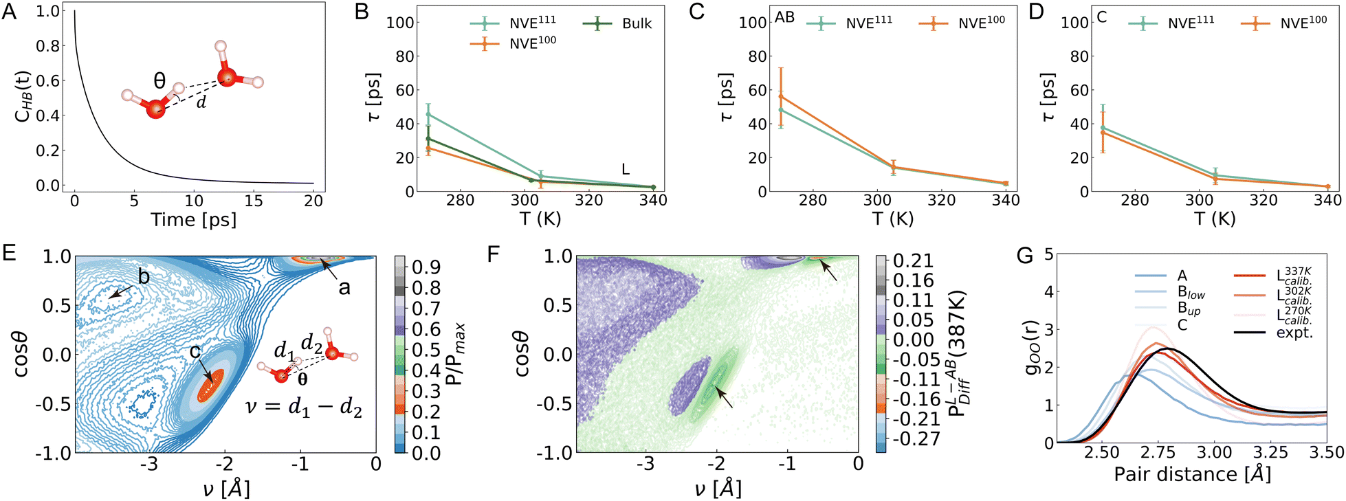

Fig. 3 (A) Hydrogen bond correlation function. C_HB(t) represents the hydrogen bond correlation function for water molecules in specific regions. The inset figure defines hydrogen bonds using the distance between two oxygen atoms and the angle between HO and OO′. The distance is set to 3.2 Å and the angle to 30°. (B–D) The fitted lifetime of the slow hydrogen bond dynamics of water L, AB, and C. See NVT results in Fig. S18.† (E) The joint probability distribution of finding an O–H–O′ geometry with a given ν–θ configuration for water molecules. Here, ν is the difference between the distance of OH and HO′. θ is defined as the angle between OH and OO′. Arrows are used to point to the stable/metastable geometry for a, b, and c. For the scale bar, P denotes the frequency count, and P_max represents the maximum frequency count of a given O–H–O′ geometry. P/P_max denotes the normalized probability distribution. (F) The difference between the normalized joint probability of water AB and L at 387 K. Arrows are used to indicate the main geometry difference at the interface. (G) The radial distribution function (RDF) for O–O of interfacial water molecules at 337 K and water L at 270/302/337 K. The experimental data is reproduced with permission from ref. 58.

To further investigate the trend of longer lifetimes observed for interfacial water molecules, we analyzed the joint probability distribution of the O–H–O′ geometry. As defined in the caption of Fig. 3, a more positive value of ν in the O–H–O′ geometry suggests a stronger hydrogen bond. Fig. 3E illustrates three geometry domains (a), (b), and (c), indicated by arrows. In domain (a), cos θ is nearly 1.0 and ν is close to −1.0 Å (Fig. S12A†), suggesting a strong hydrogen bond. In domain (b), cos θ is close to 0.60 and ν is close to −3.60 Å. This geometry does not correspond to a stable hydrogen bond between the observed donor and acceptor water molecules (Fig. S12B†). However, these donor water molecules may form hydrogen bonds with other surrounding water molecules. For geometry domain (c), the values of cos θ and ν are approximately −0.40 and −2.20 Å, respectively.⁵⁶ This hydrogen bond geometry involves donor water molecules (O) that accept hydrogen from defined acceptor water molecules (O′), but do not donate hydrogen to them (Fig. S12C†). An analysis of the disparity in joint probability between water molecules in the bulk and interface regions (Fig. 3F) reveals that hydrogen bonds in the interface (green) exhibit a more positive ν compared to those in the bulk region (purple). This observation is supported by the radial distribution function (RDF) of O–O, where the hydrogen bonds in the AB region are approximately 0.1 Å shorter than those in the L region (Fig. 3G). These findings highlight the distinct characteristics of interfacial water molecules: stronger hydrogen bonds with longer lifetimes, and lower diffusion coefficients. It should be further noted that PBE-D3 calculations predict a shorter O–O RDF peak compared to experimental observations.⁵⁷ By raising the simulated temperature by 50 K, a closer alignment of the peak position and height in the simulation results with the experimental data is achieved.⁵⁸

The reorientation of water molecules is intricately linked to the dynamic rearrangement and restructuring of the hydrogen bond (HB) network.⁵⁹ Studies have demonstrated that rotational anisotropy is directly related to the second-order rotational autocorrelation function of the transition dipole moment of excited molecules.³¹ To assess the reorientation dynamics at the interface, we analyzed the second Legendre polynomials of the correlation function associated with the water bisector, which closely aligns with the direction of the dipole moment.³² The same trajectory employed for the analysis of hydrogen bond dynamics was utilized to study the reorientation dynamics. Subsequently, a two-exponential form was employed to fit the correlation functions for water A, B, C, and L for Pt(100)/water and Pt(111)/water interfaces. Fig. 4A illustrates the slow lifetime of pure bulk water (blue) and water L for the reorientation dynamics as determined by MLMD (see Fig. S13† for a fast lifetime). Compared to pure bulk water (Fig. 4A, green, also shown in Fig. 2A, orange), the reorientation dynamics of water L exhibit a slower rate at 270 K. The lifetime of water L is approximately 10–15 ps, about 5 ps slower than that of bulk water at the Pt(111)/water and Pt(100)/water interfaces. The deviation between NVE and NVT results is approximately 5 ps (see Fig. S19† for NVT results). As with hydrogen bond dynamics, this difference is likely attributable to water exchange dynamics and the time interval used for reorientation correlation function analysis. At the other two temperatures, the lifetime difference between water L and pure bulk water is minor, a trend also observed for hydrogen bond dynamics and diffusion dynamics. This minor difference may be attributed to the time interval used for correlation function analysis (Table S3,† 60 ps at 302 K and 20 ps at 337 K), which is short enough to be mildly affected by water exchange dynamics. Similar to hydrogen bond lifetime, the reorientation lifetime progressively increases from water L to B and A (Fig. 4B–D). Conversely, water C exhibits a slightly faster reorientation rate compared to other regions. The results presented herein contrast with those reported by Limmer et al.,¹⁷ who suggest that the reorientation dynamics timescale at the interface is significantly slower than the characteristic relaxation time for bulk water.

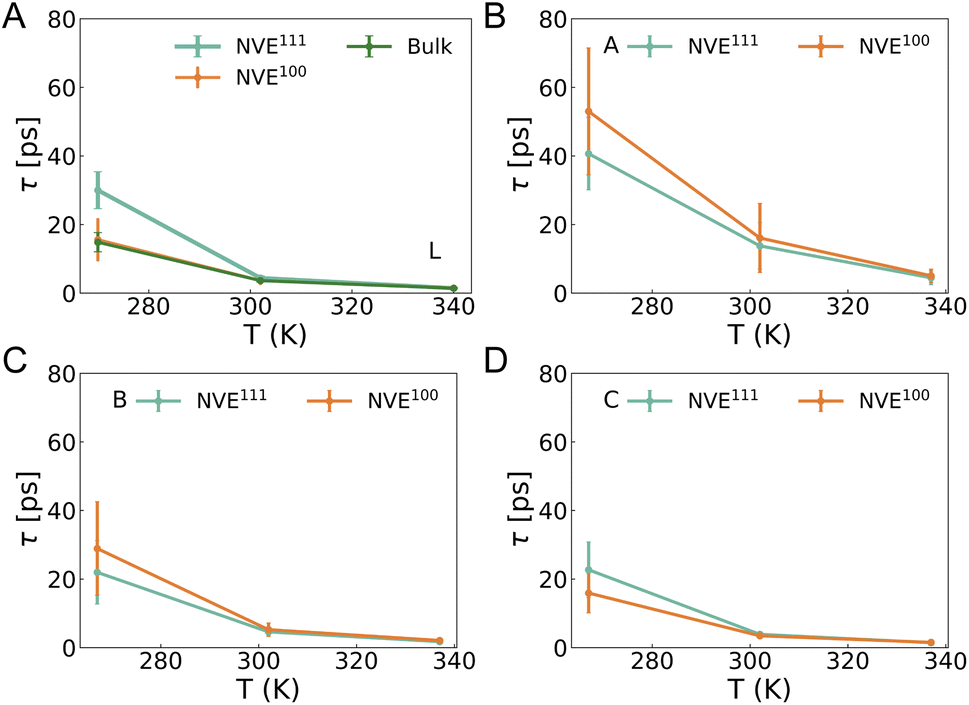Fig. 4 The fitted lifetime for water bisector reorientation dynamics. Here only the slow lifetimes are shown. See Fig. S13† for the fast lifetimes. (A) Water L at Pt(100)/water and Pt(111)/water interfaces and pure bulk water molecules (green). (B) Water A at the interfaces. (C) Water B at the interfaces. (D) Water C at the interfaces.

3.5 Water exchange dynamics and mechanism

Following a comprehensive benchmark comparison of the temperature-dependent dynamic properties with the experimentally observed dynamics of bulk water, a closer alignment was observed upon increasing the simulated temperature by 50 K. This adjustment will be considered in our investigation of water exchange dynamics.

To study the residence dynamics and avoid the inclusion of water molecules that are at the boundary of different adsorption peaks, we use the middle vertical distance between the peaks and valleys of the oxygen density profiles. Specifically, we designate the region 1.8 to 2.45 Å from the Pt surface as the stable adsorbed region for water A, and 2.9 to 3.75 Å for water B. The collective set of adsorbed water molecules is denoted as AB. Additionally, we define the non-adsorbed state as the region spanning 5.2 to 12.75 Å away from the Pt surface, which allows us to examine water exchange dynamics with the adsorbed state. This strategy is also used by Natarajan and Behler.⁵³ The aforementioned classification permits the investigation of both the residence time of all adsorbed water molecules and the residence time of individual water molecules within the adsorbed layer (Fig. 5A). This distribution encompasses all residence times of individual water molecules. Here, we denote the residence time of all adsorbed water molecules as R and the residence time of a single individual water molecule as RS (Table 1).

Fig. 5 (A) The distribution of the residence time for the individual water molecule. (B) The pair correlation function of water molecules. Here, the referenced oxygen atoms of water molecules are those just before desorption occurs. The observed O′ of water molecules are those at the same snapshot but desorb within 10 ps. (C) The water flux correlation function for water AB at 302/337 K for Pt(100) and Pt(111). (D) The slope of the flux correlation functions over time. (E) The schematic representation of the water exchange mechanism. For clarity, the vacant sites that can be occupied by the surrounding water molecules are not shown.

Table 1 The residence time for all the adsorbed water molecules and individual water molecules (τ_R for one exponential fit of water AB and water A and τ_RS for the individual water molecules AB). For the residence time of individual water molecules, the residence times of a single water molecule in the AB region were collected. This resulted in a distribution of residence times, as shown in Fig. 5A. A single exponential function was used to fit this distribution, yielding a characteristic time representing the average residence time of individual water molecules. Here, the temperatures have been adjusted based on the benchmark comparison of water dynamics

	Ensemble	T (K)	τ R (ps)		τ RS (ps)
			AB	A	AB
Pt(100)	NVT	302	208(19)	50(17)	74
		337	90(8)	18(8)	42
	NVE	302	224(16)	44(12)	79
		337	99(7)	20(4)	45
Pt(111)	NVT	302	240(20)	33(7)	112
		337	107(10)	13(3)	55
	NVE	302	251(21)	34(7)	128
		337	106(13)	13(3)	60

---

As shown in Table 1, the residence time for water A (τ_R) at 302/337 K is only on the order of tens of picoseconds for both interfaces, indicating that water molecules in the A region exhibit a high degree of flexibility and readily depart from the adsorbed layer. The timescales for water AB at 302/337 K are significantly faster than the residence times of adsorbed water molecules at Pt(100)/water and Pt(111)/water interfaces obtained from classical MD simulations⁶⁰ at 298 K (ranging from several to tens of nanoseconds)^17,19 with high water coverage (larger than 85%). To facilitate comparison with the previous MLMD study, we also fitted the lifetime of water AB using two exponential forms. At the Pt(111)/water interface, the slow residence time at 302 K (352 K without adjustment) in this work is approximately 20% (100 ps) faster than that obtained from previous MLMD simulations at 350 K for the same interface,⁶¹ which may be related to the model difference (the inclusion/exclusion of the liquid/vacuum interface, the cell size). It is difficult to definitively exclude the possibility of both timescales fitted using different exponential forms based solely on residence dynamics analysis. However, further analysis of the water flux correlation function, presented in the next section, indicates that exchange processes associated with the slower timescale extracted from two exponential forms cease much earlier. Therefore, we favor the timescale obtained from τ_R. If individual water molecules resided in the adsorbed layer independently, the overall residence time would be significantly longer than the residence time of individual water molecules. However, the observed ratio between the residence time of individual water molecules and the residence time (τ_R) of water AB is only 2–3. This suggests that when an individual water molecule departs from the adsorbed layer, its departure influences the residence times of other water molecules, effectively reducing the overall residence time of the adsorbed water molecules.

To investigate the spatial correlation of exchange events, we examined the RDF of adsorbed water molecules. The reference water molecule is the first to desorb, while the observed water molecules are those desorbing shortly after the initial event. We scrutinized the final snapshot just before the first desorption transpires, testing periods of 5/10 ps to ensure consistency (Fig. S14†). The results remained unaffected by the choice of period. Fig. 5B demonstrates that the RDF exhibits a peak at a pair distance of approximately 2.7 Å, corresponding predominantly to the first solvation shell of water molecules within the adsorbed layer. When an adsorbed water molecule breaks free from the solvation shell at the adsorbed layer, the original hydrogen bond network is broken. Consequently, the surrounding adsorbed water molecules are afforded a heightened likelihood of exchanging with non-adsorbed water. This spatial correlation gradually diminishes beyond 2.7 Å and becomes less pronounced at distances exceeding 10 Å.

To investigate the temporal correlation during the exchange process, we employed the flux correlation function as outlined in eqn (6) in the method section. The rapid exchange between water A and B (Fig. S15†) aligns with their respective residence times. The correlation results for the exchange between water AB and non-adsorbed water molecules are illustrated in Fig. 5C. Fig. 5D displays the slope of this flux correlation function over time, reflecting the rate of water exchange. When the exchange rate decays to zero, all adsorbed water molecules no longer reside in the adsorbed layer. Notably, the exchange rate demonstrates an initial increase within the first 5–10 ps, suggesting the efficacy of correlation at this timescale.

To provide a concise overview of the water exchange process, we propose a three-stage model based on the desorption of all initially adsorbed water molecules as shown in Fig. 5E.

Pre-desorption stage: prior to the initiation of the exchange process (Fig. S16B†), the hydrogen bond network evolves, and local adsorbed water molecules lose one or two hydrogen bonds (Fig. S16C†). This loss of hydrogen bonds results in faster instantaneous water diffusion (Fig. S16D†).

Acceleration stage: following the initiation of the first desorption event, the local hydrogen-bond environment is distorted, significantly increasing the likelihood of desorption for adjacent adsorbed water molecules. This distortion triggers a chain reaction of successive desorption events, driven by both spatial and temporal correlations. It is important to note that the relatively low coverage of A (0.15 ML) and AB (0.58/0.71 ML for Pt(111) and Pt(100)) means that space for incoming water molecules to adsorb is not a limiting factor, in contrast to classical MD simulations.¹⁹

Post-desorption stage: approximately 10 ps into this stage, a significant fraction of the initially adsorbed water molecules have transitioned to the bulk region. The remaining adsorbed water molecules are isolated within their new local hydrogen bond environments. This isolation results in a diminishing of spatial and temporal correlations, leading to a gradual decline in the exchange rate until it eventually halts.

4 Conclusions

In conclusion, we systematically investigated the water exchange dynamics at the Pt(100) and Pt(111) water interfaces using MLMD simulations. Increasing the MD temperature by approximately 50 ± 10 K aligned the PBE-D3 predictions of water dynamics with experimental observations of diffusion and reorientation dynamics. We determined that the timescales for water exchange dynamics are around several hundred picoseconds (tens of picoseconds for water exchange between A and B) at the experimental temperatures of 337/302 K. These timescales suggest that water exchange dynamics could influence reaction mechanisms, particularly when water molecules act as reacting species. We also found that water exchange is expedited by the correlation of desorption events, particularly within the first solvation shell of water molecules and during the first few picoseconds. This research provides valuable insights into the water exchange dynamics at solid/liquid interfaces.

Data availability

The machine learning potentials and Pt(111)/water and Pt(100)/water models are available at https://dataverse.ikkem.com/dataverse.xhtml.

Author contributions

F.-T. W., X. L. and J. C. designed the research; F.-T. W. and J.-X. Z. performed the research; F.-T. W., C. L., K. X., X. L. and J. C. analyzed the data; F.-T. W., J.-X. Z., C. L., K. X., X. L., and J. C. wrote the paper.

Conflicts of interest

The authors declare no conflict of interest.

Acknowledgements

F.-T. W. thanks Doctor Qi-Xin Chen for the helpful discussion. J. C. acknowledges the financial support provided by the National Natural Science Foundation of China (No. 22225302, 21991151, 21991150, 22021001, 92161113), the Fundamental Research Funds for the Central Universities (20720220009), and Laboratory of AI for Electrochemistry (AI4EC), IKKEM (Grant No. RD2023100101 and RD2022070501). X. Liu acknowledges the financial support provided by the National Natural Science Foundation of China (No. 42125202, 42421002).

Notes and references

1. Z. W. Seh, J. Kibsgaard, C. F. Dickens, I. Chorkendorff, J. K. Nørskov and T. F. Jaramillo, Science, 2017, 355, eaad4998.
2. H. Helmholtz, Ann. Phys., 1853, 165, 211–233.
3. H. Helmholtz, Ann. Phys., 1879, 243, 337–382.
4. D. L. Chapman, Philos. Mag., 1913, 25, 475–481.
5. O. Stern, Z. Elektrochem., 1924, 30, 508–516.
6. D. C. Grahame, Chem. Rev., 1947, 41, 441–501.
7. M. F. Toney, J. N. Howard, J. Richer, G. L. Borges, J. G. Gordon, O. R. Melroy, D. G. Wiesler, D. Yee and L. B. Sorensen, Nature, 1994, 368, 444–446.
8. J. J. Velasco-Velez, C. H. Wu, T. A. Pascal, L. F. Wan, J. Guo, D. Prendergast and M. Salmeron, Science, 2014, 346, 831–834.
9. C. Y. Li, J. B. Le, Y. H. Wang, S. Chen, Z. L. Yang, J. F. Li, J. Cheng and Z. Q. Tian, Nat. Mater., 2019, 18, 697–701.
10. F. Perakis, L. D. Marco, A. Shalit, F. Tang, Z. R. Kann, T. D. Kuhne, R. Torre, M. Bonn and Y. Nagata, Chem. Rev., 2016, 116, 7590–7607.
11. G. Zwaschka, Y. Tong, M. Wolf and R. Kramer Campen, ChemElectroChem, 2019, 6, 2675–2682.
12. F. Lapointe, M. Wolf, R. K. Campen and Y. Tong, J. Am. Chem. Soc., 2020, 142, 18619–18627.
13. G. Zwaschka, F. Lapointe, R. K. Campen and Y. Tong, Curr. Opin. Electrochem., 2021, 29, 100813.
14. E. Santos and W. Schmickler, Chem. Rev., 2022, 122, 10581–10598.
15. Y. C. Lam, A. V. Soudackov and S. Hammes-Schiffer, J. Phys. Chem. Lett., 2019, 10, 5312–5317.
16. R. E. Warburton, A. V. Soudackov and S. Hammes-Schiffer, Chem. Rev., 2022, 122, 10599–10650.
17. D. T. Limmer, A. P. Willard, P. Madden and D. Chandler, Proc. Natl. Acad. Sci. U. S. A., 2013, 110, 4200–4205.
18. A. P. Willard, D. T. Limmer, P. A. Madden and D. Chandler, J. Chem. Phys., 2013, 138, 184702.
19. D. T. Limmer, A. P. Willard, P. A. Madden and D. Chandler, J. Phys. Chem. C, 2015, 119, 24016–24024.
20. J. Le, M. Iannuzzi, A. Cuesta and J. Cheng, Phys. Rev. Lett., 2017, 119, 016801.
21. H. H. Kristoffersen, T. Vegge and H. A. Hansen, Chem. Sci., 2018, 9, 6912–6921.
22. S. Sakong and A. Gross, Phys. Chem. Chem. Phys., 2020, 22, 10431–10437.
23. S. Yoo, X. C. Zeng and S. S. Xantheas, J. Chem. Phys., 2009, 130, 221102.
24. T. Morawietz, A. Singraber, C. Dellago and J. Behler, Proc. Natl. Acad. Sci. U. S. A., 2016, 113, 8368–8373.
25. S. Du, S. Yoo and J. Li, Frontiers in Physics, 2017, 5, 34.
26. R. Halonen, I. Neefjes and B. Reischl, J. Chem. Phys., 2023, 158, 194301.
27. A. J. Page, T. Isomoto, J. M. Knaup, S. Irle and K. Morokuma, J. Chem. Theory Comput., 2012, 8, 4019–4028.
28. J. E. Basconi and M. R. Shirts, J. Chem. Theory Comput., 2013, 9, 2887–2899.
29. X. Y. Li, A. Chen, X. H. Yang, J. X. Zhu, J. B. Le and J. Cheng, J. Phys. Chem. Lett., 2021, 12, 7299–7304.
30. K. Yoshida, C. Wakai, N. Matubayasi and M. Nakahara, J. Chem. Phys., 2005, 123, 164506.
31. S. Woutersen, U. Emmerichs and H. J. Bakker, Science, 1997, 278, 658–660.
32. M. Praprotnik and D. Janezic, J. Chem. Phys., 2005, 122, 174103.
33. J. VandeVondele, M. Krack, F. Mohamed, M. Parrinello, T. Chassaing and J. Hutter, Comput. Phys. Commun., 2005, 167, 103–128.
34. S. Goedecker, M. Teter and J. Hutter, Phys. Rev. B:Condens. Matter Mater. Phys., 1996, 54, 1703–1710.
35. C. Hartwigsen, S. Goedecker and J. Hutter, Phys. Rev. B:Condens. Matter Mater. Phys., 1998, 58, 3641–3662.
36. J. VandeVondele and J. Hutter, J. Chem. Phys., 2007, 127, 114105.
37. J. P. Perdew, K. Burke and M. Ernzerhof, Phys. Rev. Lett., 1996, 77, 3865–3868.
38. S. Grimme, J. Antony, S. Ehrlich and H. Krieg, J. Chem. Phys., 2010, 132, 154104.
39. Y. Zhang, H. Wang, W. Chen, J. Zeng, L. Zhang, H. Wang and W. E, Comput. Phys. Commun., 2020, 253, 107206.
40. L. Zhang, J. Han, H. Wang, R. Car and W. E, Phys. Rev. Lett., 2018, 120, 143001.
41. S. Plimpton, J. Comput. Phys., 1995, 117, 1–19.
42. S. Nosé, J. Chem. Phys., 1984, 81, 511–519.
43. W. G. Hoover, Phys. Rev. A, 1985, 31, 1695–1697.
44. J.-X. Zhu, J.-B. Le, M. T. M. Koper, K. Doblhoff-Dier and J. Cheng, J. Phys. Chem. C, 2021, 125, 21571–21579.
45. I.-C. Yeh and G. Hummer, J. Phys. Chem. B, 2004, 108, 15873–15879.
46. B. Dünweg and K. Kremer, J. Chem. Phys., 1993, 99, 6983–6997.
47. C. Rønne, P.-O. Åstrand and S. R. Keiding, Phys. Rev. Lett., 1999, 82, 2888–2891.
48. T. A. Pham, T. Ogitsu, E. Y. Lau and E. Schwegler, J. Chem. Phys., 2016, 145, 154501.
49. M. V. Fernández-Serra and E. Artacho, J. Chem. Phys., 2004, 121, 11136–11144.
50. J. VandeVondele, F. Mohamed, M. Krack, J. Hutter, M. Sprik and M. Parrinello, J. Chem. Phys., 2004, 122, 014515.
51. L.-M. Liu, M. Krack and A. Michaelides, J. Chem. Phys., 2009, 130, 234702.
52. F.-T. Wang, X. Liu and J. Cheng, Mater. Futures, 2024, 3, 041001.
53. S. K. Natarajan and J. Behler, Phys. Chem. Chem. Phys., 2016, 18, 28704–28725.
54. J. Liu, X. He, J. Z. H. Zhang and L. W. Qi, Chem. Sci., 2018, 9, 2065–2073.
55. Y. Ding, A. A. Hassanali and M. Parrinello, Proc. Natl. Acad. Sci. U. S. A., 2014, 111, 3310–3315.
56. M. Ceriotti, J. Cuny, M. Parrinello and D. E. Manolopoulos, Proc. Natl. Acad. Sci. U. S. A., 2013, 110, 15591–15596.
57. M. J. Gillan, D. Alfe and A. Michaelides, J. Chem. Phys., 2016, 144, 130901.
58. A. K. Soper, ISRN Phys. Chem., 2013, 2013, 1–67.
59. D. Laage and J. T. Hynes, Science, 2006, 311, 832–835.
60. J. I. Siepmann and M. Sprik, J. Chem. Phys., 1995, 102, 511–524.
61. A. E. Mikkelsen, J. Schiøtz, T. Vegge and K. W. Jacobsen, J. Chem. Phys., 2021, 155, 224701.

---

Footnotes

† Electronic supplementary information (ESI) available. See DOI: https://doi.org/10.1039/d4sc06967f

‡ These authors contributed equally to this work.

---