DOI:
10.1039/D4NR03812F
(Paper)
Nanoscale, 2025,
17, 7114-7127
Kinetic analysis of silver nanowire synthesis: polyol batch and continuous millifluidic methods†
Received
17th September 2024
, Accepted 25th January 2025
First published on 27th January 2025
Abstract
This study investigates the variation in rate constants for nucleation and growth of silver nanowires (AgNWs) synthesized using the polyol method in batch and millifluidic flow reactors (MFRs). In a particular reactor, silver ion concentration at any time is quantified by the method of El-Ghamry et al. and the non-linear two-step Finke–Watzky model is used to determine the rate constants for nucleation (k1) and growth (k2). The results indicate that k1 and k2 for the MFRs are approximately four and two times larger, respectively, than the batch reactor rate constants. Additionally, the concentration, yield, and diameter of the synthesized AgNWs were determined using ultraviolet-visible (UV-vis) spectroscopy data. The results indicated that the concentration and yield of AgNWs synthesized using the MFR were approximately 10 times higher than those obtained with the batch reactor. Overall, AgNW synthesis in MFRs is about three times faster than the batch reactor. The coiled configuration of the MFRs promotes AgNW growth, minimizes temperature transients, and enhances reagent mixing caused by Dean vortices. This study highlights the potential of MFRs for the continuous synthesis of AgNWs and provides insights into the underlying growth mechanism.
 Shohreh Hemmati | Dr Shohreh Hemmati is an Assistant Professor of Chemistry at University of Southern Mississippi (USM). Prior to this position, she served as an Assistant Professor of Chemical Engineering at Oklahoma State University (OSU) from 2018 to 2024. Before joining OSU, she was a Postdoctoral Researcher at Purdue University. Dr Hemmati earned her Ph.D. in Chemical Engineering from the University of New Hampshire in 2016. She holds an M.S. in Energy Engineering from Sharif University of Technology, where she also worked as a Research Scientist at the Sharif Energy Research Institute from 2009 to 2012. Dr Hemmati received her B.S. in Chemical Engineering from Arak University in 2006. Dr Hemmati's research interests focus on green nanotechnology and nanomanufacturing. Specifically, she specializes in the synthesis of metal nanostructures, with an emphasis on green and sustainable methods using millifluidic techniques. She integrates these techniques with machine learning to achieve precise control over the size and morphology of the nanostructures. Dr Hemmati's research is primarily funded by the National Science Foundation (NSF). |
1. Introduction
Currently, transparent conductive film (TCF) technology uses n-type indium tin oxide (ITO) applied to substrates via vacuum deposition techniques such as physical vapor deposition. The relative scarcity and high cost of indium, a key component in ITO, has prompted investigation into nanomaterials for the next generation of flexible, low-cost TCFs.1 Non-ITO TCFs are being manufactured with metal grids, conductive polymers, graphene, and various one-dimensional (1D) nanostructures.2 AgNWs are a relatively cost-effective conductive material, especially compared to traditional materials like ITO, while also offering high electrical conductivity and mechanical flexibility. AgNW based TCFs are currently used in many applications like touch screens,3,4 solar cells,5 electromagnetic shielding,6 and sensors.7,8 The stretchability, bending performance, electrical conductivity, and optical transparency of AgNW TCFs depend on dimensional homogeneity and aspect ratio (ratio of length to diameter) of the nanowire structures, which are primary considerations for AgNW synthesis. AgNWs with high aspect ratios and dimensional homogeneity are commonly synthesized via template methods and wet chemical methods.1 AgNW template synthesis involves growing Ag nanoclusters onto a prepared 1D template. Template methods fall into two different categories, “soft” and “hard” based on the nature of the template.9 In hard template AgNW syntheses, the size and morphology can be easily controlled, but the purification and separation methods are more difficult. Soft template AgNW syntheses are easier to purify and separate because the templates dissolve in solution. Disadvantages of soft template AgNW syntheses include AgNW production with low aspect ratios, polycrystallinity, low yield per reaction, and irregular morphologies.10 Wet chemical methods offer solutions to the issues associated with template methods because they can achieve high purity AgNWs by adjusting chemical reaction parameters.1
AgNW synthesis by the polyol method is widely regarded as a relatively simple and dependable approach, often cited for its cost-effectiveness under laboratory-scale conditions. This low-temperature reaction produces the desired morphology at high yield.1 The polyol method uses a glycol solvent and reducing agent to ionize silver nitrate and to reduce the silver ion (Ag+) to Ag0. A capping agent is used to cover the {100} facets of Ag crystal seeds to promote 1D growth. A salt mediator scavenges oxygen and aids in the slow release of Ag+ into solution from a silver salt metal precursor.11
Batch reactors, commonly used for polyol AgNW syntheses, face limitations for mass production. While batch reactors can efficiently produce silver nanoparticles (AgNPs) with controlled morphology, size, and selectivity, successful production of AgNWs with controlled morphology, size, and selectivity is more difficult. Other issues with AgNW syntheses in batch reactors include batch-to-batch variability and non-linear scaling of mass and heat transfer properties with reactor volume due to domination by convective forces in a turbulent environment rather than diffusion in laminar flow.12 The dimensionless Reynolds (Re) number is used to determine the flow region in reactor vessels and tubing as shown in eqn (1).
| |  | (1) |
Where
ρ is fluid density,

is fluid speed,
d is inner reactor diameter, and
µ is dynamic viscosity of the fluid. While batch reactors ensure proper mixing, the chaotic nature of the turbulent environment disrupts AgNW formation. Continuous flow reactors (CFRs) can easily be designed in the laminar flow regime (Re < 2000) where diffusive mass transfer and conductive heat transfer dominate.
CFRs operate at relatively low volumetric flowrates, are constructed from various tubing materials, and possess a 0.1 to 10 mm inner tubing diameter. Heat transfer to the reactants inside the tubing from an external heat bath occurs by conduction through the tube wall, where conduction refers to the transfer of heat via molecular collisions within a material, and across the diameter of the flowing reactants, which involves a combination of conduction and convection. The heat transfer is characterized by the Nusselt (Nu) number. MFRs are advantageous over microfluidic flow reactors due to ease of fabrication and the larger channel size allowing for higher flowrates, lower inlet pressures, and larger throughput whilst maintaining laminar flow conditions. Additionally, the orders of magnitude larger channel size allow for AgNWs to easily be synthesized without clogging the tubing. In the early 1920s, Dean investigated flow characteristics in coiled tubing, and discovered that a pair of symmetric vortices (DVs) formed on the cross-sectional plane of the tubing due to centrifugal forces as illustrated in Fig. 1.13–15 He characterized the strength of these secondary flow patterns using the Dean (De) number as shown in eqn (2).
| |  | (2) |
Where
d is the channel diameter and
D is the diameter of the coil.
12
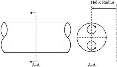 |
| | Fig. 1 Illustration of DVs transverse to primary flow in coiled tubular reactors. | |
A larger De indicates a stronger effect of DVs. Kumar et al.16 demonstrated a significant enhancement in mixing efficiency at Re ≈ 10 by analyzing concentration distributions and unmixed coefficients across different cross-sections and process conditions in curved tube flow reactors, as compared to straight tube flow reactors. Their findings highlight the superior mixing capabilities of curved tube reactors under various operational conditions.17,18 MFRs can be configured in many ways but are commonly coiled to increase reagent mixing efficiency caused by DVs and mitigate boundary layer stagnation at the wall of the tubing.12
Several researchers have experimentally determined reaction rate constants and activation energies for polyol synthesis in batch reactors using timed sampling and Ultraviolet-visible (UV-vis) spectroscopy. Dong et al. synthesized AgNP using the Turkevich method in a batch reactor. The authors adjusted the reduction rate by varying the pH of the reaction solution and determined the rate constants using a spectrophotometric method. Reaction solution was sampled and analyzed using UV-vis spectroscopy at differing reaction times for each pH range.19 Wang et al. performed a kinetic study on the polyol synthesis of Pd nanocrystals in a batch reactor by taking reaction samples and characterizing them using UV-vis throughout the reaction. The authors used the spectra for the PdCl42− ion that has visible peaks at 222 and 279 nm to determine the rate constant, activation energy, and initial rate of the polyol reaction.20 Patil et al. conducted a kinetic study of the polyol synthesis of AgNWs in a batch reactor. The authors used ethylene glycol (EG), silver nitrate (AgNO3), polyvinylpyrrolidone (PVP), and iron(III) chloride (FeCl3) as the solvent/reducing agent, metal precursor, capping agent, and salt mediator, respectively. A redox-crystallization model was used to quantify the rate constants for nucleation (k1) and growth (k2) at 150 °C in an open batch reactor. Rate constants for k1 and k2 were determined to be 1 × 10⁻⁵ s−1 and 5 × 10⁻³ s−1, respectively.21
This study focuses on quantifying the nucleation and growth rate constants of the polyol synthesis of AgNWs in both batch and MFRs. To quantify the polyol reaction kinetics, [Ag+] was calculated at different residence times by submerging corresponding lengths of reaction tubing in a thermostatic oil bath and then quenching reaction samples from the MFR. Linear and nonlinear two-step Finke–Watzky models for AgNP formation were used to calculate and compare the nucleation and growth rate constants for each model and reactor.22
The superior production capacity of MFRs offers substantial promise for large-scale applications in industry. However, scaling up MFR systems for industrial production poses challenges, including maintaining uniform flow and effective heat and mass transfer. Solutions, such as reactor parallelization or modular system designs, could address these challenges, but further investigation is essential to optimize these approaches for industrial settings.
2. Experimental
2.1. Materials
The batch reactor assembly consisted of a 250 mL three neck, round bottom glass flask, a glass reflux condenser, glass stoppers, 12.5 mm magnetic stirring bar, a hot plate, temperature controller, and glass dish filled with sufficient silicone oil. The MFR assembly required a syringe pump, plastic syringes, 1.5 mm inner diameter (ID) polytetrafluoroethylene (PTFE) tubing, 1.6 mm ID polypropylene t-joint connectors, a hot plate, a temperature controller, a 40 mm magnetic stirring bar, a glass dish with sufficient silicone oil, and a Falcon tube collection flask. The kinetic study required 1.5 mL methacrylate cuvettes (Fisher Scientific, 14-955-128).
Silicone oil (Fisher, 200553), Copper(II) Chloride (CuCl2, Sigma-Aldrich, 203149, 99%), polyvinylpyrrolidone (PVP, Sigma-Aldrich, 856568, Avg. MW: 55![[thin space (1/6-em)]](https://www.rsc.org/images/entities/char_2009.gif) 000), silver nitrate (AgNO3, Sigma-Aldrich, 209139, ≥99%), ethylene glycol (EG anhydrous, Sigma-Aldrich, 324558, 99.8%), and acetone (C3H6O, Honeywell, 10626710) were all purchased and used without further purification for the polyol AgNW synthesis in both batch and MFRs. The kinetic study required sodium acetate (C2H3NaO2, Sigma-Aldrich, S2889), 2,4,5,7-tetrabromofluorescein (C20H8Br4O5, Sigma-Aldrich, E4009), 1,10 phenanothroline (C12H8N2, Sigma-Aldrich, 131377), ethyl alcohol (C2H5OH, Sigma-Aldrich, 459836, 100%), and glacial acetic acid (CH3CO2H, Sigma-Aldrich, 64-19-7) that were all purchased and used without further purification to quantify Ag+ in reaction solution.
000), silver nitrate (AgNO3, Sigma-Aldrich, 209139, ≥99%), ethylene glycol (EG anhydrous, Sigma-Aldrich, 324558, 99.8%), and acetone (C3H6O, Honeywell, 10626710) were all purchased and used without further purification for the polyol AgNW synthesis in both batch and MFRs. The kinetic study required sodium acetate (C2H3NaO2, Sigma-Aldrich, S2889), 2,4,5,7-tetrabromofluorescein (C20H8Br4O5, Sigma-Aldrich, E4009), 1,10 phenanothroline (C12H8N2, Sigma-Aldrich, 131377), ethyl alcohol (C2H5OH, Sigma-Aldrich, 459836, 100%), and glacial acetic acid (CH3CO2H, Sigma-Aldrich, 64-19-7) that were all purchased and used without further purification to quantify Ag+ in reaction solution.
2.2. Methods
2.2.1. Batch AgNW synthesis.
The round bottom flask, fitted with a stir bar, was equipped with a reflux condenser in the center neck, while the other two necks were sealed with glass stoppers, as depicted in Fig. 2.15 The flask was heated in a silicone oil bath to the reaction temperature of 158 °C for 10 minutes. Next, 15 mL of EG was pipetted into the flask and stirred at 300 RPM for 60 minutes. The initial reagent concentrations were [AgNO3] = 0.102 M, [PVP] = 0.124 M, and [CuCl2] = 5.16 mM. All reactants were prepared in 4.5 mL of EG. All solutions were mixed till homogeneous, while the silver nitrate solution was sonicated for 6 minutes.23 After the EG was heated for 60 minutes, 120 µL of CuCl2 was pipetted into the round bottom flask, and the mixture was heated for an additional 15 minutes while maintaining stirring. Next, 4.5 mL of the PVP solution was pipetted into the round bottom flask. The final step was to add 4.5 mL of the AgNO3 solution, approximately 1 drop per second, into the reaction flask and allow the reaction to proceed for 90 minutes. Every 10 minutes, 200 μL of the reaction solution was collected via pipette and then diluted in deionized (DI) water to await measurement of the remaining Ag+ in the reaction solution using UV-vis spectroscopy. A total of 2 mL was removed over a 90 minute time interval, and it is assumed that the gradual reduction in reagent volume does not have significant impact on mass or heat transfer properties. To prepare for scanning electron microscope (SEM) characterization of the synthesized AgNWs and Ag nanostructures, samples were washed and centrifuged for 30 minutes at 3000 RPM once with acetone, twice more with DI water, and then stored in DI water.23
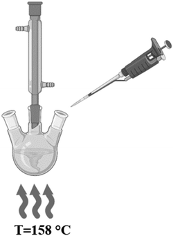 |
| | Fig. 2 Schematic of the batch reactor setup for the polyol AgNW synthesis. | |
2.2.2. MFR AgNW synthesis.
To maintain a constant flowrate of 40 µL min−1, sections of 1.5 mm ID PTFE tubing were cut and coiled to maintain a 6-inch (152 mm) helix diameter. The tubing bundles were then submerged and suspended using fixation wires in a well-stirred, silicone oil bath heated to the reaction temperature of 158 °C, as illustrated in Fig. 3.15 The calculated lengths of tubing for each residence time are shown in Table 1. To analyze the results and effects of maintaining a constant tubing length while varying flowrates, the calculated flowrates, corresponding dimensionless numbers, and heat transfer coefficients are provided in Table S1 in the ESI.† AgNO3 and PVP reagent solutions were prepared in 50 mL of EG, while copper chloride was prepared in 4.5 mL of EG.
 |
| | Fig. 3 Schematic of the MFR configuration for the polyol AgNW synthesis. | |
Table 1 Millifluidic reactor tubing lengths for the corresponding residence time
| Residence time (min) |
Tubing length (in) |
| 4 |
3.6 |
| 8 |
7.1 |
| 12 |
10.7 |
| 16 |
14.3 |
| 20 |
17.8 |
| 24 |
21.4 |
| 28 |
25.0 |
| 32 |
28.5 |
| 36 |
32.1 |
| 40 |
35.6 |
The concentration of the reagents were [AgNO3] = 0.102 M, [PVP] = 0.124 M, and [CuCl2] = 5.16 mM, and all solutions were mixed till homogeneous. The silver nitrate solution was sonicated for 6 minutes.24 After the reagent solutions were prepared, 667 µL of the CuCl2 solution was mixed into both AgNO3 and PVP solutions. For each residence time, 5 mL of the reagent solutions were loaded into a 5 mL plastic syringe and then connected to the PTFE tubing as seen in Fig. 3.
The samples were collected in a Falcon tube for further characterization. Ag+ and AgNWs were prepared for UV-vis by being diluted and stored in DI water. Reaction solutions were also prepared for SEM characterization by washing and centrifuging, once with acetone and then twice more with DI water, before storage in DI water.23,24 In each wash cycle, the supernatant was removed after centrifugation and the visible sediment retained for further washing.
2.2.3. Kinetic study.
A method by El-Gamry et al. was used to quantify the [Ag+] in reaction solution for a chosen residence time. The authors found that combining a Ag+ solution with a 1,10 phenanothroline (Phen)/2,4,5,7-tetrabromofluorescein (TBF) solution formed ternary Ag/Phen/TBF complexes detectable by UV-vis at 550 nm. Optimum pH and time were determined while the authors tested 33 different ions that could interfere with Ag forming the complex in the Phen/TBF mixture. It was found that the optimum pH range for the solution was between 4 to 8, the reaction proceeds immediately in the presence of Ag+, and there are only two potential ions, iridium(IV) and cyanide, that could interfere with Ag forming the complex. To evaluate the appropriate molar ratios for the Ag/Phen/TBF solution, the authors used Job's Plots and found the optimal molar ratio to form the Ag/Phen/TBF complex to be 2:4:1, respectively.25
A calibration curve was constructed to measure [Ag+] in a reaction solution for any residence time. Solutions of AgNO3 with known concentrations ranging from 0.01 to 0.1 mM were prepared in EG and a Phen/TBF buffer solution was prepared by combining 18 mL of an acetate buffer with 1 mL each of Phen and TBF solutions. The acetate buffer was prepared by dissolving 0.25 g of sodium acetate in 40 mL of DI water and then adding 54 µL of acetic acid. Solutions of 4.5 mM Phen and 1.5 mM TBF were prepared by dissolving the reagents in 100% pure ethyl alcohol. The pH of all the Phen/TBF solutions were measured to verify the pH was less than 8 but more than 4, and the Phen/TBF solutions were mixed using a stir plate until translucent bright pink.26 For the calibration curve measurements, a blank was prepared by combining 0.5 mL of DI water with 0.5 mL of the Phen/TBF solution in a 1.5 mL cuvette. After measuring the blank, a sample was prepared and measured by combining 0.5 mL of a known AgNO3 concentration solution with 0.5 mL of the Phen/TBF solution in a cuvette and then immediately placing the cuvette in the UV-vis spectrophotometer.
Data collection for both batch and the MFRs was conducted in the same manner. A reaction sample at a given time interval was collected from the reactor, diluted in DI water, and then 0.5 mL of the diluted sample was pipetted into a 1.5 mL cuvette. A blank was prepared by combining 0.5 mL of the Phen/TBF solution with 0.5 mL of deionized (DI) water in a 1.5 mL cuvette. After the blank was measured, 0.5 mL of the Phen/TBF solution was pipetted into the cuvette containing 0.5 mL of the sample and then immediately placed in the UV-vis spectrophotometer. Three measurements were taken at each time interval, and since AgNWs are detectable by UV-vis, an additional measurement was taken to subtract the AgNW spectra away from the ternary complex spectra before recording the absorbance value to calculate the [Ag+]. For these measurements, 0.5 mL of DI water was pipetted into a cuvette containing 0.5 mL of the diluted reaction sample and a DI water blank was used for the measurements. To investigate the total residence time for the MFR, a “length” study was conducted for residence times from 20 to 90 minutes. SEM images and ImageJ software were used to characterize and measure the wires length and diameter. The lengths, diameters, and aspect ratios were calculated and recorded for the selected residence time.
2.3. Characterization
2.3.1. AgNWs.
SEM (FEI Quanta 600 field-emission gun with Bruker EDS X-ray microanalysis system and HKL EBSD system) at the Oklahoma State University Microscopy Lab was used to characterize the samples at selected time intervals as well as the final synthesized AgNWs for both batch and millifluidic reactions. To prepare the samples for SEM, the samples stored in DI water were sonicated to fully disperse the AgNWs. After sonication, the suspensions were diluted and pipetted onto carbon tabs adhered to aluminum pins. The samples were dried for 24 hours under ambient conditions.
2.3.2. Batch reaction temperature profile.
The batch polyol AgNW temperature profile measurements were obtained using a React IR 700 TE MCT Detector with a DiComp (diamond) tip.
2.3.3. pH measurements.
All pH measurements were taken with a Thermo Scientific Orion Star A211 pH meter and Orion 8102BNUWP probe.
2.3.4. Absorbance measurements.
All absorbance values recorded to calculate the [Ag+] were measured using a Metler Toledo UV-vis UV5 spectrophotometer.
3. Results and discussion
3.1. Calibration curve
The color of the Ag/Phen/TBF solution corresponded to the number of ternary complexes formed and ranged from deep translucent pink (high [Ag+]) to light translucent pink (low [Ag+]).
Three measurements were taken for each known concentration and then plotted as seen in Fig. 4 where the error bars represent the range of measured absorbance.26
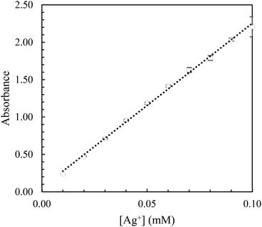 |
| | Fig. 4 Calibration curve used to calculate [Ag+] based on the absorbance measured at 550 nm. | |
A regression of the calibration data yields a linear relationship between [Ag+] (mM) and absorbance and is shown in eqn (3).
| | | [Ag+] = 21.964·absorbance + 0.0563 | (3) |
3.2. Experimental data
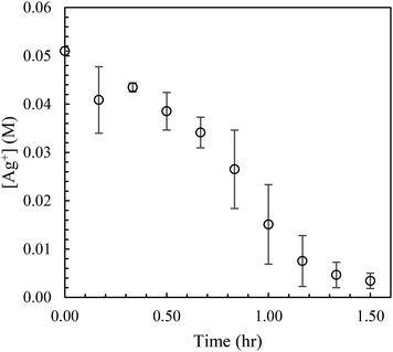
To obtain the Ag+ spectra for a given residence time, the AgNW spectra was subtracted from each of the three spectra taken, averaged, and then applied to eqn (3) to calculate the [Ag+]. The values were plotted against time as shown in Fig. 5 and 6 for batch and MFR, respectively.
 |
| | Fig. 5 The [Ag+] for the batch reactions calculated and plotted over time. | |
 |
| | Fig. 6 The [Ag+] for the MFR calculated and depicted over time. | |
The data collected to observe the effects of a constant tubing length is shown in Fig. S1 in ESI.† Data collection for the batch reactor spanned 1.5 hours, while for the millifluidic reactor, it spanned 0.67 hours.
Standard deviations of the data collected from the batch reactor varied from 0.9 to 8.2 mM, while the millifluidic data varied from 0.17 to 3.5 mM. The batch reactor required 70 minutes to reduce a majority of the Ag+ in solution, while the MFR required only 20 minutes to accomplish the same. It was found that the average length of the AgNWs varied by ±5 µm during minutes 30 through 90 of residence time. The average lengths, diameters, and aspect ratios were found to be 30 µm, 62 nm, and 490, respectively. Based on SEM images and the average lengths, it was determined that the necessary residence time for the millifluidic reactor is 30 minutes, which is one third the time required for the batch reaction.
3.3. SEM images
To characterize the samples at selected time intervals, SEM images were taken, as shown in Fig. 7 and 8, for batch and millifluidic reactors, respectively. In Fig. 7 (t = 10 min), nanoparticles are apparent as the bright white contrast objects with a gray halo and a dark background. Presumably, these nanoparticles are the result of nucleation and early growth of nanostructures occurring within the first 10 minutes of the reaction. Anisotropic growth in the [111] direction is observed around 50 minutes of reaction time in Fig. 7 (t = 50 min). Note that only a few nanoparticles at t = 50 min have transitioned to anisotropic growth. AgNW growth and AgNP formation continue through 90 minutes of reaction time as seen in Fig. 7 (t = 90).
 |
| | Fig. 7 SEM images taken at six different reaction times in the batch reactor. Nucleation begins at t = 10 min, AgNWs are beginning to form at t = 40 min, and the wires continue growing from t = 50 min through t = 90 min. (Scale bars: 5 μm). | |
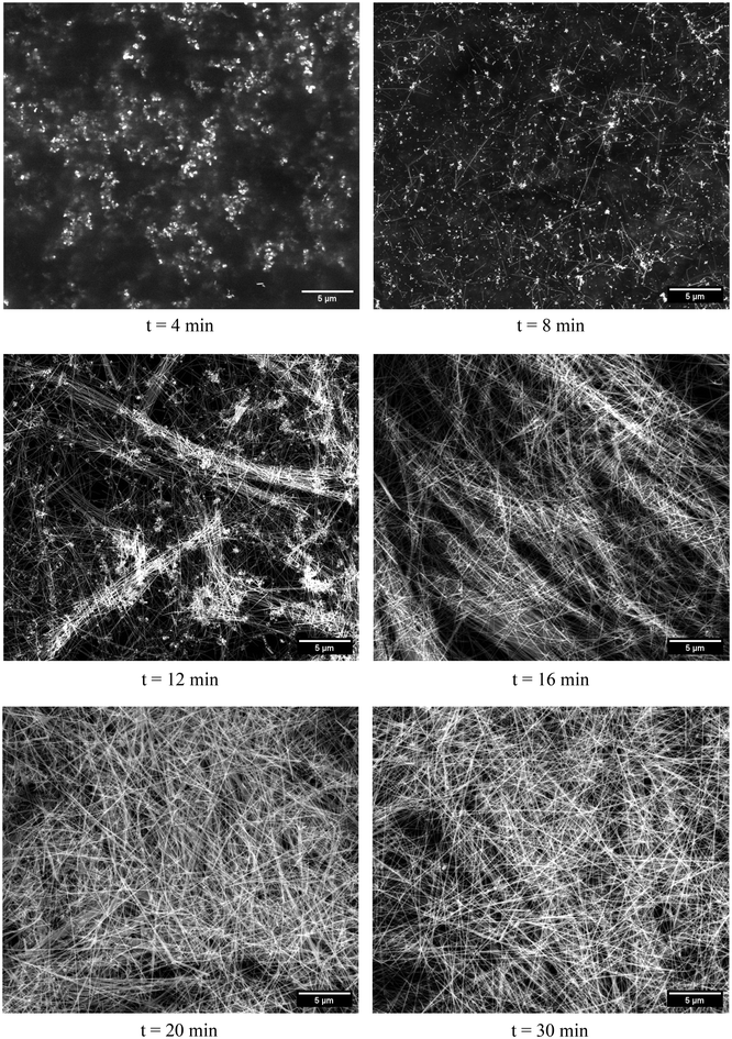 |
| | Fig. 8 SEM images taken at six different residence times in the millifluidic reactor. Nucleation occurs at t = 4 min, AgNWs are beginning to form at t = 8 min, and the wires continue to grow from t = 12 min through t = 30 min. (Scale Bars: 5 μm). | |
In the millifluidic reactor, nucleation occurs within the first 4 minutes of residence time and continues until 12 minutes as shown in Fig. 8 (t = 4, 8, & 12 min). In comparison to the batch reactor, the density of nuclei in the millifluidic reactor appears to be larger. The anisotropic growth of AgNWs in the [111] direction is observed around 8 minutes of residence time and continues until 30 minutes as shown in Fig. 8 (t = 16, 20 & 30 min).
Several observations about the SEM images for the batch and millifluidic reactors are apparent. First, nucleation time (t*) and the attendant nanoparticles that evolve first in either reactor, are both quicker to appear and at higher density in the MFR compared to the batch reactor. Second, the appearance of wire-like structures for the MFR occurs at t ≤ 2t* whereas it occurs at t ≤ 5t* in the batch reactor. Third, the yield of MFR is nearly 100% AgNWs whereas about 75% of the structures from the t = 90 min sample are AgNWs in batch reactor. Finally, the thickness, length and uniformity of AgNWs are thinner, longer, and more consistent in the MFR product compared to the batch reactor product.
3.4. Modeling
The Finke–Watzky two-step mechanism for modeling AgNP syntheses22,27 has been applied to the batch and millifluidic polyol syntheses of AgNWs. In this model it was assumed that in the first step, there is a pseudo first-order reaction between glycolaldehyde (GA) and Ag+. GA, produced while heating EG, reduces the Ag+ into Ag atoms (Ag0), as seen in eqn (4).| |  | (4) |
Where A is the initial concentration of silver ions (Ag+0), B is the concentration of silver atom (Ag0), and k1 is the rate constant for nucleation. After the pseudo first-order step, an autocatalytic growth of Ag0 and formation of Ag0 is assumed as the second step as seen in eqn (5).| |  | (5) |
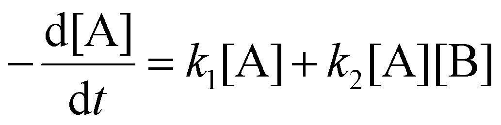
Where k2 is the rate constant for growth. The consumption rate of [A] can be derived from eqn (4) and (5) as shown in eqn (6).
| |  | (6) |
Where [A] is [Ag
+], [B] is [Ag
0],
k1 is the rate constant for nucleation, and
k2 is the rate constant for growth at any time,
t. To put variables into terms of [A], the [B] term can be expressed as the difference between [Ag
+]
0 and [Ag
+] at any time,
t, as seen in
eqn (7).
Substituting eqn (7) into eqn (6) gives eqn (8).
| |  | (8) |
Integrating eqn (8) while considering the initial conditions at t = 0, [Ag+]0 = [Ag+], and then algebraically rearranging for [A] gives eqn (9).
| | 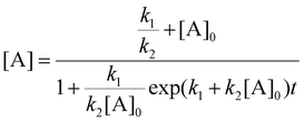 | (9) |
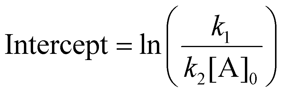
To linearize eqn (9), it was assumed that [A]0 > [A] and k2[A] ≫ k1 as seen in eqn (10).
| |  | (10) |
To perform the linear regression, the y-term from eqn (10) was used to calculate y-values for each time interval (t), as seen in eqn (11).
| | 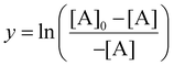 | (11) |
Where [A]
0 is [Ag
+]
0 and [A] is [Ag
+] at the time
t. The calculated
y-values were plotted against time for both batch and MFR experimental data as shown in Fig. S2 and S3,
† respectively; Fig. S4
† analyzes the
y-values depicted against time for the data considering a constant tubing length. Excel was used to obtain a line of best fit to calculate the slope and
y-intercept to quantify the nucleation and growth rate constants,
k1 (hr
−1) and
k2 (hr
−1 M
−1), using
eqn (12) and (13), respectively.
| |  | (13) |
The linear model for batch and MFRs failed to fit the experimental data accurately as seen in Fig. S5–S7 in the ESI.† The first assumption of the linear model, [A]0 > [A], does not accurately account for concentration changes occurring at the beginning of the reaction where [A]0 and [A] are equal or almost equal. Near the end of the reaction, the model appears to match the experimental data more accurately where the first assumption is more applicable. For the second assumption of the linear model, k2[A] ≫ k1, the dependence on [A] causes the entire term to approach zero as the concentration of Ag+ decreases in solution. In this case, the k1 and k2 terms are almost equal. For these reasons, only the nonlinear model results are shown below, while all linear model results are presented in the ESI.†
To perform the non-linear regression, eqn (9) was used to calculate [Ag+] using an initial guess for the rate constants, k1 and k2, for each time interval. The Solver function in Excel was used to minimize the sum of squared errors (SSE) of the initial guesses by adjusting the k1 and k2 values. The final values for k1 and k2 were found to be 0.18 h−1 and 71.9 h−1 M−1 for batch, and 0.79 h−1 and 158.3 h−1 M−1 for MFRs, respectively. Calculated values for [Ag+], obtained using the final k1 and k2 values, were plotted against time as illustrated in Fig. 9 and 10 for batch and MFRs, respectively. An SSE value was calculated for the non-linear Finke–Watzky model to be 7.9 × 10⁻⁵ and 3.8 × 10⁻⁴ for batch and MFRs, respectively. Rate constants were used to calculate [Ag+] for a constant tubing length and were plotted over time as shown in Fig. S8 in the ESI.† A summary of the results for batch and MFRs are shown in Table 2 for the non-linear Finke–Watzky model. Table S2 shown in the ESI† summarizes all results.
 |
| | Fig. 9 Non-linear fit of experimental [Ag+] as a function of reaction time in the batch reactor. | |
 |
| | Fig. 10 Non-linear fit of experimental [Ag+] as a function of residence time in the MFR. | |
Table 2 Nucleation (k1) and growth (k2) rate constants for batch and millifluidic reactors and the corresponding SSE
| Reactor |
Non-linear model |
|
k
1, hr−1 |
k
2, hr−1M−1 |
SSE |
| Batch |
0.18 |
71.9 |
7.9 × 10⁻⁵ |
| MFR |
0.79 |
158.3 |
3.8 × 10⁻⁴ |
The nonlinear model accurately modeled the trend and magnitude of [Ag+] concentration as a function of time for both batch and millifluidic reactors. Additionally, it was found that the growth rate constant (k2) for the MFR was approximately four times larger than the batch growth rate constant. The MFR could synthesize AgNWs in one-third of the batch reaction time.
The Damköhler (Da) number is a dimensionless number that describes the ratio of reaction rate to mass transfer rate in a reactor. When the Da > 1, the system is considered mixing-limited and could result in low or poor AgNW yield, but when the Da < 1, the system is considered kinetically reaction-limited where mixing is sufficiently fast.12 For a second order, irreversible reaction, the Da can be calculated using eqn (14).28
Where
τ is space time,
k2 is growth rate constant, and
CA0 is the initial concentration. Considering the MFR set up used in this study at standard reaction conditions with a tubing length corresponding to 30 min of residence time, the Da is equal to 0.02. This low value indicates that mixing is sufficiently fast, and that the system is kinetically limited.
3.5. Temperature profiles
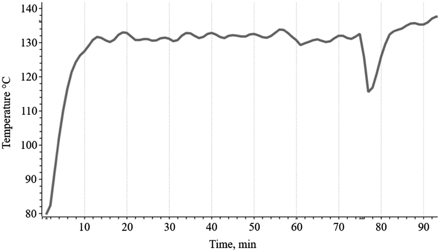
To further explore the differences in reaction environments between batch and MFRs, temperature profiles for both reactors were obtained. For the batch reactor, the silicone oil bath is large and well stirred relative to the reaction fluid. Hence, it can be safely assumed that the oil bath acts as a constant temperature thermal reservoir and serves as a constant temperature boundary condition for the heat transfer circuit consisting of the oil bath in series with the glass flask and the stirred contents of reactants. Interior to the 100 mL round bottom flask, where a 7.9 mm diameter, 12.7 mm length stir bar rotates at 300 RPM, the Re is estimated to be 32200. Under turbulent flow conditions, a film layer develops at the wall of the reaction cylinder where speed is equal to zero due to the non-slip boundary condition at the wall. Energy from the silicone oil is transferred through the wall of the flask and through the film layer where it is then transferred to the bulk of the reaction solution. During batch syntheses, reaction volume and temperature drastically change as reagents are added to the reactor. When considering the temperature profile measured using in situ React IR as illustrated in Fig. 11 for the batch reactor, at t = 60 min and t = 75 min, temperature drops are shown as 120 µL of CuCl2 and 4.5 mL each of AgNO3 and PVP solutions were slowly added to the reaction flask. Following the reagent additions there were notable temperature drops coupled with warm up periods back to reaction temperature.
 |
| | Fig. 11 Temperature profile taken for the batch reactor using in situ react IR. | |
Analyzing the primary flow conditions at 40 µL min−1 for the MFR reveals a Re equal to 0.4 due to the low fluid speed and small inner channel diameter. The De calculated for the MFR is equal to 0.04, indicating weak DVs and predominantly laminar flow conditions. However, the low De also suggests that the reaction fluid is subjected to the secondary transverse flow (due to wall confinement) for a longer duration, resulting in thinner and longer AgNWs.18 To calculate the temperature profile at the inlet of the MFR, the heat transfer coefficient (h) for the system was calculated using eqn (15).
| |  | (15) |
Where
k is the thermal conductivity of EG,
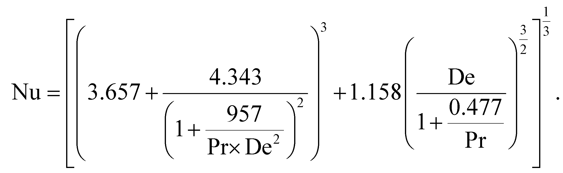
d is ID of reactor tubing, and Nu is the Nusselt dimensionless number for the system. To calculate the Nu, the Manlapaz–Churchill correlation for systems with De < 2000 was used as shown in
eqn (16).
| |  | (16) |
Where Pr and He are the Prandtl and Helical dimensionless numbers, respectively.
29,30 The Pr describes heat and momentum transport in a fluid system and was calculated to be 16.1 by using
eqn (17).
| |  | (17) |
Where
Cp is the heat capacity and
μ is the dynamic viscosity of EG.
Next, the He, which differs from the De by accounting for the effect of change in height on fluid flow through a coil, was calculated to be 0.04 by using eqn (18).
| |  | (18) |
Where
r is the inner radius of tubing and
Rc is the critical radius of the reactor tubing coil. The
Rc was calculated using
eqn (19).
| |  | (19) |
Where
R is the radius of the reactor tubing coil and
p is the pitch length between coils as depicted in
Fig. 12.
15
 |
| | Fig. 12 The radius of the reactor tubing, r, and the pitch (space between coils), p, is considered when calculating the critical radius for the He. | |
The reactor tubing used for this study was coiled and then bunched together, so it can be assumed that the length between the individual tubing coils is negligible (p = 0) which causes the Rc to equal the R of the tubing coil. Substituting in R for Rc allows He and De to be equivalent as seen in eqn (20).
| |  | (20) |
After substituting eqn (20) into eqn (19), eqn (21) was obtained.
| |  | (21) |
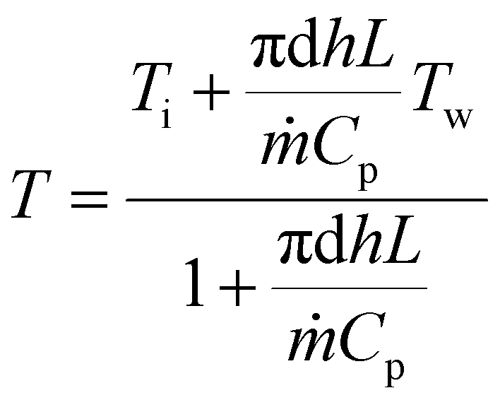
A Nu was calculated to be 3.90 by incorporating the values for Pr and De into eqn (21). The heat transfer coefficient (h) was calculated to be 725.2 W m−2 K−1 using eqn (15). Calculated values for the dimensionless numbers and the heat transfer coefficients for batch and MFRs are summarized in Table 3. MFRs perform at batch standards but can make AgNWs better in laminar flow. Finally, temperature, T, at any given tubing position (L) can be calculated for the MFR using eqn (22) obtained from an energy balance on the system.
| |  | (22) |
Where
Ti is the initial reaction solution temperature (20 °C),
Tw is the tubing wall temperature (158 °C), and
ṁ is mass flowrate (6.7 × 10
−7 kg s
−1). The temperature profile for the inlet of the MFR is shown in
Fig. 13.
 |
| | Fig. 13 The calculated temperature profile vs. position for the MFR. | |
Table 3 Calculated dimensionless numbers and heat transfer coefficient values for the MFR and batch reactors
| Number/property |
MFR value |
Batch value |
| Re |
0.40 |
32210 |
| De |
0.04 |
N/A |
| Pr |
16.1 |
16.1 |
| He |
0.04 |
N/A |
| Nu |
3.90 |
282 |
| Da |
0.04 |
0.01 |
|
h (W m−2 K−1) |
725.2 |
9585.0 |
Analyzing the temperature profile at the inlet of the MFR shows that adding small volumes of reagents (∼1 µL s−1) has a negligible effect on the average reaction solution temperature. Based on Fig. 13, the reaction solution travels approximately 0.5 mm out of 2 m of reaction tubing before reaching the reaction temperature (T = 158 °C). The small reaction volume of the tubing allows MFR reactions to maintain relatively constant average reaction temperature and experience much shorter reaction solution warm up times (Δt = 1.5 s) compared to the batch reactor (Δt = 10 min) after reagent addition.
3.6. Comparing diameter, concentration, and yield
To further compare the batch and MFR systems, additional information was obtained from the UV-vis spectra. The method described by Azani et al. was applied to calculate the absorption coefficients, concentrations, and diameters of final synthesized AgNWs.31 The larger plasmonic resonance peak and the smaller quadrupole resonance excitation peak observed in Fig. 14 correspond to the surface plasmon resonance (SPR) of the AgNWs.
 |
| | Fig. 14 UV-vis spectra of synthesized AgNWs obtained from the MFR and batch reactors, highlighting the surface plasmonic peaks characteristic of AgNWs. | |
Absorption coefficients were calculated using eqn (23).
| | | ε = −0.6641(λmax − λweak) + 31.66 | (23) |
Where
ε is the absorption coefficient in mL mg
−1 cm
−1, and
λmax and
λweak represent the SPR wavelength values measured at the end of the synthesis in the reactor. Once the absorption coefficients were determined, the concentration could be calculated using
eqn (24).
| |  | (24) |
Where
c is the concentration of AgNWs in mg mL
−1,
A is the absorption at
λmax, and
b is light path length in cm equal to 1 cm. The diameters of the AgNWs can be estimated using
eqn (25).
| | | D = 7.8409e0.0651(λmax−λweak) | (25) |
Where
D is diameter in nm. To calculate the percentage of Ag that formed AgNWs in each reaction (yield), the total amount of AgNWs was quantified using
eqn (26).
Where
mAgNWs is the amount of AgNWs in mg, DF is dilution factor, and
V is the silver nanowire suspension volume in mL. The Molecular weights of AgNO
3 and Ag were used to quantify the initial amount of Ag in the reaction. The yield was then calculated for each reactor using
eqn (27).
| |  | (27) |
Where
mAg is amount of Ag in mg. When comparing the MFR and batch reactor, the calculated MFR concentration used to quantify the amount of AgNWs and yield was approximately 10 times larger than that of the batch reactor. The amount of AgNWs, as well as the yield, was about 3 times larger than that of the batch reactor. The calculated amount of AgNWs agreed with our previous conducted work (16 mg mL
−1), which was measured experimentally.
32 While diameter calculations could not be verified against previous studies, using Azani
et al. method, provided more accurate diameter values for the MFR; all values are summarized in
Table 4.
Table 4 Values used to calculate and compare concentration and diameter for both batch and MFRs
| |
MFR |
MFR31 |
Batch |
|
λ
max, nm |
380.4 |
N/A |
360.2 |
|
λ
weak, nm |
357 |
N/A |
348 |
| Δλ, nm |
23.4 |
31 |
12.2 |
|
ε, L g−1 cm−1 |
16.1 |
11.7 |
23.6 |
|
A
|
0.0591 |
0.0591 |
0.0085 |
|
b, cm |
1 |
1 |
1 |
|
c, mg mL−1 |
3.7 × 10⁻³ |
5.5 × 10⁻³ |
3.6 × 10⁻⁴ |
|
D, nm |
36 |
59 |
17 |
| Volume, mL |
10 |
10 |
24 |
| AgNWs, mg |
15.9 |
21.9 |
4.64 |
| Ag, mg |
55 |
55 |
49.5 |
| Yield, % |
29 |
39.8 |
9.4 |
| AgNWs, mg mL−1 (ref. 32) |
16 |
N/A |
N/A |
|
D, nm (ref. 32) |
68 |
N/A |
N/A |
4. Conclusions and future directions
A quantitative, kinetic analysis of batch and MFR polyol syntheses of AgNWs was performed. The Finke–Watzky, two-step mechanism best modeled the measured consumption of Ag+ as a function of time and temperature. The non-linear model best explained the experimental data with acceptable amounts of error. The nucleation and growth rate constants for the batch reactor were found to be 0.18 h−1 and 71.9 h−1 M−1 while the rate constants for the MFR were found to be 0.79 h−1 and 158.3 h−1 M−1, respectively. Comparing the batch and MFRs, k1MFR is four times larger than k1Batch (nucleation) and k2MFR is twice as large as k2Batch (growth). The enclosed reaction environment in MFRs facilitates the formation of secondary vortices, enabling the faster formation of longer, thinner wires compared to batch reactors. The MFR synthesized AgNWs in one third of the batch reaction time. Based on the temperature profiles, the MFR experiences smaller thermal fluctuation during reagent addition due to the small inner diameter of the channel and laminar flow conditions throughout synthesis. Findings from this study emphasize the superiority and advantages of CFRs at overcoming the issues associated with traditional batch reactors and show the potential for industrial scale-out for polyol AgNW syntheses. According to the concentration analysis, the millifluidic synthesis process under optimized reaction conditions, as identified in our previous study, can significantly reduce energy and material usage while providing much higher concentrations and generating less waste, especially at an industrially relevant scale, in just 30 minutes compared to 1.5 hours. Future work includes adjusting tubing configuration, coiling radius, and inner diameter to improve shape and morphology of AgNWs. Moreover, the rate constants can be calculated at different reaction conditions to use them as the quantitative measure to control the type of silver seeds formed and consequently the morphology of synthesized silver nanostructures. Finally, the computational fluid dynamics (CFD) simulation can provide further insight into how the enhancement of reagent mixing is caused by the formation of DVs. Additionally, future research should also focus on the scalability of MFRs for industrial-level production, as addressing potential challenges, such as cost efficiency and quality control, will be essential for broader implementation.
Author contributions
Destiny F. Williams: writing original draft, investigation, methodology, data collection, and visualization. James E. Smay and Shohreh Hemmati: project administration, funding acquisition, supervision, review, revision, and editing.
Data availability
The relevant data supporting the findings of this study are included in the manuscript and ESI.† Additional datasets generated and/or analyzed during this study are available from the corresponding author upon reasonable request.
Conflicts of interest
There are no conflicts to declare.
Acknowledgements
This work is supported by the National Science Foundation (NSF) under grant numbers 2422696 and 1939018.
References
- D. Tan, C. Jiang, Q. Li, S. Bi and J. Song, Silver nanowire networks with preparations and applications: a review, J. Mater. Sci.: Mater. Electron., 2020, 31(18), 15669–15696, DOI:10.1007/s10854-020-04131-x.
- D. S. Hecht, L. Hu and G. Irvin, Emerging Transparent Electrodes Based on Thin Films of Carbon Nanotubes, Graphene, and Metallic Nanostructures, Adv. Mater., 2011, 23(13), 1482–1513, DOI:10.1002/adma.201003188 . (acccessed 2022/04/29).
- S. Hemmati, D. P. Barkey and N. Gupta, Rheological behavior of silver nanowire conductive inks during screen printing, J. Nanopart. Res., 2016, 18(8), 249, DOI:10.1007/s11051-016-3561-4.
- H. Jeong, Y. Noh, G. Y. Kim, H. Lee and D. Lee, Roll-to-roll processed silver nanowire/silicon dioxide microsphere composite for high-accuracy flexible touch sensing application, Surf. Interfaces, 2022, 30, 101976, DOI:10.1016/j.surfin.2022.101976.
- D. Ursu, R. Banică, M. Vajda, C. B. Baneasa and M. Miclau, Investigation of silver nanowires in Zn2SnO4 spheres for enhanced dye-sensitized solar cells performance, J. Alloys Compd., 2022, 902, 163890, DOI:10.1016/j.jallcom.2022.163890.
- G. Ma, X. Xu, M. Tesfai, Y. Zhang, H. Wang and P. Xu, Nanocomposite cation-exchange membranes for wastewater electrodialysis: organic fouling, desalination performance, and toxicity testing, Sep. Purif. Technol., 2021, 275, 119217, DOI:10.1016/j.seppur.2021.119217.
- D. Fu, R. Wang, Y. Wang, Q. Sun, C. Cheng, X. Guo and R. Yang, An easily processable silver nanowires-dual-cellulose conductive paper for versatile flexible pressure sensors, Carbohydr. Polym., 2022, 283, 119135, DOI:10.1016/j.carbpol.2022.119135.
- S. Hemmati, D. P. Barkey, N. Gupta and R. Banfield, Synthesis and Characterization of Silver Nanowire Suspensions for Printable Conductive Media, ECS J. Solid State Sci. Technol., 2015, 4(4), P3075–P3079, DOI:10.1149/2.0121504jss.
- D. Fu, R. Yang, Y. Wang, R. Wang and F. Hua, Silver Nanowire Synthesis and Applications in Composites: Progress and Prospects, Adv. Mater. Technol., 2022, 2200027, DOI:10.1002/admt.202200027 . (acccessed 2022/04/29).
- P. Zhang, I. Wyman, J. Hu, S. Lin, Z. Zhong, Y. Tu, Z. Huang and Y. Wei, Silver nanowires: Synthesis technologies, growth mechanism and multifunctional applications, Mater. Sci. Eng. B, 2017, 223, 1–23, DOI:10.1016/j.mseb.2017.05.002.
- S. Fahad, H. Yu, L. Wang, A. Zain ul, M. Haroon, R. S. Ullah, A. Nazir, K.-u.-R. Naveed, T. Elshaarani and A. Khan, Recent progress in the synthesis of silver nanowires and their role as conducting materials, J. Mater. Sci., 2019, 54(2), 997–1035, DOI:10.1007/s10853-018-2994-9.
- E. J. Roberts, L. R. Karadaghi, L. Wang, N. Malmstadt and R. L. Brutchey, Continuous Flow Methods of Fabricating Catalytically Active Metal Nanoparticles, ACS Appl. Mater. Interfaces, 2019, 11(31), 27479–27502, DOI:10.1021/acsami.9b07268.
- W. R. Dean, XVI. Note on the motion of fluid in a curved pipe, Philos. Mag. Lett., 1927, 4, 208–223 CrossRef.
- W. R. Dean, LXXII. The stream-line motion of fluid in a curved pipe (Second paper), London Edinburgh Philos. Mag. J. Sci., 1928, 5(30), 673–695, DOI:10.1080/14786440408564513.
- BioRender. 2023.
- V. Kumar, M. Aggarwal and K. D. P. Nigam, Mixing in curved tubes, Chem. Eng. Sci., 2006, 61(17), 5742–5753, DOI:10.1016/j.ces.2006.04.040.
- S. P. Vanka, G. Luo and C. M. Winkler, Numerical study of scalar mixing in curved channels at low Reynolds numbers, AIChE J., 2004, 50(10), 2359–2368, DOI:10.1002/aic.10196.
- K. V. Kinhal, N. Bhatt and P. Subramaniam, Transport and Kinetic Effects on the Morphology of Silver Nanoparticles in a Millifluidic System, Ind. Eng. Chem. Res., 2019, 58(15), 5820–5829, DOI:10.1021/acs.iecr.8b04156.
- X. Dong, X. Ji, H. Wu, L. Zhao, J. Li and W. Yang, Shape Control of Silver Nanoparticles by Stepwise Citrate Reduction, J. Phys. Chem. C, 2009, 113(16), 6573–6576, DOI:10.1021/jp900775b.
- Y. Wang, H.-C. Peng, J. Liu, C. Z. Huang and Y. Xia, Use of Reduction Rate as a Quantitative Knob for Controlling the Twin Structure and Shape of Palladium Nanocrystals, Nano Lett., 2015, 15(2), 1445–1450, DOI:10.1021/acs.nanolett.5b00158.
- S. Patil, P. R. Kate, J. B. Deshpande and A. A. Kulkarni, Quantitative understanding of nucleation and growth kinetics of silver nanowires, Chem. Eng. J., 2021, 414, 128711, DOI:10.1016/j.cej.2021.128711.
- M. A. Watzky and R. G. Finke, Transition Metal Nanocluster Formation Kinetic and Mechanistic Studies. A New Mechanism When Hydrogen Is the Reductant: Slow, Continuous Nucleation and Fast Autocatalytic Surface Growth, J. Am. Chem. Soc., 1997, 119(43), 10382–10400, DOI:10.1021/ja9705102.
- S. Hemmati and D. P. Barkey, Parametric Study, Sensitivity Analysis, and, Optimization of Polyol Synthesis of Silver Nanowires, ECS J. Solid State Sci. Technol., 2017, 6(4), P132–P137, DOI:10.1149/2.0141704jss.
- S. Hemmati, D. P. Barkey, L. Eggleston, B. Zukas, N. Gupta and M. Harris, Silver Nanowire Synthesis in a Continuous Millifluidic Reactor, ECS J. Solid State Sci. Technol., 2017, 6(4), P144–P149, DOI:10.1149/2.0171704jss.
- M. T. El-Ghamry and R. W. Frei, Spectrophotometric determination of trace amounts of silver(I), Anal. Chem., 1968, 40(13), 1986–1990, DOI:10.1021/ac60269a034.
- S. Kaabipour and S. Hemmati, Green, sustainable, and room-temperature synthesis of silver nanowires using tannic acid – Kinetic and parametric study, Colloids Surf., A, 2022, 641, 128495, DOI:10.1016/j.colsurfa.2022.128495.
- A. Amirjani and D. F. Haghshenas, Modified Finke–Watzky mechanisms for the two-step nucleation and growth of silver nanoparticles, Nanotechnology, 2018, 29(50), 505602, DOI:10.1088/1361-6528/aae3dd.
-
H. S. Fogler, Essential of Chemical Reaction Engineering, Prentice Hall, 2013 Search PubMed.
- X. Z. Lin, A. D. Terepka and H. Yang, Synthesis of Silver Nanoparticles in a Continuous Flow Tubular Microreactor, Nano Lett., 2004, 4(11), 2227–2232, DOI:10.1021/nl0485859.
- J. Huang, L. Lin, Q. Li, D. Sun, Y. Wang, Y. Lu, N. He, K. Yang, X. Yang and H. Wang,
et al., Continuous-Flow Biosynthesis of Silver Nanoparticles by Lixivium of Sundried Cinnamomum camphora Leaf in Tubular Microreactors, Ind. Eng. Chem. Res., 2008, 47(16), 6081–6090, DOI:10.1021/ie701698e.
- M.-R. Azani and A. Hassanpour, Synthesis of Silver Nanowires with Controllable Diameter and Simple Tool to Evaluate their Diameter, Concentration and Yield, ChemistrySelect, 2019, 4(9), 2716–2720, DOI:10.1002/slct.201900298.
- D. F. Williams, N. Rahimi, J. E. Smay and S. Hemmati, Optimizing silver nanowire synthesis: machine learning improves and predicts yield for a polyol, millifluidic flow reactor, Appl. Nanosci., 2023, 13(9), 6539–6552, DOI:10.1007/s13204-023-02959-3.
|
| This journal is © The Royal Society of Chemistry 2025 |
Click here to see how this site uses Cookies. View our privacy policy here. 
 *c
*c


 is fluid speed, d is inner reactor diameter, and µ is dynamic viscosity of the fluid. While batch reactors ensure proper mixing, the chaotic nature of the turbulent environment disrupts AgNW formation. Continuous flow reactors (CFRs) can easily be designed in the laminar flow regime (Re < 2000) where diffusive mass transfer and conductive heat transfer dominate.