Emulating working memory consolidation with a 1D supramolecular nanofibre-based neuromorphic device

Abstract

Cognitive activities in the human brain are driven by the processes of learning and forgetting. However, there is yet another process namely consolidation, which stands as an interface for saving important learnt information from forgetting. Consolidation is imperative for the formation of stable, long-term memories and is an integral part of the memory formation process. Despite significant efforts in emulating learning, forgetting, and several synaptic functionalities through various neuromorphic devices, the efforts to understand the consolidation process are insignificant. Among the two forms of consolidation, namely long-term and working memory consolidations, the present study explores the latter that stabilizes transient sensory input and enhances retention by counteracting decay-based forgetting. Herein, a two-terminal optically active resistive neuromorphic device based on 1D supramolecular nanofibres is utilized to emulate and quantify consolidation, basically, in working memory. The phenomenon aligns with mathematical models using two-time constants, drawing parallels with biological mechanisms. Given the excellent optical and humidity response of the nanofibres, the emulation was achieved by employing optical input as stimuli and enabling the modulation of the photoresponse by exposure to different humidities. By defining consolidation as a function of humidity, the study underscores its role as an active control, reinforcing the connection between environmental factors and memory stability. The variation in consolidation was studied during the learning–relearning, change in environment (hydrated and dehydrated state), fatigue, and habituation processes. Notably, a consolidation parameter is defined to quantify the process of consolidation that is an inseparable process of cognition.

---

New concepts

Learning, forgetting, and consolidation form three integral parts of memory formation in the human brain. Numerous neuromorphic devices have been utilized to study the learning and forgetting aspects and have proposed equations to quantify the same. Herein, we are quantifying the third crucial aspect namely the consolidation, which has not been paid attention in the neuromorphic literature. While in the cognitive sciences, long-term and working memory consolidations are well-known, the present work focuses only on the latter due to its shorter timescales and practical relevance. We have utilized a 1D-supramolecular nanofibre-based neuromorphic device which shows an excellent optical and humidity response to quantify working memory consolidation. Short-term consolidation enhances memory retention by mitigating decay-based forgetting, which can be effectively modeled using two-time constants that parallel biological mechanisms. The various factors that can affect consolidation are considered with humidity serving as an active control highlighting the strong correlation between environmental conditions and memory stability. The extent of consolidation has been monitored during the learning–relearning process, changes in the environmental conditions (hydrated and dehydrated state), during fatigue and habituation. The quantification of consolidation is crucial to consider while emulating neuromorphic functionalities and building efficient bio-inspired devices.

Introduction

Cognitive activities in the human brain are related to the acquisition of information in a structured way which amounts to learning. At the synapse level, a change in the synaptic strength through learning dictates memory formation.¹ Given the rate at which information flows in (millions of bits per second enter the brain, however, only 10 bits per second can be processed²), optimization of the memory to be stored is crucial, which is done through the process of discarding from memory storage, in other words, by forgetting. Factors such as longer exposure to information, repeated rehearsals, and favorable environmental cues contribute to enhancing the importance of the information being stored in memory against forgetting.³ In conjunction, there is the strengthening process constantly competing with the process of forgetting, called consolidation.⁴ Consolidation is imperative for disposing of unwanted cues and creating a stable, long-term memory, without which the subject would face the world each day afresh with no retention of past experiences whatsoever!^5–7 The constitution of these three processes to varied extents leads to synaptic functionalities such as fatigue,⁸ habituation,⁸ potentiation,⁹ depression,⁹etc. Consolidation occurs at different stages of memory processing in the brain giving rise to working memory consolidation and long-term memory consolidation.⁵ Sleep plays a crucial role in long-term memory consolidation whereas attention, rehearsals, and removal of interferences are some of the parameters that dictate working memory consolidation.^5,10,11 The efficiency decrement of either of them leads to impediments of cognition hampering daily activities as well.¹²

Since the dawn of artificial intelligence two decades ago, there have been increasing efforts in the literature to closely emulate the cognitive functionalities of the brain using neuromorphic devices. Several neuromorphic devices have been designed to emulate numerous synaptic functionalities exploiting the optical/electrical pulsing parameters to modulate the extent of learning and forgetting.¹³ Nonetheless, various reports have exclusively studied the learning and forgetting profiles as well. Forgetting curves are extensively fitted with mathematical models such as Ebbinghaus forgetting equation,^14–16 bi-exponential function,^17–19 and Wickelgren^20,21 equations. Synaptic fatigue,^22,23 habituation,^24–28 sensitization,^24,25,27 potentiation,²⁹ depression,^30,31 paired-pulse facilitation,^32–37 spike-timing-dependent plasticity (STDP),^15,38–40 and associative learning^41–46 are some of the largely explored synaptic and cognitive functionalities. Table S1 (ESI†) lists numerous studies reporting crucial synaptic behaviors such as learning, forgetting, relearning, and habituation/fatigue. Despite this, the aspect of consolidation is rarely envisaged with minimal efforts be it a two- or three-terminal, electrically, or optically stimulated neuromorphic device. Li et al. have reported sleep-dependent memory consolidation in silver wires coated with TiO₂ with different voltage pulsing schemes.⁴⁷ Nonetheless, working memory consolidation is hardly explored in neuromorphic devices.

Consolidation can be broadly classified into long-term and working memory consolidation, as described previously.¹⁰ Long-term consolidation unfolds over extended time scales, engaging intricate mechanisms, whereas working memory consolidation—also termed short-term consolidation—rapidly converts transient sensory input into a stable memory within milliseconds to a few seconds, depending on input complexity. Given its shorter timescales and practical relevance, the present work focuses on studying working memory consolidation.¹² A key mechanism suggests that short-term consolidation improves memory retention by reducing forgetting caused by decay.⁴⁸ Additionally, mathematical models describing forgetting with two-time constants effectively capture the consolidation process, drawing parallels to biological mechanisms.⁴⁹ Here, humidity acts as an active control, directly modulating the consolidation process, further emphasizing the strong correlation between environmental conditions and memory stability.⁵⁰

Herein, a two-terminal optically responsive neuromorphic device based on 1D supramolecular nanofibre is reported. The CS–DMV (coronene–methyl viologen) supramolecular nanofibre utilized in the present study has exhibited excellent sensitivity to relative humidity (RH) and UV light demonstrating their potential as ultrafast humidity sensors and UV photodetector (see Fig. S1, ESI†).^51,52 Humidity brings the donor–acceptor molecules closer leading to tighter assembly and efficient charge transfer.⁵¹ The favorable molecular absorption in the UV region makes them sensitive to UV light.⁵² Further, the electric field-induced stress alters the nanofibre structure reducing the current response that recovers with exposure to humidity in the absence of an electric field.⁵³ This property of the nanofibres was made use in designing a unique memory device to recall past humidity levels. Further, the persistent photoconductivity exhibited by the fibres has led to a neuromorphic device for emulating Ebbinghaus forgetting behavior.¹⁵ Given the remarkable humidity and UV sensitivity, the nanofibres are being exploited in the present study to mimic the aspect of working memory consolidation. Not only has it been quantified, but also the various factors affecting consolidation such as repeated exposure to information, environmental factors, fatigue, and habituation have been explored.

Results and discussion

The nanofibre device is a unique system with strong structural–property correlations, where photoresponse arises from combined electronic and ionic interactions involving charge-transfer pairs and surface-hosted ions like K⁺ and Br⁻.⁵² Optical stimulation enhances charge carriers, with moisture aiding hole generation in the highly moisture-sensitive p-type nanofibre.^54,55 π–π stacking and Fermi level alignment with Ti electrodes drive effective charge separation, while persistent photoconductivity (PPC) results from defect-induced potential barriers and slow carrier recombination. The recombination could be due to band-to-band recombination and the gradual release of trapped charges.^52,56,57 Humidity strongly influences charge transfer and conductivity, with tight structural assembly at high RH enhancing conductivity confirmed by XRD, AFM, and GISAXS studies.^51,58 However, the current response of the nanofibre at a constant humidity measured at a constant electric field application shows a decrease in conductivity with time, linked to electric field-induced stress, that can be recovered while exposing the device to high humidity without electric field application. This recovery is faster at high RH but slower at low RH due to pre-existing structural distortions, highlighting the intricate interplay between structure and electrical transport.⁵³ These concepts will be invoked throughout where applicable to explain the observations made.

The supramolecular nanofibre is formed by the self-assembly of the charge transfer (CT) complex of the coronene tetracarboxylate (CS, donor) and dodecyl methyl viologen (DMV, acceptor) molecules. This amphiphilic CT complex self-assembles into micellar structures in water which further grow into nanofibres as shown in Fig. 1a. The UV visible absorption spectrum (Fig. 1a, right) shows absorption maxima at 324 and 357 nm with the broad peak arising from the ground state charge transfer interaction from the donor and acceptor molecules centered at 500 nm.⁵¹Fig. 1b shows the schematic of the experimental setup (details in the Experimental section). In brief, the supramolecular nanofibre device is kept inside the humidity chamber, connected to a source measure unit (SMU), and exposed to UV light through a quartz window (see schematic in Fig. 1b and optical images in Fig. S2, ESI†). FESEM image (Fig. 1c) of the device's active area shows the spread of the nanofibres across the Ti electrodes giving a mat-like appearance (see inset of Fig. 1c).

Fig. 1 (a) Molecular structures of CS and DMV molecules and corresponding schematic of charge transfer (CT) complex, self-assemble as a micellar structure and further into a nanofibre assembly. UV-Vis absorbance spectrum of the nanofibre film is shown on the right. (b) Schematic of the experimental setup. The device is kept in the humidity chamber and is exposed to UV light (365 nm) through a quartz window. A Schematic of the device is also shown with nanofibres spread across the Ti-interdigitated electrodes. (c) FESEM image showing a few thicker fibres across the gap over a mat of thinner nanofibers (inset). (d) Photoresponse of the device at different relative humidities (RH) for 50 light pulses of width (t_w) = 500 ms and interval (t_i) = 200 ms. The first and the second pulses are highlighted while marking their intensities as A₁ and A₂. Inset: Magnified photoresponse at 40% RH. (e) Paired pulse facilitation (PPF) index (brown curve) and the index of facilitation of the 50th pulse (green curve) at different RH [PPF index is calculated by the formula = (A₂/A₁) and the 50th pulse facilitation is calculated by (A₅₀/A₁)]. The current amplitudes, A₁, A₂…A₅₀ – marked in Fig. 1d during optical exposures, are corrected relative to the dark current (A₀) during quantification. The error bars are obtained by calculating the facilitation indices for five different measurements on the same device.

The device functioning was validated by performing I–V sweeps (Fig. S2c, ESI†) which indicated a capacitive nature in line with an earlier study.⁵⁹ Further, to study the photoresponse at different RHs, the device was exposed to 50 optical pulses (365 nm, 6.5 mW cm⁻²) of the pulse width (t_w) 500 ms, and interval (t_i) of 200 ms and the photoresponse was monitored with a read voltage of 1 V (Fig. 1d). Note that the same values of t_w and t_i have been used in all subsequent studies. Focusing on the photoresponse at 90% RH (top curve in Fig. 1d), with the exposure to the optical pulse, the current increased from ∼30 (A₀) to 140 nA (A₁) during the first pulse. The response for the second pulse (A₂ ∼ 160 nA) is greater than the first pulse (see the two pulses highlighted in the top curve of Fig. 1d) exhibiting paired-pulse facilitation (PPF-2, a form of short-term synaptic plasticity) with the facilitation index, A₂/A₁, of ∼125%. Further, the photocurrent gradually increased with the subsequent pulses exhibiting habituation at around 30 pulses which typically refers to the photogeneration of charge carriers reaching a saturation (Fig. S3, ESI†). The decay beyond the post-optical exposure is the persistent photoconductivity (PPC) whose exponential nature is likened to the forgetting behavior.⁵⁶ Similar trends in photoresponse were obtained at other RH values as well but the observed photocurrent decreased with decreasing RH (see 80 to 50% RH in Fig. 1d). As RH decreased to 40%, the photoresponse was nearly two orders poorer (inset of Fig. 1d) compared to that at 90%. The distortion in the nanofibre structure at low RH and enhanced conduction due to tighter molecular assembly at high RH are contributing to the observed photoresponses.⁵¹ The photoresponse variation is analogous to the excitatory post-synaptic current (EPSC) and is indeed an indication of the variation in plasticity of the device with RH.

The variation in the response (EPSC) with RH prompted us to quantify the facilitation index. Accordingly, the facilitation index derived from the first two pulses (PPF) increased with the decrease in RH to ∼170% at 40% RH (Fig. 1e – brown curve). A similar trend was observed with quantifying facilitation derived from the 50th pulse (PPF-50) with variation from ∼200% at 90% to ∼700% at 40% RH. The significant increment in A₂ for PPF-2 (or A₅₀ for PPF-50) compared to A₁ resulting in increased facilitation index at low RH is due to decreased carrier mobility and slower recombination causing a lesser photocurrent decay during t_i (no UV exposure during t_i – see Fig. S4, ESI†). Further, the device-to-device variability was studied which showed similar photoresponse and PPF index (Fig. S5, ESI†). The energy consumption, another essential aspect to consider during the emulation of the synaptic functionalities is ∼0.09 nJ (per pulse) and 0.07 pJ (per synaptic junction) at 40% RH and increases to ∼53.65 nJ (per pulse) and 42.08 pJ (per synaptic junction) at 90% RH (see Note S1 and Fig. S6 for details, ESI†).

Synaptic plasticity can further be defined by the decay post-learning which includes several processes within itself. The learnt information from the input stimuli resorts to the natural way of forgetting (decay) once the input feeding becomes sparse. Alongside, the information still retained would be firming up in the working memory through the process of consolidation. The latter becomes a lot more effective with rehearsals (Fig. 2a). In the context of cognitive science, consolidation of learnt information is simply optimization of the memory; eliminating unwanted cues and storing only the relevant ones.^5,6 The process of learning, forgetting, and consolidation can further be explained with a graphical representation as shown in Fig. 2a (right). The learning and forgetting curve (in Fig. 2a – right) shows that the decay after the acquisition can be modeled with a double exponential function; a function commonly used to define forgetting.^17–19 This function has two decay rate constants τ₁ and τ₂ corresponding to fast and slow forgetting, respectively. The initial fast decay due to band-to-band recombination and the slow decay in the latter due to the release and recombination of trapped charges and ions account for the two-time constants.⁵⁶ However, during this decay, the process of consolidation also occurs and constantly competes with forgetting. When consolidation dominates forgetting, the decay will be much slower.⁴ The quantification of consolidation is done by defining a consolidation parameter τ₂ − τ₁ which is explained further.

Fig. 2 (a) Working memory consolidation process: the input stimuli from the sensory memory are consolidated in the working memory which gets strengthened with rehearsals in conjunction with forgetting. Right curve: the learning (acquisition) when stopped leads to forgetting and consolidation. The decay curve can be modeled with a double exponential function with decay rate constants τ₁ and τ₂ representing fast and slow forgetting, respectively. The consolidation parameter, τ₂ − τ₁, quantifies the process of consolidation. (b) The photocurrent decay post-optical exposure of 50 pulses at different RH. Red dotted lines are the curves for the decay fitted with the double-exponential equation shown in the inset. τ₁, τ₂, and τ₂ − τ₁ values for different RH are shown in Table 1. (c) The variation of τ₂ − τ₁ (consolidation parameter) with the increase in RH. Inset: Schematic of the synapse during acquisition (left) and consolidation (right). The marked orange and red ovals in the synapse indicate the efficacy of synapse functioning. During acquisition, the pre-synapse sends signals to the post-synapse (orange oval) while the consolidation is prompted by the strengthening of the connection between the pre-and post-synapses (red ovals).

Given the resemblance of the current decay post-optical exposure at varied RH to the decay in Fig. 2a, the data are fitted with the double exponential function (Fig. 2b, red dotted lines show the fitted curve with the function shown in the inset). The obtained τ₁ and τ₂ values (Fig. S7, ESI†) are reported in Table 1. At 40% RH, τ₁ corresponding to fast forgetting is 5.38 s, and τ₂ related to slow forgetting is 49.30 s (see Table 1) indicating the dominance of slow forgetting. However, as the RH increased, both τ₁ and τ₂ decreased and are 0.36 s and 6.11 s at 90% RH, respectively. The slow forgetting at 40% RH might be due to lesser learning (low photoresponse) whereas the extensive learning (high photoresponse) at high RH leads to fast forgetting. Alongside forgetting, consolidation of the acquired information also occurs post-learning as reported cognitively⁶⁰ and through synapse strengthening as seen biologically⁶¹ (inset of Fig. 2c). From the obtained values of τ₁ and τ₂, the term, τ₂ − τ₁ is defined (Table 1) and is called the consolidation parameter (a detailed explanation is given in Note S2, ESI†). Notably, the consolidation parameter decreases with the increase in RH (Fig. 2c and Table 1). The larger τ₂ − τ₁ at 40% RH indicates effective consolidation as the transition between the fast and slow forgetting is well-separated and encounters minimal interferences. However, the smaller τ₂ − τ₁ indicates poor consolidation due to the overlapping of the fast and the slow forgetting resulting in increased interferences. Thereby, an important concept of consolidation is quantified at varied RH which is crucial to understanding the entire learning and forgetting process. The consolidation process is also affected by the number of rehearsals and the environment which is explored in detail further.^62,63

Table 1 τ ₁, τ₂ and τ₂ − τ₁ at different RH in s

RH (%)	τ 1	τ 2	τ 2 − τ1
40	5.38	49.30	43.92
50	1.89	14.93	13.04
60	0.58	9.79	9.21
70	0.36	8.90	8.54
80	1.22	9.56	8.34
90	0.36	6.11	5.75

---

Learning–forgetting–relearning (schematically shown in the inset of Fig. 3a), a well-known synaptic functionality has been emulated in the device at RH values of 40 and 80%. Fig. 3a shows the data recorded at 40% RH. Initially, 30 pulses were applied as the first learning where the device reached a certain current value (2.8 nA, normalized for simplicity), and this value stands for the maximum learning imparted in the session. At the end of the 30th pulse, the photoresponse was allowed to decay for approximately 2 s, down to ∼80% matching the current value obtained with the 10th pulse. In other words, this decay corresponds to the forgetting of the training imparted during the last 20 pulses (see dotted horizontal lines in Fig. 3a). Such a cycle of learning–forgetting may be considered as a session as marked on top of Fig. 3a and b. During the next session, the device required only 10 pulses to relearn the information as opposed to 20 pulses during the first learning (see learning 1 and relearning 1 in Fig. 3a). Beknown is that relearning is faster than learning akin to humans⁶⁴ which is observed here as well. In the following sessions (3 and 4), again only 10 and 9 pulses, respectively were required for relearning (see Fig. 3c). This went on for ∼320 s (21 sessions). Later, an even larger number of pulses (more than that required during the first learning) were also not sufficient to achieve the requisite. A similar behavior was observed at 80% RH (Fig. 3b) where relearning happened with 22 pulses as opposed to the 30 required for the first learning. Subsequently, relearning took place with a lesser number of pulses up to 4 subsequent sessions (see Fig. 3d) beyond which there was no advantage gained with respect to the number of pulses (raw data in Fig. S8, ESI†).

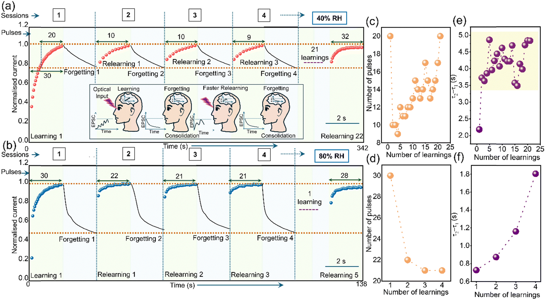Fig. 3 Learning–forgetting–relearning emulated at RH of (a) 40% (Inset: Schematic of the learning–forgetting–relearning process) and (b) 80% with the number of pulses required for consecutive learnings shown on the top and the same plotted in (c) and (d) respectively. The dotted horizontal line (brown) on the top indicates the maximum learning imparted in the session and the bottom one (brown) for the extent of forgetting where the gap in between is used for imparting relearning. The variation of τ₂ − τ₁ (consolidation parameter) with the learning process at (e) 40% and (f) 80% RH for the optical pulses used, t_w = 500 and t_i = 200 ms.

The 21 learning sessions at 40% RH as opposed to 4 at 80% RH reflected during the decay as well. Though decay (forgetting) was allowed for ∼2–3 s at both the RHs, almost 50% decay is observed at 80% RH but only ∼20% at 40% RH (Fig. 3a and b). The slow recombination at low RH results in the contribution of trapped carriers too during relearning (thus, numerous effective learning sessions) which is difficult at high RH due to increased carrier mobility and fast recombination.⁵² The consolidation parameter (τ₂ − τ₁) at 40% RH, increased from ∼2.2 s (consolidation) to ∼3.5 s after the first relearning and gradually raised to ∼5 s during the subsequent relearning (Fig. 3e). The low photocurrents (normalized with respect to a peak response of ∼2.8 nA) account for lesser learning which makes the consolidation possible during the initial learning itself. The subsequent learnings are only incremental to the achieved consolidation. Contrariwise, massive learning at high RH (normalized with respect to ∼65.4 nA) makes it difficult to consolidate information during the first relearning itself (Fig. 3f) and thus shows a gradual increase in the consolidation parameter from ∼0.7 s to 1.8 s with relearning. Eventually, the device experiences fatigue due to continuous optical exposure, and the desorption of the water molecules from the nanofibre surface.^65,66 This decreases the number of charge carriers and thus, the photoresponse resulting in the requirement of a large number of pulses for relearning (see relearning 22 and relearning 5 in Fig. 3a and b, respectively). Similar learning–forgetting–relearning curves are obtained at 40% and 80% RH with first learning occurring with 20 pulses (Fig. S9 and Note S3, ESI†).

The effect of the environment on consolidation is studied by considering a less hydrated environment which declines a person's learning ability faster as opposed to a well-hydrated environment⁵⁰ (see Fig. 4a and b). Considering 40% and 80% RH to be a dehydrated and hydrated environment, respectively, the learning ability is emulated. Initially, 50 optical pulses were exposed on the device at 40% RH (normalized with respect to ∼1.6 nA, Fig. 4c). The photoresponse was allowed to completely decay and return to the base current post-exposure, after which another set of optical pulses was applied. It was observed that the current response decreased as compared to the first exposure. Further, after complete photoresponse decay, a time gap of a minute (these time gaps are deliberately given to study the influence of RH with reading voltage off) was given before the next optical exposure which decreased the photocurrent further. A 10-minute gap decreased the photocurrent considerably and a 30-minute gap brought it to significantly lower values. However, it should be noted that this fatigue behavior exhibited at 40% RH can be recovered by exposing the device to a high RH for a while as shown in Fig. S10 (ESI†). Contrastingly, the same time gaps at 80% RH (normalized with respect to ∼151 nA, Fig. 4d) caused a much lesser decrement than at 40% RH. Fig. 4e shows the quantitative decrement in the photocurrent with time which signifies a ∼80% decrement at 40% RH but a ∼20% decrement at 80% RH. The photoresponse and their variation at other RHs (Fig. S11, ESI†) also indicated ∼80% decrement with lower RHs (40, 50, and 60%) and almost 25% at higher RHs (70, 80, and 90% RH) (Fig. S12a, ESI†).

Fig. 4 (a) Schematic depicting fatigue experienced during learning in the dehydrated and (b) hydrated state. Photocurrent at (c) 40% and (d) 80% RH with a time gap varying from 0 to 30 minutes. Variation of (e) photocurrent, and (f) τ₂ − τ₁ (consolidation parameter) with time at 40 and 80% RH. In all the cases, 50 optical pulses of t_w = 500 ms and t_i = 200 ms are employed.

The consolidation parameter τ₂ − τ₁ as shown in Fig. 4f is ∼40 s which increased to ∼50 s in the consecutive learning at 40% RH. However, the drastic reduction to ∼10 s with the time elapsed indicates poor consolidation similar to that in a less hydrated environment. On the contrary, τ₂ − τ₁ almost remains around 10 s with a slight decrement exhibiting the same amount of consolidation throughout at high RH (Fig. 4f) alike a well-hydrated environment.⁵⁰ Similar consolidation parameters (Fig. S12b, ESI†) were observed at other higher RHs as well. The desorption of water molecules from the surface of the nanofibre with optical exposure^65,66 and the electric field-induced stress in the molecular orientation⁵³ is more pronounced at low RH resulting in faster fatigue. However, at high RH the recovery from induced stress is faster in the absence of an electric field leading to slower fatigue.⁵³ The systematic increase in the optical pulses from 1 to 60 contrary to the constant application of 50 pulses induced fatigue to a lesser extent supporting the above reasoning (a detailed explanation is given in Note S4 and Fig. S13, S14, ESI†).

Though forgetting and consolidation depend on the path of learning and vice versa, learning alone can have different trajectories that might not influence forgetting and consolidation after a certain stage. Fig. 5a shows the schematic of different types of learning with an example of a person being in very noisy surroundings. Initially, the person will be sensitive to the noises (potentiation) but later gets habituated to it. Further, the response to the surrounding cues decreases (depression) and when moved out of that surrounding, it will be eventually forgotten (spontaneous forgetting). The same has been explored at different RHs. Fig. 5b shows the learning at 40% RH by exposing the device to 200 optical pulses (normalized with respect to ∼1.8 nA, t_w and t_i are the same as defined earlier). For the initial 45 pulses, the device shows a significant photocurrent increment depicting facilitation or potentiation. From 45 to ∼75 pulses, photocurrent reaches saturation emulating habituation behavior. After the 75th pulse, up to 200 pulses, the current response decreases showing depression behavior. Post-optical exposure, the photocurrent gradually decreases portraying spontaneous forgetting behavior. A similar learning is observed at 70% RH (normalized with respect to ∼61.4 nA, Fig. 5c) and other RHs too (Fig. S15 and S16a, ESI†). The exposure of the device to optical pulses beyond saturation exhibits depression as well because of fatigue induced by continuous optical exposure. Further, the non-linearity factors for potentiation and depression behaviors at 40% RH (Fig. 5d, the equations used⁶⁷ for fitting are explained in Note S5, ESI†) are ∼4.2 and −0.07, respectively and such variations are known in the literature.^68–70 The consolidation parameter τ₂ − τ₁ values (Fig. 5e and Fig. S16b, ESI†) of spontaneous forgetting are similar to that in Fig. 2c. This indicates that excessive learning will not lead to any significant change in consolidation. Learning without sufficient breaks in between after reaching saturation does not help in effective consolidation as well (Fig. S17 and Note S6, ESI†).

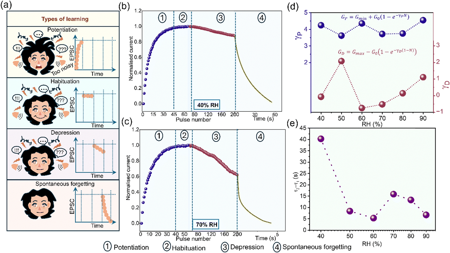Fig. 5 (a) Schematic of the different types of learning. Different types of learning exhibited at (b) 40% and (c) 70% RH. The four types of learning are 1-potentiation, 2-habituation, 3-depression, and 4-spontaneous forgetting. (d) Non-linearity factors for potentiation (γ_P-blue curve) and depression (γ_D-brown curve) at varied RH. (e) The variation of τ₂ − τ₁ (consolidation parameter) with increasing RH.

The photoresponse decay pattern observed in this study has been previously investigated in various active materials, typically described by a double exponential function.^17–19 Here, the initial faster decay is taken to represent the clearing up of excessive information while the latter is due to spontaneous and gradual forgetting. Much of the literature deals with the exponents of the two different decay trends. Hitherto, the transition between the two exponential behaviors had not been given much attention. Through this work, we focused on the transition region and related it to the aspect of working memory consolidation. While working memory consolidation might be influenced by several real-life parameters,⁷¹ in the present setup, the influence of humidity is taken as a token example to examine its effects. Indeed, with humidity as a primary control, we explored the variation of the consolidation parameter in relation to behaviors such as learning–relearning, fatigue, and habituation. Beyond humidity, the consolidation parameter can also be tuned by varying the CS–DMV concentration which influences the nanofiber aspect ratio, thereby affecting both consolidation behavior and decay dynamics. Additionally, the dielectrophoretic alignment of the nanofibres across electrodes further modulates conductivity, directly impacting photoresponse decay and overall learning efficiency.⁷² Future studies may focus on these aspects.

Conclusion

The 1D supramolecular nanofibre device exhibited different EPSC for optical exposure with varying RH with photocurrents 100 times greater at 90% RH as opposed to 40%. Along with EPSC, the PPF index varied from ∼170% to 125% with an increase in RH from 40% to 90%. Indeed, the decay post-optical exposure portrayed the forgetting behavior. However, an important aspect of working memory consolidation is quantified by fitting the decay curves with a double exponential function to completely define the learning and the forgetting process. The defined consolidation parameter τ₂ − τ₁ is insightful in explaining the effective consolidation at low RH and a poorer consolidation at high RH. Given that factors such as rehearsals and environment play an important role in working memory consolidation, learning–forgetting–relearning behaviors were studied which depicted an early consolidation at low RH (40%) and gradual consolidation at high RH (80%). Further, the fatigue experienced and the effect on consolidation have been studied in a dehydrated (40% RH) and a hydrated state (80% RH). Excessive optical pulsing (learning) leads to depression along with potentiation and habituation. A crucial aspect of saturation of consolidation with excessive learning has been demonstrated. The present study defines the complete learning process by introducing the quantification of a crucial aspect of working memory consolidation. The factors affecting consolidation such as rehearsals and the environment have been explored which is discerning and paving the way for the successful emulation of neuromorphic functionalities. Here, humidity serves as an active control modulating consolidation, reinforcing a link between environmental conditions and memory stability. These self-repairing, aqueous-assembled nanofibres enable miniaturization, improved charge transport, and long-term reliability, which might play an important role in integration. Alongside this, the tunable photoresponse decay with humidity and optical inputs makes this system valuable for adaptive learning models, optimizing energy efficiency, and reinforcing learning algorithms and contributes to the advancement of neuromorphic technologies and brain-inspired computing.

Experimental

Synthesis of CS–DMV solution

The detailed synthesis procedure of the CS–DMV solution has been reported previously.⁷³ The synthesis of CS (coronene tetracarboxylate) was achieved through a two-step oxidative benzogenic Diels–Alder reaction between perylene and N-ethylmaleimide, using chloranil and p-hydroxyanisole as reagents, followed by hydrolysis with KOH in methanol. DMV (dodecyl methyl viologen) was synthesized via a selective reaction of dodecyl bromide with one nitrogen of 4,4′-bipyridine to form a monopyridinium ion, which was then reacted with methyl iodide to produce an amphiphilic dicationic bipyridine. To assemble the charge-transfer fibers, a methanol solution of unaggregated DMV was injected into an aqueous solution of free CS molecules (containing 10% v/v methanol). The desired concentration of the CS–DMV nanofibre solution was obtained by diluting it with deionized water.

Device fabrication

The supramolecular nanofibre device was fabricated on a glass substrate which was cleaned by sonicating in distilled water, acetone, and IPA for 15 minutes each, followed by O₃ cleaning. Interdigitated (IDT) electrode patterns were developed by photolithography and Ti was sputter deposited followed by a lift-off process on the glass substrate. On the patterned electrodes, 1 μL of 0.5 mM CS–DMV supramolecular nanofibre dispersion was drop-coated on the IDT microelectrodes and desiccated overnight to remove excess water. The devices for demonstrating device-to-device variability were fabricated by attaching carbon fiber of 6 μm diameter on clean glass substrates serving as a shadow mask after which Ti electrodes were deposited by sputtering. Post deposition, carbon fiber was removed and 1 μL of 0.5 mM CS–DMV solution was dropcoated and desiccated overnight to remove excess water.

Characterization

The device was kept in a cell for varying RH. The RH was varied inside the cell by controlling the flow of N₂ and moisture with the mass flow controllers. The humidity was monitored with a commercial humidity sensor DHT11. The UV light from Thorlabs LED4D067 source was used for optical exposure through the quartz window in the humidity cell. The photoresponse was measured in the Keithley K4200A source-measure unit after taking silver paste contacts from the device. The nanofibre morphology was examined using a scanning electron microscope (Apreo 2 S SEM, ThermoFisher Scientific). UV-visible studies were carried out using a PerkinElmer Lambda-750 UV-visible spectrophotometer.

Author contributions

G. U. K. conceived the idea and supervised the whole work. T. S. R. performed the experiments and measurements. G. U. K. and T. S. R. contributed to the analysis of data, discussions, and writing the manuscript. S. J. G. provided the supramolecule. All authors contributed to the reviewing of the manuscript.

Data availability

The data supporting this article have been included as part of the ESI.†

Conflicts of interest

There are no conflicts to declare.

Acknowledgements

The authors acknowledge the Department of Science and Technology (DST), India, for the funding. The authors thank JNCASR for the facilities. The authors acknowledge the efforts from Dr Suman Kundu in device fabrication. T. S. R acknowledges the INSPIRE fellowship from DST, India. GUK acknowledges support from the J. C. Bose fellowship from SERB, India.

References

1. J. R. Manns and E. A. Buffalo, Fundamental Neuroscience, 2013, pp. 1029–1051.
2. J. Zheng and M. Meister, Neuron, 2024, 113, 1–13.
3. J. T. Wixted, Annu. Rev. Psychol., 2004, 55, 235–269.
4. R. L. Davis and Y. Zhong, Neuron, 2017, 95, 490–503.
5. R. Roesler and J. L. McGaugh, Cold Spring Harbor Perspect. Biol., 2015, 7, a021766.
6. J. M. J. Murre, A. G. Chessa and M. Meeter, Front. Psychol., 2013, 4, 1–20.
7. J. M. J. Murre and J. Dros, PLoS One, 2015, 10, 1–23.
8. C. H. Rankin, T. Abrams, R. J. Barry, S. Bhatnagar, D. F. Clayton, J. Colombo, G. Coppola, M. A. Geyer, D. L. Glanzman, S. Marsland, F. K. McSweeney, D. A. Wilson, C. F. Wu and R. F. Thompson, Neurobiol. Learn. Mem., 2009, 92, 135–138.
9. A. Volianskis, G. L. Collingridge and M. S. Jensen, PeerJ, 2013, 1, 1–13.
10. K. Cotton and T. J. Ricker, Psychon. Bull. Rev., 2022, 29, 1625–1648.
11. S. De Schrijver and P. Barrouillet, Psychon. Bull. Rev., 2017, 24, 1651–1657.
12. T. J. Ricker, M. R. Nieuwenstein, D. M. Bayliss and P. Barrouillet, Ann. N. Y. Acad. Sci., 2018, 1424, 8–18.
13. I. Mondal, R. Attri, T. S. Rao, B. Yadav and G. U. Kulkarni, Appl. Phys. Rev., 2024, 11, 041304.
14. S. Dai, X. Wu, D. Liu, Y. Chu, K. Wang, B. Yang and J. Huang, ACS Appl. Mater. Interfaces, 2018, 10, 21472–21480.
15. T. S. Rao, S. Kundu, B. Bannur, S. J. George and G. U. Kulkarni, Nanoscale, 2023, 15, 7450–7459.
16. S. G. Hu, Y. Liu, T. P. Chen, Z. Liu, Q. Yu, L. J. Deng, Y. Yin and S. Hosaka, Appl. Phys. Lett., 2013, 103, 1–5.
17. D. Sarkar, J. Tao, W. Wang, Q. Lin, M. Yeung, C. Ren and R. Kapadia, ACS Nano, 2018, 12, 1656–1663.
18. S. Lan, J. Zhong, J. Chen, W. He, L. He, R. Yu, G. Chen and H. Chen, J. Mater. Chem. C, 2021, 9, 3412–3420.
19. N. Kumar and A. Srivastava, J. Alloys Compd., 2017, 706, 438–446.
20. C. Yang, J. Qian, S. Jiang, H. Wang, Q. Wang, Q. Wan, P. K. L. Chan, Y. Shi and Y. Li, Adv. Opt. Mater., 2020, 8, 1–8.
21. S. E. Ng, J. Yang, R. A. John and N. Mathews, Adv. Funct. Mater., 2021, 31, 1–12.
22. J. Hur, B. C. Jang, J. Park, D. Il Moon, H. Bae, J. Y. Park, G. H. Kim, S. B. Jeon, M. Seo, S. Kim, S. Y. Choi and Y. K. Choi, Adv. Funct. Mater., 2018, 28, 1–10.
23. R. Jiang, P. Ma, Z. Han and X. Du, Sci. Rep., 2017, 7, 1–8.
24. T. Shi, J. F. Wu, Y. Liu, R. Yang and X. Guo, Adv. Electron. Mater., 2017, 3, 1–10.
25. Z. Wu, J. Lu, T. Shi, X. Zhao, X. Zhang, Y. Yang, F. Wu, Y. Li, Q. Liu and M. Liu, Adv. Mater., 2020, 32, 1–9.
26. X. Yang, Y. Fang, Z. Yu, Z. Wang, T. Zhang, M. Yin, M. Lin, Y. Yang, Y. Cai and R. Huang, Nanoscale, 2016, 8, 18897–18904.
27. B. Zhao, M. Xiao, D. Shen and Y. N. Zhou, Nanotechnology, 2020, 31, 125201.
28. B. Yadav, I. Mondal, M. Kaur, N. S. Vidhyadhiraja and G. U. Kulkarni, Mater. Horiz., 2025, 12, 531–542.
29. R. Attri, I. Mondal, B. Yadav, G. U. Kulkarni and C. N. R. Rao, Mater. Horiz., 2024, 11, 737–746.
30. Y. X. Hou, Y. Li, Z. C. Zhang, J. Q. Li, D. H. Qi, X. D. Chen, J. J. Wang, B. W. Yao, M. X. Yu, T. B. Lu and J. Zhang, ACS Nano, 2021, 15, 1497–1508.
31. M. Pal, M. Kaur, B. Yadav, A. Bisht and G. U. Kulkarni, ACS Appl. Mater. Interfaces, 2025, 17, 5239–5253.
32. S. Mishra, B. Yadav and G. U. Kulkarni, J. Mater. Chem. C, 2024, 12, 18243–18255.
33. J. Liang, X. Yu, J. Qiu, M. Wang, C. Cheng, B. Huang, H. Zhang, R. Chen, W. Pei and H. Chen, ACS Appl. Mater. Interfaces, 2022, 15, 9584–9592.
34. J. Jiang, X. Shan, J. Xu, Y. Sun, T. F. Xiang, A. Li, S. I. Sasaki, H. Tamiaki, Z. Wang and X. F. Wang, Adv. Funct. Mater., 2024, 34, 2409677.
35. B. Sharmila, P. Divyashree and P. Dwivedi, IEEE Trans. Electron Devices, 2023, 70, 1386–1392.
36. F. Wu and T. Y. Tseng, ACS Appl. Electron. Mater., 2024, 6, 5212–5221.
37. T. Zhang, C. Fan, L. Hu, F. Zhuge, X. Pan and Z. Ye, ACS Nano, 2024, 18, 16236–16247.
38. M. Lee, W. Lee, S. Choi, J. W. Jo, J. Kim, S. K. Park and Y. H. Kim, Adv. Mater., 2017, 29, 1–8.
39. S. Seo, S. H. Jo, S. Kim, J. Shim, S. Oh, J. H. Kim, K. Heo, J. W. Choi, C. Choi, S. Oh, D. Kuzum, H. S. P. Wong and J. H. Park, Nat. Commun., 2018, 9, 1–8.
40. H. Tan, Z. Ni, W. Peng, S. Du, X. Liu, S. Zhao, W. Li, Z. Ye, M. Xu, Y. Xu, X. Pi and D. Yang, Nano Energy, 2018, 52, 422–430.
41. S. W. Cho, S. M. Kwon, M. Lee, J. W. Jo, J. S. Heo, Y. H. Kim, H. K. Cho and S. K. Park, Nano Energy, 2019, 66, 104097.
42. D. Li, C. Li, N. Ilyas, X. Jiang, F. Liu, D. Gu, M. Xu, Y. Jiang and W. Li, Adv. Intell. Syst., 2020, 2, 2000107.
43. S. K. Mehta, I. Mondal, B. Yadav and G. U. Kulkarni, Nanoscale, 2024, 16, 18365–18374.
44. J. Wang, B. Yang, S. Dai, P. Guo, Y. Gao, L. Li, Z. Guo, J. Zhang, J. Zhang and J. Huang, Adv. Mater. Technol., 2023, 8, 2300449.
45. T. S. Rao, I. Mondal, B. Bannur and G. U. Kulkarni, Discover Nano, 2023, 18, 124.
46. B. Bannur, B. Yadav and G. U. Kulkarni, ACS Appl. Electron. Mater., 2022, 4, 1552–1557.
47. Q. Li, A. Diaz-Alvarez, D. Tang, R. Higuchi, Y. Shingaya and T. Nakayama, ACS Appl. Mater. Interfaces, 2020, 12, 50573–50580.
48. T. J. Ricker, AIMS Neurosci., 2015, 2, 259–279.
49. J. M. J. Murre, A. G. Chessa and M. Meeter, Front. Psychol., 2013, 4, 1–20.
50. A. C. Grandjean and N. R. Grandjean, J. Am. Coll. Nutr., 2007, 26, 549S–554S.
51. U. Mogera, A. A. Sagade, S. J. George and G. U. Kulkarni, Sci. Rep., 2014, 4, 1–9.
52. S. Kundu, S. J. George and G. U. Kulkarni, ACS Appl. Mater. Interfaces, 2023, 15, 19270–19278.
53. U. Mogera, M. Gedda, S. J. George and G. U. Kulkarni, ACS Appl. Mater. Interfaces, 2017, 9, 32065–32070.
54. G. Gu and M. G. Kane, Appl. Phys. Lett., 2008, 92, 2006–2009.
55. A. A. Sagade, K. V. Rao, U. Mogera, S. J. George, A. Datta and G. U. Kulkarni, Adv. Mater., 2013, 25, 559–564.
56. A. Sumanth, K. Lakshmi Ganapathi, M. S. Ramachandra Rao and T. Dixit, J. Phys. D: Appl. Phys., 2022, 55, 393001.
57. N. Wu, C. Wang, P. M. Slattum, Y. Zhang, X. Yang and L. Zang, ACS Energy Lett., 2016, 1, 906–912.
58. A. Bhattacharyya, M. K. Sanyal, U. Mogera, S. J. Geo and K. Mrinmay, Sci. Rep., 2017, 7, 1–11.
59. S. Kundu, U. Mogera, S. J. George and G. U. Kulkarni, Nano Energy, 2019, 61, 259–266.
60. S. McKenzie and H. Eichenbaum, Neuron, 2011, 71, 224–233.
61. P. Caroni, A. Chowdhury and M. Lahr, Trends Neurosci., 2014, 37, 604–614.
62. C. S. Kim, W. Y. Chun and D. M. Shin, Nutrients, 2020, 12, 1–11.
63. R. Bisaz, A. Travaglia and C. M. Alberini, Psychopathology, 2014, 47, 347–356.
64. S. Mazza, E. Gerbier, M. P. Gustin, Z. Kasikci, O. Koenig, T. C. Toppino and M. Magnin, Psychol. Sci., 2016, 27, 1321–1330.
65. L. Ding, N. Liu, L. Li, X. Wei, X. Zhang, J. Su, J. Rao, C. Yang, W. Li, J. Wang and H. Gu, Adv. Intell. Syst., 2015, 27, 3525–3532.
66. J. X. Qin, X. G. Yang, C. F. Lv, Y. Z. Li, X. X. Chen, Z. F. Zhang, J. H. Zang, X. Yang, K. K. Liu, L. Dong and C. X. Shan, J. Phys. Chem. Lett., 2021, 12, 4079–4084.
67. J. Kang, T. Kim, S. Hu, J. Kim, J. Y. Kwak, J. Park, J. K. Park, I. Kim, S. Lee, S. Kim and Y. Jeong, Nat. Commun., 2022, 13, 4040.
68. D. P. Sahu, K. Park, P. H. Chung, J. Han and T. S. Yoon, Sci. Rep., 2023, 13, 1–16.
69. J. Tang, C. He, J. Tang, K. Yue, Q. Zhang, Y. Liu, Q. Wang, S. Wang, N. Li, C. Shen, Y. Zhao, J. Liu, J. Yuan, Z. Wei, J. Li, K. Watanabe, T. Taniguchi, D. Shang, S. Wang, W. Yang, R. Yang, D. Shi and G. Zhang, Adv. Funct. Mater., 2021, 31, 2011083.
70. J. H. Baek, K. J. Kwak, S. J. Kim, J. Kim, J. Y. Kim, I. H. Im, S. Lee, K. Kang and H. W. Jang, Nano-Micro Lett., 2023, 15, 1–18.
71. R. Roesler and J. L. McGaugh, Cold Spring Harbor Perspect. Biol., 2010, 2, a021766.
72. S. Kundu, S. J. George and G. U. Kulkarni, J. Mater. Chem. A, 2020, 8, 13106–13113.
73. K. V. Rao, K. Jayaramulu, T. K. Maji and S. J. George, Angew. Chem., Int. Ed., 2010, 49, 4218–4222.

---

Footnote

† Electronic supplementary information (ESI) available. See DOI: https://doi.org/10.1039/d5nh00034c

---