Solving an inverse problem with generative models

Abstract

Inverse problems, where we seek the values of inputs to a model that lead to a desired set of outputs, are considered a more challenging problem in science and engineering than forward problems where we compute or measure outputs from known inputs. In this work we demonstrate the use of two generative machine learning methods to solve inverse problems. We compare this approach to two more conventional approaches that use a forward model with nonlinear programming, and the use of a backward model. We illustrate each method on a dataset obtained from a simple remote instrument that has three inputs: the setting of the red, green and blue channels of an RGB LED. We focus on several outputs from a light sensor that measures intensity at 445 nm, 515 nm, 590 nm, and 630 nm. The specific problem we solve is identifying inputs that lead to a specific intensity in three of those channels. We show that generative models can be used to solve this kind of inverse problem, and they have some advantages over the conventional approaches.

---

1 Introduction

In many problems of interest in science and engineering we have some variables we can control (we often call these inputs), and we seek to understand how those variables affect properties we measure (often called outputs). A conventional approach to develop this understanding is to develop a model that relates the inputs to outputs. Typically the model has some fittable parameters, and we might express this model as f(x; p) = y for the inputs x, outputs y and parameters p. The model development typically involves getting data for pairs of (x, y), and fitting a model by linear or nonlinear regression, or through the use of machine learning or other data-driven methods to develop the model. We call this a forward model.

Once we have a model, we can use it to predict outputs for new inputs, for example, given a model to estimate a rate constant as a function of temperature, one might predict the rate constant at a different temperature. The opposite of this, where we ask what inputs give us a desired output, is what we call the inverse problem here. For example, what temperature is required to achieve a specific rate constant? Some models are easy to invert. For example, if our model was: k = k₀ exp(−E_A/RT) as a forward model relating a rate constant to the temperature and some parameters (k₀, E_A), it is straight forward to derive an inverse model: T = −E_A/R/(ln k − ln k₀). Now for a given desired k (assuming we already know the parameters (k₀, E_A)), we can easily compute the input variable T by evaluating the right hand side of that equation with those known parameters and the desired rate constant.

For models that are not analytically invertible, one can resort to nonlinear programming to solve a problem where one iteratively varies x to find the desired y, usually to find a solution to an equation like y – f(x; p) = 0. We presented a complementary approach that uses differentiable programming¹ to derive differential equations that link the input and output spaces through differential equations. Integration of these solutions allows one to map out connected input spaces and output spaces. Thus, with knowledge of one (x₀, y₀) pair, one can integrate along a path from y₀ to a final desired value y_f and obtain the corresponding final input value x_f from the solution.

For well-behaved systems (which we define later), an alternative approach to inverting a forward model is to simply develop a backward model. Here we express the model as g(y; q) = x where again x are the inputs, y are the outputs, and q are parameters associated with the backward model. This model may be data-driven, e.g. using machine learning, or, where possible, may have an analytical form that is used to regress the parameters. Either way, now one simply evaluates g(y; q) at the desired output to identify the input variables that determine it.

Bayesian statistical inversion (BSI) can also be used to solve inverse problems.² This approach is particularly useful when a physical model is available, and prior information is available, or attainable by experimentation. BSI has additional benefits of integrated uncertainty quantification, and incorporation of prior information when available.

In this work, we will explore an approach using generative models for inverse problem solving. The basic idea is that there are ways to use machine learning to make generative models that are capable of generating samples of (x, y) that are consistent with the distribution of those pairs that is known from data. We show that we can effectively solve inverse problems by using conditional generation of samples, where we specify one or more of the values, and then generate the rest of the values. This approach offers some benefits over the methods described above which we discuss.

Conditional generation of samples is not a new idea; we commonly see it today in applications of text generation from large language models, or in image generation. Generative models have been used to solve inverse problems in mechanics.³ Invertible neural networks have been used in inverse problems, e.g. to determine hidden parameters from measurements.⁴ Gaussian mixture models have been used to predict explanatory variables (we call these inputs) from objective variables (we call these outputs).⁵ Generative models have recently been used to generate tabular data.^6,7 This work often seeks to impute missing data. However, when that data contains columns of input and output variables that imputation can be seen in the context of inverse problems; i.e., given some outputs, what are the corresponding inputs? In this work we focus on this use of generative models for solving an inverse problem.

There may be utility in distinguishing between purely data-driven approaches and those that involve a physical model for solving inverse problems here. With data-driven models one typically resorts to generating a learning curve to determine how much data is required to achieve an accuracy goal. In the case of a physical model, one can often use the structure of the model to design optimal experiments that minimize the amount of data required for some level of accuracy, especially when prior information is available. A mix of these approaches is often used. For example, if we have prior knowledge that a system is linear, we may choose a linear kernel in a Gaussian process or the Relu activation function in a neural net, or a linear decision tree model to reflect that. We can incorporate physical information into data-driven models.

We focus on “well-behaved” inverse problems here, by which we mean there is a unique solution to the inverse problem. That is not always true, and we refer to ref. 2 for a thorough discussion of the challenges that can be observed in inverse problems. Here we consider some simple examples for illustration. Consider the relationship y = x². There is no (real value of) x where y = −1. In an inverse problem, it is possible for there to be more than one solution, even when one set of inputs leads to one output. The inverse is not always true; an output might correspond to two or more inputs. In the last example, there are two values of x (x = ±1) where y = 1. The dataset we will use in this work does not have these problems, and in this work we do not consider these interesting issues. Our goal in this work is to introduce and motivate the idea of generative models for inverse problem solutions. We have begun exploring how generative approaches work in these scenarios including nonlinear and many-to-one mapping datasets,⁸ but do not discuss them here.

The paper proceeds as follows. First, we generate an experimental dataset from a model instrument. We use exploratory data analysis to choose some input and output variables. Then we illustrate several approaches to solving an inverse problem of finding inputs that give a corresponding desired output. We start with a forward linear model with nonlinear programming to invert it. Then, we illustrate a partial least squares backward model that is simply evaluated to solve the problem. Finally, we consider two generative approaches: first, generation by directly sampling of a learned distribution; and second, generation by sampling a reference distribution and transforming it to a new distribution.

2 Methods

To illustrate these approaches we will use a simple dataset generated using Claude-Light.^9,10 This simple instrument has an RGB LED with three settable inputs: the red, green and blue channel intensity as a float number from 0 to 1. There is a light sensor with 10 outputs at 8 wavelengths of light from blue to red, a near-IR channel, and a clear channel. The outputs are 16 bit counts that vary from 0 to 2¹⁶-1. The LED and light sensor are connected to a Raspberry Pi which provides the interface to control the instrument via a REST API. The instrument is an adaptation of the SDL-light instrument previously reported,¹¹ and the instrument used in this work is shown in Fig. 1.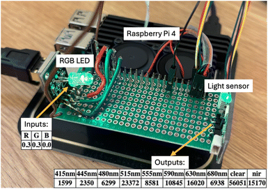

Fig. 1 An image of Claude-light showing the RGB LED that is controlled by the input settings (R, G and B) and typical outputs from the light sensor.

For this study, we generated 100 samples of the three input channels with a Latin hypercube sampling strategy, and measured the outputs for each sample. The sampling strategy is arbitrary, and other choices like uniform sampling or a surface response design of experiments could also be used. The important feature is to span the RGB input space. That dataset is used in each of the examples that follow, and the code used to generate it is available in Section 8.2. We consider four different approaches to solving the inverse problem, which is what inputs are required to achieve an output of 2¹⁴ in three of the output channels. This is an arbitrary choice that was made for convenience (they are all the same) and feasibility (it is possible to get that intensity in each channel).

3 Results and discussion

3.1 Exploratory data analysis

We start by looking at all the data as a pairplot in Fig. 2, which is a convenient way to visualize correlations between variables. In the following sections we will only consider a subset of this data for ease of presentation and discussion. We will focus on the three inputs, and four of the outputs (445 nm, 515 nm, 590 nm, and 630 nm). This shows that many of the outputs are linear in one or more of the inputs, and some do not depend on the inputs much at all. For example the R input channel is highly correlated with the 590 and 630 nm output channels which measure reddish colored light, but it is not correlated at all with 445 nm or 515 nm which are for blue or green lights where there is no overlap of the wavelengths emitted from the red channel and these output channels. The B and G inputs are correlated with the 445 nm and 515 nm respectively, and uncorrelated with the other output channels.

Fig. 2 Pairplot of the data. Bold axis labels are input variables, and italicized axis labels are measured output variables. The main diagonal shows the distribution of values. The off-diagonal plots if there are correlations between the variables. The red channel is highly correlated with two output channels (590 nm and 630 nm), and the blue (445 nm) and green (515 nm) are each correlated with one channel.

For convenience we define several Pandas DataFrames for the inputs and outputs here, as well as a train and test set. These variables are used in all of the subsequent examples.

3.2 Linear forward model + nonlinear program

It is pretty evident from Fig. 2 that the outputs are linear in one or more of the inputs. We can fit a simple linear model: Y = Xp in a least squares sense to estimate the parameters p in the model. We use a library function for the fitting, but one could readily apply the normal equation and basic linear algebra if desired, or a model from .¹² This approach benefits from simplicity in the math and implementation.

In multivariate models it is a challenge to visually show the goodness of fit. We consider a parity plot and R² values for each fit to the train and test data here (Fig. 3). We think it is good practice to combine qualitative visual assessment (e.g. the parity plot) with quantitative metrics like R², MAE, RMSE, etc. Quantitative metrics alone can be misleading, and graphs are useful.¹³

Fig. 3 Parity plots and R² values for the linear regression model for the train and test data sets. Train points are transparent circles, and test points are squares.

There is nothing new in this approach, we simply use it to start a foundation for comparison later. The key observations in the model are that the forward model “looks good” for both the train and test data; parity is good, R² is close to 1. Those are all indicators of a good model. We follow a good practice of evaluating metrics on a test set of data that was not used in the fit.

We now work out our first inverse problem: what RGB settings are required to get an output of 2¹⁴ counts in each of the channels for 445 nm (blue), 515 nm (green), and 630 nm (red)? A traditional way to solve this is with a nonlinear optimizer where we seek the settings that minimize the error between the desired output and predicted output. We use a minimizer here in case there is not an exact solution, and so we find the closest solution. It is noteworthy that the solution here can be sensitive to the objective function, initial guess and optimizer settings.

The model is not difficult to solve here, and there should be only one solution. This is not a general result, there could also either be zero or many solutions in other models. It is only a minor inconvenience (our opinion) that an iterative solver must be used with a guess for the inverse solution. As implemented here, we have no uncertainty quantification; that is possible of course, it just requires more code,¹⁴ or the use of a different model such as Bayesian linear regression or a Gaussian process model.

3.3 Partial least squares backward model

We can avoid the nonlinear solver if we can develop a backward model. In a backward model we want f(outputs) = inputs. Like the forward model, this is also a supervised regression task. We aim to solve the inverse problem again for what input settings (R, G, B) will lead to an output of 2¹⁴ counts in each of the output channels for 445 nm (blue), 515 nm (green), and 630 nm (red). We only have explicit goals for these three outputs, so these can be the only ones in the backward model (there is not an easy way to say the 590 nm output can have any value). Later we will see that generative models allow us to condition on only some of the outputs, but the model we use here does not allow that. If we did know what value we want 590 nm to have, we could add it as an additional output, but it would be easy to pose a problem where there is no good solution. For example, the 590 and 630 nm channels show a lot of collinearity, so it would not be possible to find a setting where 590 nm = 2¹⁰ and 630 nm = 2¹⁴ for example. Instead, they are both likely to have nearly the same value for any R setting.

A simple linear regression might work, but there are known collinearities in the outputs of this data. A partial least squares approach can be used to eliminate the issues with collinearity.¹⁵ In partial least squares we transform the variables into a new orthogonal vector space (thus removing collinearity). We have to choose the dimensionality of that space. Here we choose a three dimensional space because there is not a lot of overlap between the red, blue and green channels, and we expect there to be three independent variables as a result. ¹² provides a convenient library for this approach which we use here. We train on the trainset and evaluate the model quality on the test set (Fig. 4).

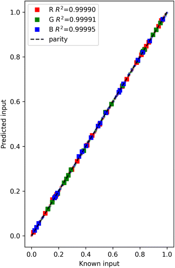Fig. 4 Parity plot for partial least squares backward model. Train data is shown as transparent circles, and test data as squares.

We get nearly the same answer as before. The main advantage of this approach over the previous one is that we do not have to invoke a nonlinear program solver to get the answer we want; we simply evaluate the model for the desired outputs and get the corresponding inputs. We do not need to back solve for what output is expected here; we specified it from the beginning. It is necessary to construct the problem with the specific outputs we want to specify though. Here we had to leave one output channel (590 nm) out because we did not want to specify what value it should have, and in this construction we cannot estimate it. In this approach we also do not have any uncertainty quantification, and it would be considerably more challenging to get it. Of course, other models like Gaussian process models, or Bayesian models that have more integrated uncertainty quantification might be used to mitigate this limitation. Partial least squares is not the only way to build this model. Many other data-driven approaches could be used with various advantages and disadvantages. For example, a machine learning model like a neural network or Gaussian process model might be used, even with a piece-wise linear activation function or linear kernel to leverage our knowledge of the data. Nonlinear models also work with enough data, and care to avoid overfitting.

We note here that it is possible to get unphysical solutions to the inverse problem here. For example, here we ask for the inputs that would yield negative intensities in the output. That is not physically possible, but is mathematically defined with this model. As with other data-driven approaches, we should avoid making predictions outside the known data space.

Alternatively, here we ask for inputs that would lead to intensities greater than can be measured. The instrument cannot do this because the sensor saturates at 2¹⁶-1, and the inputs cannot exceed 1. Nevertheless, the model can extrapolate and provides an answer even though it is not possible in the experiment.

Finally, we note that this example is a well-behaved inverse problem where there is a one-to-one mapping of inputs to outputs. If there was a many to one mapping, this model would not be able to find them all, and may not even fit the data very well. In contrast, with the forward model, one may be able to find multiple inputs from different initial guesses. Thus, these approaches have different benefits for different problems, and it is necessary to know enough about the problem to choose between them.

3.4 Generative samples of a distribution – Gaussian mixture models

We now transition to a generative approach. Here we aim to represent the joint distribution of inputs and outputs with a Gaussian mixture model.¹⁶ Then, we will generate samples from the joint distribution. Each sample will contain the inputs and outputs. Once the distribution is known, we can generate conditional samples, e.g., where we specify the outputs and generate the inputs. See Section 8.3 for an example of conditional generation in two dimensions.

The joint distribution is approximated as a sum of multivariate Gaussian distributions using the Python package.¹⁷ The most important choice to make is how many Gaussians to include in the mixture. The data here is pretty simple: the outputs are each linear in one of the inputs. That suggests we might only need one multivariate Gaussian. The covariance will capture the correlations we observed in Fig. 2. This choice is a classic hyperparameter tuning problem, and one might use any of the existing methods to fine-tune this in a more complex example.¹⁸ In ref. 8 we use a Bayesian Information Criteria (BIC) to identify the number of Gaussians required to minimize the BIC, which finds the best compromise in under/overfitting. Alternatively, there are tools in for this. As with models from , a model is created and fitted with one or two lines of code.

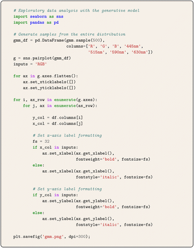
It is not obvious what has been achieved yet, but we have created a model that we can generate samples from. We cannot analyze this in the usual way of parity plots yet because when we generate a sample it contains generated values for the inputs and outputs that are independent of the training data. To see what the model does, we make 500 samples from the fitted model, and then we look at the pair plot of the samples in Fig. 5. The key point to observe is that the correlations look like the same pair plot we saw before in Fig. 2. The distributions on the diagonal look different, but that is just because we used a more uniform distribution (technically a Latin hypercube sampling) before, and the distributions sampled here are Gaussian. That difference is not important here because we only care about the covariances (i.e. the correlations between inputs and outputs) of each distribution.

Fig. 5 Pair plot of samples from the Gaussian mixture model.

On its own it is interesting we can generate samples, but the real value of this model is we can generate conditional samples. That means we can specify some values we want, and then generate the rest. So for an inverse problem, we can specify the values we want for some of the outputs, and then generate the rest of the numbers, which includes the input.⁵

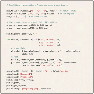
We can use this to make something like a parity plot. We are most accustomed to plot predicted outputs against measured outputs. We can do that here by specifying we want to condition the predictions on the desired inputs. In the implementation, one specifies the columns and values to fix, and then predicts the rest. We use a train/test split as we did before (Fig. 6).

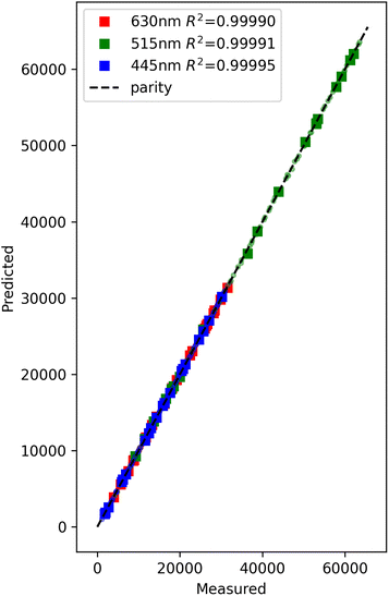Fig. 6 Parity plot of predicted and measured outputs from the GMM model. The train data is shown in transparent circles, and the test data is shown in squares.

To solve the inverse problem, we simply specify the output values and then generate the inputs. In this specific example, the outputs we want to specify are in columns 3, 4 and 6. The code below fixes the values of those columns and then predicts the rest. The inputs we want are in columns 0, 1 and 2 of the predicted values.

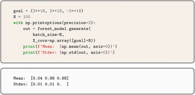
Finally, we can go one step further to estimate how confident we are in the predictions. The function only gives us the most likely value. The method instead draws a number of samples randomly from the conditioned distribution. Then we can consider statistical properties of that distribution, for example, the standard deviation of it to determine how certain we are in its value. If the distribution is narrow, we would be confident in it. In this case, we can say we are confident to three decimal places in the solution.

Generative models can also give unphysical or incorrect answers if conditioned on out of domain values. We again ask for the inputs that would give negative or greater than possible outputs, and see that we again get inputs that are impossible; the inputs must be between 0 and 1 for this instrument. See Section 8.5.1 for an illustration of extrapolation with a GMM model; essentially they extrapolate linearly from the closest Gaussian distribution in the direction of extrapolation.

The Gaussian mixture model is an appealing, intuitive approach to model a distribution as a sum of Gaussian distributions. The big advantage of this is one can condition the resulting approximate distribution analytically, and the predictions should be smooth and continuous. It is likely that this model will start to scale poorly for high-dimensional systems, although we have no direct measure of what “high” means here, but note that the covariance matrices in the model are N × N for N dimensions.

3.5 ForestDiffusion

In the GMM approach we developed a model for the joint distribution of inputs and outputs, and then used conditional sampling to solve the inverse problem by specifying the outputs, and then generating the inputs. Another way to solve this problem is rather than learning that distribution and sampling it, we instead develop a model for the function used to transform one distribution to that distribution (see Section 8.4 for a 1d example). Then we can generate samples by sampling the reference distribution and transforming it to the new one.

There are two methods in this approach with generative models: diffusion models and flow-based models. In a diffusion model noise is added to the data in several steps (in images, this is called a diffusion operation). Then, a model is trained to denoise those samples back to the data. The model can then be used to generate samples of data from the noise distribution. In other words, the model is able to transform noise from a noise distribution into samples with the data distribution. In a flow model, we use a neural network to represent a vector field that determines a “flow” from one distribution (e.g. a Gaussian distribution) to the target distribution that represents the data. A specific model is called continuous normalizing flows (CNF).¹⁹ The idea of this approach is an ODE-driven transformation of a reference distribution, e.g., a Gaussian distribution, to the desired distribution. As an analogy, consider a fluid flowing through a pipe with a parabolic velocity profile. The pipe feeds into a complex geometry that transforms that simple velocity profile to a more complex one. For example, a pipe where the diameter constricts to increase the fluid velocity enough to transition from laminar flow (with a parabolic velocity profile) to turbulent flow (with a more uniform velocity profile) represents a transformation from one distribution to another.

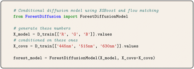
We use the ⁶ implementation which uses a Gradient-Boosted Tree (GBT) and a flow matching technique to learn the vector field that transforms the distributions. This library makes it easy to build a model and we just have to decide in advance which variables we want to condition on, and which ones we want to generate. That is a feature of this implementation, and it is similar to the decision we had to make with PLS. Here, we want to condition on three of the outputs for the counts at 445 nm, 515 nm, and 630 nm in the data, and we want to generate the rest of the numbers in the sample, which includes the inputs and the remaining output channel. The default settings for the work well in this example, and we keep it simple by using them.

As before, we cannot easily assess goodness of fit like we could with parity plots. Instead, we can do conditional generation with this model, we just provide the values to condition on as an additional argument to the method. Here we generate the inputs we expect conditioned on the actual outputs and compare that to the real inputs that led to the measurements. The parity is very good, as are the fit metrics like R² (Fig. 7).

Fig. 7 Parity plot of predicted inputs vs. actual inputs for the output data observed. The train data is shown as small transparent circles, and the test data is shown as solid squares.

We can also generate multiple samples and then do statistical analysis on the distribution of samples as we did with the GMM. This gives an estimate of how certain a prediction is.

It is fair to ask what happens when the model is conditioned on out of distribution data. Here we consider two out of distribution options, the first two outputs are larger than anything considered, and the last one is physically unattainable. The model outputs a result with high confidence. The result is not as unphysical like the GMM case was, but it is also not correct, nor easy to tell that. This model extrapolates like a tree model, and outputs whatever the outermost leaf value is (see Section 8.5.2 for an example). Generative models are not expected to work in extrapolation; these are regions where the underlying distribution is not known. In this example, those regions are not even accessible.

Flow matching and diffusion models are used at very large scales in image generation, and we could anticipate that these models would work well in high-dimension scientific data; albeit with the corresponding need for large datasets.

3.6 Summary

We summarize the four solutions in Table 1. They are practically the same, indicating all four methods are suitable for solving the inverse problem posed here.

Table 1 Summary of the results from each model

Model	Inverse solution
Linear forward	[0.49, 0.24, 0.52]
PLS backward	[0.47, 0.23, 0.52]
GMM	[0.47, 0.23, 0.52]
ForestDiffusion	[0.47, 0.23, 0.51]

---

4 Conclusions

On the surface it appears we solved a simple problem four different ways. That is because we did do that, but the solution was not the main point; the idea of using a generative approach was. Although the dataset here was fairly simple with a linear mapping between the inputs and outputs, it is real experimental data with noise. It is also a prototype for other systems with multiple inputs and outputs, e.g., formulations with multiple components and multiple properties.

We have illustrated four approaches to solving an inverse problem in this work: (1) forward model + nonlinear programming; (2) backward model; (3) conditional sampling of the joint distribution of inputs and output (the GMM); and (4) conditional sample generation by distribution transformation (the model). Each approach has advantages and disadvantages along the dimensions of ease of interpretation, implementation, and uncertainty quantification.

Combining forward models with nonlinear programs is a straight-forward, conventional approach that combines two well-understood and developed concepts. This approach may be subject to limitations associated with the model and the optimizer, e.g., one may only find local solutions, or optimizers may fail to converge. There are decades of experience in this space though, and many options for specialized models and algorithms to mitigate that problem. It is a feature of the forward model approach that an initial guess is required to solve the inverse problem every time, and many must be made to explore the solution space.

Backward models can be equally simple to build as forward models (provided of course the problem is well-behaved, especially with a one-to-one mapping). One still has to choose an appropriate model that captures any nonlinearity, and that there is enough data available to reliably develop that model. The main advantage of this approach is that one simply evaluates the model to solve the inverse problem. A disadvantage is this model does not have forward prediction capabilities, at least without resorting to a nonlinear program solver. A further disadvantage is this approach cannot work if there are many inputs that map to an output.

We showed two generative approaches. These are unique in the sense that they are neither forward nor backward models in principle, but rather either a model of the joint probability distribution linking the input and output data or the transformation function between distributions. At generation time the choice of conditioning variables is what turns the sample into a forward prediction (conditioning on inputs) or a inverse solution (conditioning on the outputs). In the first approach we used a Gaussian mixture model to approximate the joint probability distribution and then used conditional samples of that distribution to solve the problem. In the second approach we used a algorithm to develop a model that transforms one distribution into the target distribution. When these models are good, they allow forward or backward predictions based on conditioning, combining the best features of those individual approaches.

It is pretty remarkable to us that each method relies on roughly the same amount of user code lines (as illustrated in this manuscript). Of course, this is because a tremendous amount of abstraction is hidden away in the libraries that support the code. Nevertheless, this abstraction allows each approach to be used in a just a handful of lines of code.

In this work we only focus on the algorithms for solving the inverse problem, and not on the data selection, or design of experiment, approach. This remains an open challenge. Although many active learning approaches exist for the conventional forward modeling approach, it is less evident how one should sample efficiently for generative models, especially when there is not prior knowledge of how complex the joint distribution will be.

There remains substantial work to do in using generative models for general inverse problems. In this work, we focused on linear models with one-to-one mapping. In principle, one can extend the approach described here to nonlinear models or one-to-many mappings, and those are a focus of current work in our group.⁸ It remains an open challenge to detect extrapolation, out-of-domain predictions and to estimate uncertainty in these models. Finally, there remains work to explore local properties of these models, for example, how smooth are the models, or alternatively how does one avoid overfitting with them? Is it possible to build models with derivative information?

This work shows, in our opinion, that generative methods have significant potential in solving inverse problems, which is exciting. They may enable us to change the difficult job of identifying the type and architecture of a forward or backward model to the challenge of generating data that represents the distribution, training and assessing the generative model. It is likely this approach has broader application than this work shows. One can pose many problems as inverse problems. For example, in parameter estimation we might ask what model parameters are required to yield a given set of observations? Or in an optimization, what inputs yield a minimum defined by some derivatives being zero? In uncertainty quantification, we might ask given some samples from a parameter distribution what distribution of outputs might be expected. Generative approaches may provide new insights and methods to solve these problems.

Data availability

Data for this article and a Jupyter notebook derived from the manuscript and the manuscript source document are available at Figshare at https://doi.org/10.6084/m9.figshare.28726628.

Conflicts of interest

There are no conflicts to declare.

5 Appendices

5.1 Setting up the python environment

We recommend using a virtual environment to reproduce the work in this notebook. is one of the current popular tools for generating virtual environments. This is how we setup the environment for this work. This work was performed on a Mac mini with 64 GB of RAM running macOS Sequoia 15.4.1.

This virtual environment worked for us, but we report the following issues noted during review:

(1) It is possible to have numpy version incompatibilities with catboost and is a library used by .

This looks like an error like this, and it results from a different version of being installed than the one that the library was built with. We did not observe this in the virtual environment used above, but we did observe it trying to run this code in an another virtual environment where the packages were not all installed at the same time.

A solution was reported that was to uninstall both libraries, reinstall numpy, and then reinstall catboost with .

(2) This warning may be seen sometimes. It does not seem to affect anything.

(3) An intermittent multiprocessor shared memory warning was observed by a reviewer. This also does not seem to affect anything.

5.2 Generating the data for this study

We generate and save 100 samples of data. We choose 100 because the experiments are cheap. We use Latin Hypercube sampling which distributes the measurements across the three-dimensional input space with better coverage than simple random sampling.

Each line of rgb.jsonl is a dictionary with the inputs in the “in” key, outputs in the “out” key, and a timestamp for when the data point was taken.

The number of samples, 100, was chosen somewhat arbitrarily. It is probable that fewer samples could be effective if a factorial or Box–Benken type of design of experiments was used.

5.3 2d distribution and conditional sampling

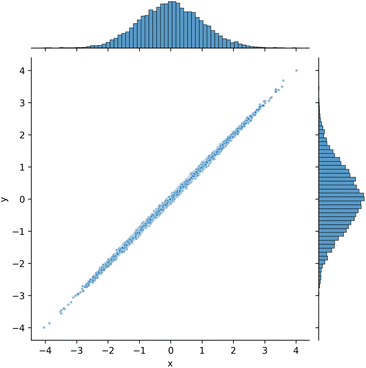
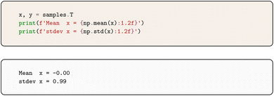
In this section we motivate the idea behind the Gaussian Mixture model approach in this work by examining a single Gaussian distribution in two dimensions. We suppose we have two variables, x, y that are Gaussian distributed and correlated. This is like having a function y = x with correlated noise in both of the variables (Fig. 8).

Fig. 8 A joint plot of two covarying variables.

If we choose one of the variables, say y = 1 then the probable values of x changes. There is an analytical formula to compute this new distribution, but we approximate it here by first finding all the y-values near 1, and then analysing the properties of the corresponding x-values. For comparison, we see as expected the full x distribution is centered near 0 with a standard deviation of 1.

After conditioning though, the distribution consistent with y = 1 is centered at x = 1 with a much smaller standard deviation. There is a formal way to derive the conditioned distribution, but we illustrate it by filtering a thin slice of the data here.

5.4 Transforming a uniform distribution to a Gaussian distribution

It is possible to transform one distribution into another one. One method is inverse transform sampling, which utilizes the inverse of the cumulative distribution function (CDF) to achieve this transformation. For example, there is a known transformation for a uniform distribution x1 to a Gaussian distribution x2:
where erf⁻¹ represents the inverse error function. This function is provided as a special function in scipy. We illustrate how the transform works here (Fig. 9). First a set of uniformly distributed samples is generated, e.g., from a random number generator. Then, the transformation formula is applied to each point. The result is a Gaussian distribution. It is fair to say we have generated a Gaussian distribution this way.

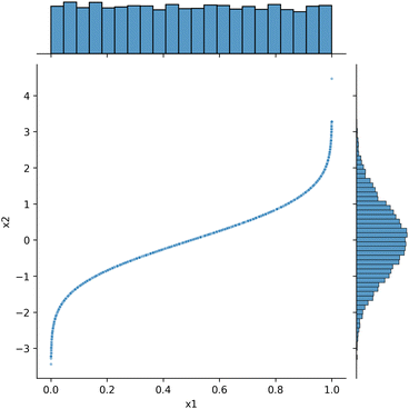Fig. 9 Illustration of transforming a uniform distribution (on the x-axis) to a Gaussian distribution (on the y-axis).

It is possible to use machine learning to learn this transformation function. This idea motivates the idea in this work that it is possible to generate samples of a desired distribution from a reference distribution.

5.5 Extrapolating behaviors of generative models

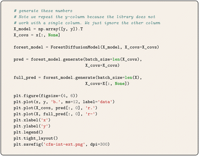
The generative models we present here are still data-driven models, and one should not expect they are reliable outside the training data distribution. We build some intuition in this section. To do that we build a simple dataset that samples a parabola. We create a gap in the middle of missing data. This will enable us to consider what is classically considered “interpolation”, that is predictions that are “inside” the data, and extrapolation, which are predictions “outside” the data. It will become evident in this example that those are not very precise ideas, and that the models are not necessarily accurate in either scenario.

5.5.1 GMM. Based on the previous discussion in the section on conditional sampling of a 2d distribution, we can think of a Gaussian mixture model as a probabalistic piecewise linear model where each Gaussian models a linear piece. As one samples far from the data, a single Gaussian will become dominant, and we could expect then that the model will make linear predictions far from the data. We illustrate that in this example. We choose four components, which should provide two piecewise segments in each chunk of data. The results are shown in Fig. 10, where it is evident that each chuck of data indeed has two Gaussians associated with it. It is also evident that in both interpolation and extrapolation the model behaves as a linear function.

Fig. 10 Illustration of extrapolation and interpolation behavior of a Gaussian mixture model on data sampling a parabola.

5.5.2 ForestDiffusion. It is unclear a priori how a ForestDiffusion should extrapolate, but obvious to us in hindsight. In Fig. 11 it is evident this particular model does not interpolate (predictions “inside” the data) or extrapolate (predictions “outside” the data) reliably. Conceptually a ForestDiffusion model learns a transformation function. That function will only be modified during training by existing data, so in regions where there is no data there is no modification of that transformation function. In this example, this evidently leads to a RandomForest is used in training, and presumably one hits a terminal leaf in the model that leads to constant output away from the data. Other models may behave differently, but it is not expected they extrapolate or interpolate more reliably.

Fig. 11 Extrapolation and interpolation of a ForestDiffusion model for data samples from a parabola.

5.6 About this manuscript

This document was written as a literate program^20,21 using org-mode²² and .²³ This enables the interleaving of narrative text with code and results. The code is executable within the document using a Jupyter kernel, and the results are captured in the document, ensuring the code and data is consistent.²⁴ The document can be exported to LATEX/pdf (for manuscript submission) or a Jupyter notebook (for sharing in a format more commonly used). The org source and derived Jupyter notebook are provided in the supporting information at https://doi.org/10.6084/m9.figshare.28726628.

Acknowledgements

JRK acknowledges AJ Medford for an early suggestion to use generative modeling with Claude-Light to overcome hardware bandwidth for many simultaneous users.

Notes and references

1. V. Alves, J. R. Kitchin and F. V. Lima, An inverse mapping approach for process systems engineering using automatic differentiation and the implicit function theorem, AIChE J., 2023, e18119,  DOI:10.1002/aic.18119.
2. F. G. Waqar, S. Patel and C. M. Simon, A tutorial on the bayesian statistical approach to inverse problems, APL Mach. Learn., 2023, 1(4), 041101,  DOI:10.1063/5.0154773.
3. A. Dasgupta, H. Ramaswamy, J. Murgoitio-Esandi, K. Y. Foo, R. Li, Q. Zhou, B. F. Kennedy and A. A. Oberai, Conditional score-based diffusion models for solving inverse elasticity problems, Comput. Methods Appl. Mech. Eng., 2025, 433, 117425,  DOI:10.1016/j.cma.2024.117425.
4. L. Ardizzone, J. Kruse, S. Wirkert, D. Rahner, E. W. Pellegrini, R. S. Klessen, L. Maier-Hein, C. Rother and U. Köthe. Analyzing inverse problems with invertible neural networks, arXiv, 2018, preprint, arxiv:1808.04730,  DOI:10.48550/ARXIV.1808.04730.
5. H. Kaneko, True gaussian mixture regression and genetic algorithm-based optimization with constraints for direct inverse analysis, Sci. Technol. Adv. Mater.:Methods, 2022, 2(1), 14–22,  DOI:10.1080/27660400.2021.2024101.
6. A. Jolicoeur-Martineau, K. Fatras and T. Kachman. Generating and imputing tabular data via diffusion and flow-based gradient-boosted trees, arXiv, 2023, preprint, arxiv:2309.09968,  DOI:10.48550/ARXIV.2309.09968.
7. D.-K. Kim, D. H. Ryu, Y. Lee and D.-H. Choi, Generative models for tabular data: a review, J. Mechanical Eng. Sci. Technol., 2024, 38(9), 4989–5005,  DOI:10.1007/s12206-024-0835-0.
8. V. Alves and J. Kitchin. Generative machine learning approaches to optimization, chemXiv, 2025, preprint,  DOI:10.26434/chemrxiv-2025-hk886-v2.
9. J. Kitchin. Claude-light: an online, remote instrument for data science education, chemXiv, 2024, preprint, https://claude-light.cheme.cmu.edu.
10. J. R. Kitchin, The evolving role of programming and llms in the development of self-driving laboratories, APL Mach. Learn., 2025, 3(2), 026111,  DOI:10.1063/5.0266757.
11. S. G. Baird and T. D. Sparks, What is a minimal working example for a self-driving laboratory?, Matter, 2022, 5(12), 4170–4178,  DOI:10.1016/j.matt.2022.11.007.
12. F. Pedregosa, G. Varoquaux, A. Gramfort, V. Michel, B. Thirion, O. Grisel, M. Blondel, P. Prettenhofer, R. Weiss, V. Dubourg, J. Vanderplas, A. Passos, D. Cournapeau, M. Brucher, M. Perrot and E. Duchesnay, Scikit-learn: Machine learning in Python, J. Mach. Learn. Res., 2011, 12, 2825–2830.
13. F. J. Anscombe, Graphs in statistical analysis, Am. Stat., 1973, 27(1), 17–21,  DOI:10.1080/00031305.1973.10478966.
14. Ni Zhan and J. R. Kitchin, Uncertainty quantification in machine learning and nonlinear least squares regression models, AIChE J., 2021, 68(6), e17516,  DOI:10.1002/aic.17516.
15. The digital transformation of product formulation, ed. A. Schmidt and K. Wallace, CRC Press, London, England, 2024.
16. J. Giesen, P. Lucas, L. Pfeiffer, L. Schmalwasser and K. Lawonn, The whole and its parts: Visualizing gaussian mixture models, Vis. Inform., 2024, 8(2), 67–79,  DOI:10.1016/j.visinf.2024.04.005.
17. A. Fabisch, Gmr: Gaussian mixture regression, J. Open Source Softw., 2021, 6(62), 3054,  DOI:10.21105/joss.03054.
18. S. Shirinkam, A. Alaeddini and E. Gross, Identifying the number of components in gaussian mixture models using numerical algebraic geometry, J. Algebra Appl., 2019, 19(11), 2050204,  DOI:10.1142/s0219498820502047.
19. Y. Lipman, T. Ricky. Q. Chen, H. Ben-Hamu, M. Nickel and M. Le, Flow matching for generative modeling, arXiv, 2022, preprint, arxiv:2210.02747,  DOI:10.48550/ARXIV.2210.02747.
20. D. E. Knuth, Literate programming, Comput. J., 1984, 27(2), 97–111,  DOI:10.1093/comjnl/27.2.97.
21. E. Schulte, D. Davison, T. Dye and C. Dominik, A multi-language computing environment for literate programming and reproducible research, J. Stat. Software, 2012, 46(3), 1–24.
22. E. Schulte and D. Davison, Active documents with org-mode, Comput. Sci. Eng., 2011, 13(3), 66–73,  DOI:10.1109/MCSE.2011.41.
23. scimax, https://github.com/jkitchin/scimax is an Emacs starter kit that customizes it for scientific publishing.
24. J. R. Kitchin, Examples of effective data sharing in scientific publishing, ACS Catal., 2015, 5(6), 3894–3899,  DOI:10.1021/acscatal.5b00538.

---