Large language models for knowledge graph extraction from tables in materials science

Abstract

Research in materials science increasingly harnesses machine learning (ML) models. These models are trained with experimental or theoretical data, the quality of their output hinges on the data's quantity and quality. Improving data quality and accessibility necessitates advanced data management solutions. Today, data are often stored in non-standardized table formats that lack interoperability, accessibility and reusability. To address this issue, we present a semi-automated data ingestion pipeline that transforms R&D tables into knowledge graphs. Utilizing large language models and rule-based feedback loops, our pipeline transforms tabular data into graph structures. The proposed process consists of entity recognition and relationship extraction. It facilitates better data interoperability and accessibility, by streamlining data integration from various sources. The pipeline is integrated into a platform harboring a graph database as well as semantic search capabilities.

---

1 Introduction

Materials science is increasingly implementing data-driven approaches, marking the much-quoted shift towards the fourth paradigm.^1,2 The use of emerging artificial intelligence (AI) tools in materials research promises to accelerate materials discovery by guiding efficient and time-saving exploration through high-dimensional materials parameter spaces.^3–7 In the growing field of autonomous experimentation, machine learning models are deployed to plan experiments^8–11 while computer vision tools automate imaging analysis.^12–15

The quality and availability of data are crucial in this realm. Data generation in materials science is frequently tied to short-term projects and is considered time-consuming and costly, leading to the creation of many small and scattered datasets.^16,17 Data management in research labs typically relies on relational databases or file systems, predominantly filled with tables. Those tables are rich data assets; however, information on how data points across different columns are interconnected is often only implicitly provided. The lack of data management standards, therefore, leaves valuable data silos scattered with very limited accessibility and interoperability among labs or institutions.^18–20

Several recent papers have emphasized the need for openly accessible databases; however, data heterogeneity due to varying length scales and structural complexity of materials presents intricate technical challenges.^21,22 Consequently, databases are often limited to single length scales, highly domain-specific, and focused on chemical elements and compound properties that do not depend on microstructure.^23–30 Thus, the materials science community is experiencing a trend toward information silos separated by domain, design, or exploration space, hindering the full potential of AI methods.³¹ This separation complicates finding answers to generic research questions. Filtering a corpus of materials for desired properties or identifying processing conditions associated with desired materials properties often requires consulting domain experts or scientific literature.³²

Knowledge graphs are promising data structures, responding to these challenges. They consist of nodes and relationships forming a network of connected entities.³³ These relationships make information and contextualized data machine-readable, facilitating the integration of tools to analyze, organize, and share information. Furthermore, graphs excel in representing highly heterogeneous data due to their focus on connectivity, which provides a high degree of flexibility.^34,35 Materials science increasingly uses knowledge graphs to integrate and organize data from literature, databases, and ontologies.^35–37 To elevate them to viable data management solutions on lab-scale and beyond, these tools need to be broadly appealing to materials science.

Attractive data management solutions provide intuitive mechanisms for data storage and retrieval, streamlining the process for data owners by removing unnecessary complexity. Moreover, they ought to reduce their usage barrier, ensuring smooth integration into the user's routine data practices, with minimal interruption.¹⁷ The capacity to mine existing data, derive insights, and integrate them into one's data assets is a crucial feature of data management systems. Thus, broad adoption of graph-based data management solutions requires tools that facilitate the migration from existing tabular data assets to knowledge graphs. Knowledge extraction is an emerging field aiming to extract information from structured and unstructured sources³⁸ and is increasingly applied in the materials science domain.^39,40 Recent advances in natural language processing through the availability of Large Language Models (LLMs) provide novel disruptive tools in this field.^41,42 LLMs excel in inferring context and meaning of unseen data without the need for expensive training. This eases the implementation of LLM-enabled knowledge extraction tools, making them attractive for data management solutions.

In a recent publication, we proposed a data model for graph databases⁴³ that follows the logic of the Elementary Multiperspective Material Ontology (EMMO).⁴⁴ An ontology is a structured framework that defines and categorizes the concepts, entities and their relationships within a specific domain. The proposed data model is able to represent experimental workflows in materials science with any desired degree of granularity. Entities within the database are labeled via a semantically connected system of nodes that span a wide range of processes, matter and quantities (see Fig. 1). These labels are based on the EMMO and BattINFO, a domain-specifc EMMO extension focused on batteries and their characterization.⁴⁵ The database aims to help research groups manage their data assets in an intuitive way while making it interoperable with other data vendors.

Fig. 1 Schema of the proposed graph data model (a) and example of the labeling system (b).

In this study, we introduce a knowledge graph extraction pipeline to improve the efficiency of populating graph databases with existing table data. The pipeline semi-automatically transforms tables into connected knowledge graphs that follow the data model we proposed in Fig. 1. The extraction process utilizes LLMs to infer meaning from headers and extract information from tables. We divided the process into four stages, which can be verified by the user through a graphical user interface, ensuring the high quality of the knowledge graph. To enhance the cost efficiency and scalability, we integrated various caching strategies to streamline the extraction process from known tables.

Comparatively, alternative solutions—such as Microsoft's GraphRag⁴⁶ and manual data transformation approaches—often require expertise in database querying languages or extensive iterative prompt engineering. While these methods are viable, they tend to be labor-intensive and face scalability challenges due to their technical complexity. In contrast, enterprise cloud data management platforms like Databricks,⁴⁷ Google Cloud,⁴⁸ and Splunk⁴⁹ are designed to integrate seamlessly with standard workflows, providing streamlined and robust data operations. However, their architectures are generally optimized for more homogeneous data, which makes it difficult for them to natively handle the high complexity and heterogeneity inherent in scientific data. Consequently, effective data management in the scientific domain should seamlessly integrate into existing data handling routines. Thus, data management should not impose significant technical overhead or require specific expertise from researchers, while allowing them to accommodate the full complexity and interconnected nature of their data.

In the following, we thoroughly discuss the methodologies and metrics of the extraction procedure and its results. This article is relevant to those interested in using our data management system or engaging in knowledge extraction in different scientific domains.

2 Methods

The generation of a knowledge graph involves two key processes, node extraction and relationship extraction. Node extraction from tables is a multi-step procedure. Initially, each column is assigned a node type (e.g., matter, property). Next, the attribute type of each column is identified (e.g., Name, Value). Finally, columns representing different attributes of the same node are aggregated.

The entities extracted through this process are then used to infer relationships, constituting the build-up of a knowledge graph. The following sections provide an overview of the data types encountered in this study, introducing the input and output and delineating the specifics of the extraction pipeline.

2.1 The input: tables

The pipeline is designed to transform tables, which are the most common format for researchers to store, analyze, and communicate their data. It accepts CSV files as input and requires the tables to be flat—that is, each row represents a data record and each column contains specific values (e.g., numbers, strings, or dates). In contrast, nested tables allow columns to contain sub-tables or arrays. We tested and validated our pipeline on a dataset of 15 flat tables. We minimized bias in our test dataset by ensuring high heterogeneity; the dataset comprises data from various subdomains of materials science, with data from measurements, syntheses, simulations, properties, organizational data, and single processing steps. We also varied the data sources by incorporating tables from self-driving labs and from different research groups. Table 1 shows an excerpt of one such table that can be transformed into a graph. The pipeline was tested on tables with between 4 and 90 columns. Since only the table headers paired with sample rows are used in the transformation, the total number of rows does not affect the process. The tables are available in our GitHub repository.⁵⁰

Table 1 Excerpt of a table from the dataset we used to test and evaluate our pipeline. The whole dataset can be a accessed in our GitHub repository

Drymilltime (h)	Drying T (°C)	Catalyst	Ionomer	Equiv. weight	I/C
6	55	F50E-HT	Aquivion	790	0.7
24	55	F50E-HT	Aquivion	790	0.7
48	55	F50E-HT	Aquivion	790	0.7
6	55	F50E-HT	Aquivion	790	0.9
24	55	F50E-HT	Aquivion	790	0.9
48	55	F50E-HT	Aquivion	790	0.9
6	55	F50E-HT	Aquivion	790	1.1
24	55	F50E-HT	Aquivion	790	1.1
48	55	F50E-HT	Aquivion	790	1.1
⋮	⋮	⋮	⋮	⋮	⋮

---

In materials science, these tables typically describe entities such as materials, components, devices, chemicals, properties, measurements, manufacturing steps, and processing conditions. The goal is to extract these entities and contextualize them by inferring relationships among them.

For example, the excerpt in Table 1 contains a column titled “Ionomer” immediately followed by a column labeled “Equivalent Weight” that holds numerical values. To retrieve meaningful information, the pipeline must extract a matter node representing the ionomer cell “Aquivion” and connect it to a property node labeled “Equivalent Weight”, which carries the numerical value of 790 and the unit g mol⁻¹. Given the significant variations in table structures and header terminologies, our pipeline is designed to be agnostic to both structure and terminology, enabling it to process a wide range of tables without prior knowledge of their layout. The pipeline leverages LLMs to extract data within the domain of materials science, with a particular focus on energy materials.

2.2 The output: knowledge graphs

The graph model we introduced in a previous publication follows the logic of the Elementary Multiperspective Material Ontology (EMMO). The graph model consists of the node types and relationships shown in Fig. 1.⁴³ These nodes and their relationships are capable of representing materials and processes in materials science. To capture domain-specific terminologies and ensure data interoperability, we introduced a labeling system for our graph database. This labeling system comprises classes such as matter, property, parameter, measurement, simulation, and manufacturing, along with their subclasses. These tree-like structures were derived from EMMO and its domain-specific extensions like BattInfo. Each ingested data point is labeled by linking it to a label node via an IS_INSTANCE relation (see Fig. 1(b)). Label nodes are semantically connected via IS_A relations to indicate parent/child relationships. The label nodes form taxonomies of the matter, manufacturing, property, and property nodes. This structure semantically embeds alternative labels in a tree format, as each node is connected to a specific label node and indirectly linked to all its sub- and parent classes. The labeling of each node via a semantically contextualized label is the foundation for a semantic search functionality that allows for highly specific and very broad querying of the knowledge graph. Additionally, we introduce a tool for the dynamic extension of the labeling system (see Section 2.4). The labeling system is available on our GitHub repository as .owl files.⁵¹

2.3 The pipeline

Transforming table data into a knowledge graph requires extracting implicit information, which involves domain knowledge and understanding of table structures. Due to the variety of table structures, rule-based algorithms are insufficient. We utilize LLMs for their domain knowledge and ability to interpret table content and structures. To address scalability, we implemented caches (look-up tables) for tables and columns to reduce LLM usage for known data. The latter allows known table structures to be processed without the use of LLMs. Feedback loops and validation functions enhance accuracy and determinism. Our pipeline processes only the table headers and a sample row with altered numerical data to ensure data security while using the APIs of OpenAI. The transformation task is divided into four sequential steps, each adding context and information. Fig. 2 provides a schema of the full pipeline.

Fig. 2 Schematic overview of the extraction pipeline on the example of a specific table. The pipeline consists of a node type extraction (see Section 2.3.1), node attribute extraction (see Section 2.3.2), node extraction (see Section 2.3.3), and relationship extraction (see Section 2.3.4).

2.3.1 Node type extraction task. Each table column is assigned to a specific node type (e.g., matter, property, property) by converting the header and a sample cell into embeddings. Embeddings are high-dimensional vector representations of human language. These embeddings are compared to a static pool of various examples for the different node types. Non-classifiable or ambiguous headers are flagged for user assignment.

We use the OpenAI embedding generator as it has shown high accuracy in benchmarking, especially in classification tasks. To improve the accuracy of this step, the table header of each validated classification is transformed into an embedding and added to the pool of node examples. The candidate selection uses cosine similarities to find the most similar vector in the pool of examples.

The process is encapsulated into a classifier Python class that iterates over all table headers, creates embeddings from the table header and the sample cell, identifies the best match from the pool of examples, and returns a dictionary with each header representing a key with its node type as the value. As the node type assignment of each header is an isolated task, it can be easily parallelized.

Fig. 2 presents an example for the node type extraction. The assignments of the correct node types to the columns that contain matter nodes are straightforward as they contain headers that are semantically very close to matter and can therefore be easily assigned to an example for the node type matter. A challenge can arise with the heading “Method” as it has a high semantic overlap with measurement and manufacturing and could therefore be attributed to both node types. Since manufacturing steps and measurements have different methods (e.g., “mixing”, “imaging”, etc.) both node types show a high semantic overlap with the word “Method” alone. For that reason, the header and sample cell are transformed into an embedding. The word “mixing” is less ambiguous and, therefore, the embedding from the header and the sample cell can successfully be assigned to the node type manufacturing.

2.3.2 Attribute extraction task. After assigning node types, the next step identifies node attributes in each column. The AttributeClassifier generates embeddings for headers and sample cells by comparing them to a pool of candidates. The best match is identified following the same logic as the node type extraction.

In Fig. 2, we illustrate the attribute extraction process. In the example, columns containing Identifier attributes contain “ID” in their headers, while those listing material names reference well-established materials in the cells and headers. Columns with property and parameter values display numerical entries that can be directly associated with the corresponding attribute, value. Because the node type of each column is determined in the first step, the range of possible attributes is constrained. For example, matter, manufacturing, and measurement nodes include an identifier attribute, whereas parameter and property nodes do not. Thus, knowledge of the node types, along with the unambiguous headers and cell contents, makes the assignment of each column to the correct attribute straightforward.

2.3.3 Node aggregation task. The third step aggregates columns into nodes, combining attributes of the same entities to form cohesive nodes. We leverage LLMs to overcome limitations of rule-based approaches. We implemented a NodeAggregator, NodeEvaluator, and NodeCorrector class for each node type, which use Chat-GPT-4-o. The node extraction is executed in parallel for each node type, with results validated and corrected iteratively.
2.3.3.1 NodeAggregator. Each NodeAggregator of a specific node type consists of a prompt generator and an LLM agent. The NodeAggregator transforms the given table data into a list of nodes that follow a node-type-specific JSON schema (see Fig. 3). The prompt generator of a specific NodeAggregator accepts all table columns that contain attributes of its node type, along with the context provided by the user and all table headers as additional context. From this input data, it generates a prompt that requests transforming the given table headers into a list of nodes while considering the context and the table structure. The generated prompt is used to initialize an LLM agent with a node-type-specific setup message.

Fig. 3 Schematic representation of an Extractor, Validator, and Corrector class.

The agent is given the following information:

(1) Introduction and general task (system message).

(2) Explanation of the expected output (schema).

(3) Context provided by the user (user input).

(4) Examples (few-shot).

Each agent is initiated with a fixed system message explaining the task and providing general input and guidelines. Additionally, we employ few-shot learning by generating an artificial conversation history in which the agent was given a table and produced the correct nodes. These examples serve as valuable guidelines on how to aggregate nodes correctly and which format to follow. The actual prompt is automatically generated and contains the table headers, a sample row, and a string of additional context provided by the user. Fig. 3 represents the general structure of an LLM-enabled pipeline containing extractor, validator, and corrector classes. Node aggregation and relationship extraction are implemented following this general structure and vary only in inputs and static components.

2.3.3.2 NodeValidator. The NodeAggregator's output is forwarded to a corresponding NodeValidator instance, which analyzes the output for logical mistakes. The specific validation functions depend on the node type and can be checked in the GitHub project. In general, the validation consists of logic checks implemented in a rule-based approach that aim to improve the determinism of the NodeAggregator output. They check for typical mistakes the LLM agent makes, such as assigning the same column to attributes of different nodes. Additionally, the NodeValidator checks for any violation of the graph data model. For example, a property or quantity node always needs the attribute name, value, and unit to be non-null. Each validation function returns the wrongly aggregated nodes or True, if the agent did aggregate correctly, considering the specific aspect that the validation function inspects. After all validation functions are executed, the NodeValidator creates a dictionary containing each validation function and its output.
2.3.3.3 NodeCorrector. These validation results are used by the NodeCorrector class to refine the NodeAggregator results. Each validation function is mapped to one correction function that generates a prompt, asking for revision by providing the incorrectly aggregated nodes along with an explanation of the error, as well as optional error-specific context. Each mistake detected by the NodeEvaluator is transformed into a revision prompt resulting in a list of revision prompts. This list of revision prompts is merged into a single prompt to the LLM that lists all mistakes and asks for revision. This prompt is given to an agent initiated with an identical conversational memory as the agent of the initial aggregation. The NodeCorrector generates a revised list of nodes that can be validated and corrected again in an iterative refining process.

To clarify the node aggregation procedure, we will follow the aggregation of all matter nodes in the example of Fig. 2. The agent of the MatterNodeAggregator receives a prompt containing the table, user context, and instructions to transform columns 1, 2, 3, and 6 into nodes. The agent should then correctly assume that the table provides information about the fabrication of a catalyst ink, and therefore propose the creation of three matter nodes per row: one for the ionomer, one for the catalyst, and one for the catalyst ink. The catalyst name and identifier must be extracted from columns 1 and 2. The matter node representing the ionomer has a name that is taken from column 3. The node representing the catalyst ink has an identifier in column 6. Since no column provides a name for the catalyst ink and it is a crucial attribute, the agent needs to infer it (for example, “catalyst ink”) from the header of column 6. Each row of the table can thus be transformed into three matter nodes, with attributes varying by row, except for the name of the catalyst ink node, which is inferred from the table headers. If the MatterNodeAggregator does not infer the name “catalyst ink” for the matter node representing the catalyst ink, the MatterNodeValidator would detect this during its sanity check. In that case, the MatterNodeCorrector would be invoked to correct the error by inferring the missing name attribute.

2.3.4 Relationship extraction task. The current state of the table transformation represents the table as a list of nodes, with all columns aggregated into nodes of various types. However, to form a complete graph, relationships must be inferred from the table's content. Since most tables contain these relationships only implicitly, extracting them requires an understanding of the information hidden within the data. The implementation of relationship extraction follows the same structure as node extraction (see Fig. 3).
2.3.4.1 RelationshipExtractor. For each relationship type, a specific RelationshipExtractor was implemented that extracts an initial list of relationships from the table. Each instance consists of an LLM agent and a prompt generator. An instance of a specific RelationshipExtractor is initialized with two lists of nodes, the context provided by the user, the table headers, and a sample row. The prompt generator generates a query that requests reasonable relationships to connect pairs of nodes. As each relationship type is extracted separately, only nodes with the correct types are given as possible candidates. The “HAS_PROPERTY” relationship connects a matter node with property nodes, which means that the HasPropertyExtractor receives a list of matter nodes and a list of property nodes as the main input. Since a knowledge of the complete table structure is crucial for a successful relationship extraction, the prompt also contains the table's header and first row as well as the context given by the user. The LLM-agent of each extractor instance is initiated with a relationship type-specific setup message containing an explanation of the task, the input data, relationship-specific rules and tips, as well as examples with a chain of thought to further improve accuracy.
2.3.4.2 RelationshipValidator. For each relationship type, one RelationshipValidator class was implemented. Depending on the relationship type, these classes execute a number of validation functions to check the output for logical errors. These validation functions check graph logic, such as the connectivity of the graph or its nodes, or the cardinality of certain relationships. Each validator generates a dictionary containing the executed validation functions and their results. The classes' structure is therefore very similar to the NodeValidator, as both run validation functions and return the results as a dictionary.
2.3.4.3 RelationshipCorrector. Each evaluation function has a corresponding correction function that generates a prompt specifying the identified mistakes and requesting a revision. The RelationshipCorrector uses the output of the validator and generates a list of prompts that are concatenated into a single prompt that lists all extraction errors. The corrector then initializes a new agent with the same conversational memory as the RelationshipExtractor and requests a revision of the results, stating all detected errors. The output is a refined list of relationships that can be evaluated and corrected again.

The relationship extraction in Fig. 2 can be illustrated using the example of the HasPropertyRelationshipExtractor. This class extracts the HAS_PROPERTY relationships that connect matter and property nodes. In this example, the extractor would receive a list of all matter nodes (e.g., the ionomer, the catalyst, and the catalyst ink) as well as a single property node (e.g., the I/C ratio). The agent must then decide to which matter node the property node belongs. This can be inferred either by recognizing that “I/C” stands for “ionomer to catalyst ratio”—indicating it is a property of the catalyst ink, or by analyzing the table structure, since the property node's column is directly adjacent to the catalyst ink node's column.

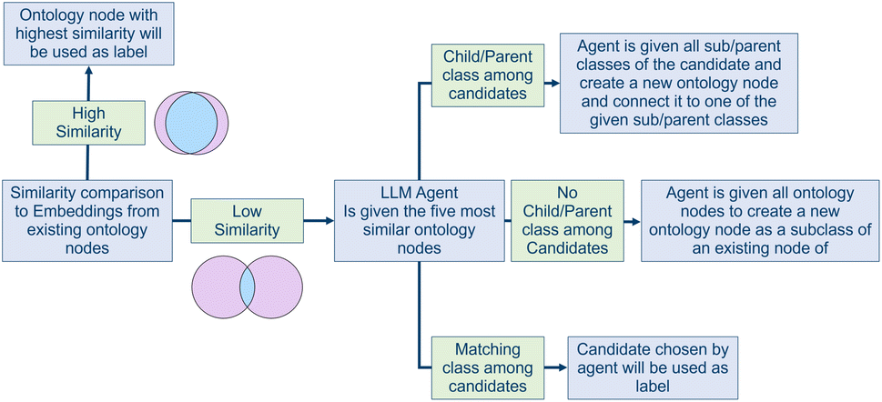
2.4 Label assignment

To make the data searchable and interoperable, the extracted nodes need to be labeled correctly. Labeling data means that each Name attribute within the extracted nodes is processed and mapped to a label node within the graph database's labeling system. If no adequate label can be found within the database, an LLM agent is used to create a new label node and extend the existing labeling system. This step is essential to enable effective querying of the database later on. It requires different instances of the same kind to be assigned the same label, so that they can be searched and found with the same queries. To enhance interoperability, the used labels should follow lingo and terminology that at least parts of the community already agreed on.

2.4.1 Generation of the labeling system. As a basic labeling system, we ingested the matter, Quantity, and Process branches of EMMO and its BattInfo extension into the graph database. These branches form a taxonomy of label nodes that can be used to classify the extracted data. A branch here is a tree structure that contains each top-level label node and its subordinate nodes. For each label node within the branches, we generated a list of alternative labels as well as a short description. As the three branches contain more than 1000 label nodes, adding alternative labels and descriptions to each node is done automatically using the Chat-GPT-4-turbo module of OpenAI. The label node's name, its alternative labels, and the description are then used to generate embeddings that capture the full semantic bandwidth of each label node. The embeddings are generated by the OpenAI API and stored in the graph database as vector nodes connected to the label nodes.

2.4.2 Similarity-based classification. Finding the appropriate label for an extracted node is a classification task and requires finding the most similar label node within the taxonomy (e.g., the labeling system). Identifying the correct label is done using embeddings and Chat-GPT-4-turbo. The name of the node that needs to be labeled is transformed into an embedding. The embedding is then compared to the embeddings stored within the labeling system of the database, and the best matching label node is identified by calculating and comparing cosine similarities. If the highest similarity score does not exceed a threshold value of 0.95, it is very likely that no label node sufficiently represents the given name.

2.4.3 LLM-assisted extension of the taxonomy. In that case, we employ an LLM agent with the task of finding a matching label node or extending the taxonomy dynamically. The agent is initiated with a node-type-specific setup message containing the task, relevant hints, rules, and examples. Furthermore, the agent receives the node name that needs to be labeled, as well as the most similar label nodes as possible candidates. The agent's task is to identify a label node from among the candidates that either adequately describes the node or could describe one of its “child” or “parent” label nodes. This prompt can lead to three different outcomes:

(1) No match found: if none of the candidates is a suitable label node, or a child or parent class of the unlabeled node, the agent is given all possible labels of the given node type. If the unlabeled node is a matter node, this means all label nodes that are children of the label node named “matter” are forwarded to the agent. Among them, the agent chooses a label node that represents a parent label of the unlabeled node. Then, the agent is asked to suggest a new label and additional child labels—if necessary—to seamlessly extend that branch. The output of the agent is used to create new label nodes within the graph database. They are used to label the unlabeled node and extend the existing taxonomy.

(2) Adequate match found: if one of the candidates represents an adequate label for the node, the task ends and the node gets assigned the label chosen by the agent.

(3) Subclass/parentclass found: if one of the candidates is a parent or child label of the unlabeled node, the agent is given all parent or child labels of that candidate. The agent then has to identify the semantically closest label node and generate a new label node that adequately represents the extracted node. To improve the quality of the extension, the agent can suggest additional labels to smooth the branching. The output of the agent is used to create new label nodes, connecting them to the existing taxonomy. The unlabeled node is then stored within the graph database and linked to the newly generated label node.

The complete procedure is depicted in Fig. 4. As the correct extension of the labeling system is crucial to make the data retrievable and interoperable, all newly added label nodes are flagged for curation by the database admins.

Fig. 4 Schematic overview of the labeling workflow.

2.5 Caching

Currently, using the pipeline is slow and expensive for unseen tables. To compensate for that drawback, we implemented look-up tables to allow wide adoption of the pipeline. These look-up tables are a means to cache graphs for recurring tables or table parts. If a known table needs to be transformed, the cache can be used to bypass the LLM usage, which is the time- and cost-determining part of the graph extraction. Tables and their parts are only added to the cache and look-up tables if their transformation has been validated by the user and the admin.

Two ways of caching have been implemented:

Single-column cache: single-column caches contain the headers of individual columns and the assigned node types and attributes. Columns that contain already known table headers can be cached, and the first two steps of the transformation pipeline can be skipped. Additionally, table headers with already correctly extracted labels and attributes are transformed into embeddings and added to the pool of examples for the labels and attributes they represent. These additional embeddings facilitate type and attribute extraction of headers with similar wording and therefore help boost the accuracy of the first two steps of the pipeline.

Table cache: as researchers or self-driving labs often generate the same table structures, caching full graph extraction is crucial to enhance the scalability of the pipeline. We implemented look-up tables that store the table headers and the resulting graph of each validated extraction. If already cached tables need to be transformed into graphs for ingestion into the database, the cache is activated and the correct graph can be directly requested from the look-up table.

All look-up tables are within an SQL database and accessible via the django-admin user interface. Each transformation procedure generates one single-column cache for each table column and one table cache entry for the full table. These new cache entries are directly validated by the user through the GUI. Through the django-admin interface the cached tables can be checked and validated by the admin. After validation by the database administrator, the columns and tables are fully cached.

3 Results

The pipeline operates in a semi-automated fashion, requiring the user to verify the results of each step when the table to be ingested is unknown. Successful extractions are cached, allowing fully automated graph extraction for known table structures. The semi-automated approach ensures high-quality graph extraction, as the transformation from a table to graph can result in multiple possible graphs if the table headings and structure are ambiguous. This uncertainty accommodates the diverse and unrestricted nature of table structures and terminology that we allow as users' inputs.

To set up a robust pipeline, it is necessary to optimize each step. The first two steps are classification tasks, to assign a node type and node attribute to each column. Optimizing node type and attribute extraction (see Sections 2.3.1 and 2.3.2) requires optimization of:

• Examples: each column is assigned to a node type and node attribute by a similarity comparison to a pool of examples (e.g., examples for the node type Parameter might be: “Operating Condition”, “Process Parameter”, “Heating Speed”).

• Input: depending on the format and structure of the examples, the input for the classification can be optimized (e.g., Heading:Sample_Cell, Heading, “Key”: Heading, Value: “Sample Row” are different ways to generate input for a similarity comparison and will lead to different results).

• Matching: the logic of how the correct node type/attribute is chosen can be varied (e.g., a naive approach is to select the example with the highest similarity).

The subsequent steps, which extract nodes and relationships, mainly depend on prompt engineering. The accuracy here was improved by prompt engineering and iterative tweaking of the input to the LLM agent. Prompt engineering is very expensive; therefore, we optimized the prompts on tables with high complexity that contain nodes and relationships of all types and most labels. Increasing accuracy requires optimization of the following:

• System message: the system message contains the general information and task the LLM Agent is given (e.g., “You are a world-class node extracting algorithm…”).

• Prompt: the actual prompt the agent is given to extract nodes/relationships from a given input.

• Examples: examples that are given to the agent that show how to correctly extract data from a given input.

• Schema: the desired output format that contains small descriptions of the parts of the output.

• Input data: the input data is part of the prompt. It is important to include it in a way that is easy to process and contains exactly the information and context that is needed to solve the given task.

The final parameters for every step are made available on our GitHub repository.⁵²

3.1 Evaluation

3.1.1 Evaluation of the classification tasks. The node type and node attribute extraction are evaluated using precision, recall, and the F₁ score as metrics:

We evaluated the classification tasks on the headings of all tables listed in the data repository. Additionally, we created an artificially generated dataset of 100 heading/sample_cell pairs for each node/attribute type. The accuracy of the classification task is given in Table 2.

Table 2 Results of the node type and attribute type classification

Node type	Table dataset			Artificial dataset
Attribute type	Precision	Recall	F1	Precision	Recall	F1
Matter	0.97	1.0	0.99	0.95	0.98	0.96
Property	0.98	0.90	0.94	0.94	0.99	0.96
Parameter	0.91	0.96	0.94	0.98	0.98	0.98
Measurement	0.88	1.0	0.93	0.96	0.93	0.95
Metadata	0.94	0.94	0.94	1.0	0.92	0.96
Manufacturing	1.0	0.92	0.96	0.99	0.99	0.99
Identifier	0.95	1.0	0.97	0.91	0.97	0.94
Value	1.0	0.94	0.97	0.96	0.97	0.97
Name	1.0	0.97	0.98	0.97	0.95	0.96
Unit	1.0	1.0	1.0	1.0	0.97	0.98
Error	0.89	1.0	0.94	1.0	0.96	0.98

---

The classification part of the pipeline yields F₁ scores from 0.90 to 1.0. Especially, the classification of the node types was challenging, as the parameter and property types have a high semantic overlap that complicates distinguishing them.

3.1.2 Evaluation of the node extraction task. Node extraction involves aggregating the tables' column data into nodes, with attributes inferred from the context or the entire table. Evaluating this step requires comparing a list of nodes to the ground truth. To assess the similarity between two lists of nodes, we define a metric that compares each node's attributes and optimally matches nodes from one list to the other. This approach has been previously used to evaluate the accuracy of knowledge graph pipelines.^53,54 The steps are as follows:

(1) Pairwise similarity calculation

We compare the attributes of each pair of nodes n_i and n_j from the lists L₁ and L₂. Let A_i and A_j be the attributes of nodes n_i and n_j, respectively.

If A_i^k and A_j^k are strings, their similarity S_ij^k is computed using cosine similarity:

If A_i^k and A_j^k are numerical, their similarity S_ij^k is:

The overall node similarity S_ij is the weighted average of attribute similarities; unpaired attributes are given a similarity of 0:

where K is the set of all attribute keys, K_ij is the set of common keys in A_i and A_j, and K_miss is the set of keys missing in either node.

(2) Optimal matching

The similarity comparison of each possible combination of nodes from the model output and the ground truth generates an n × m matrix, with dimensions equal to the number of nodes in the model output and the ground truth, where each value represents the similarity of a pair. To yield the overall similarity between the output and its ground truth, we need to map the elements of both lists one-to-one while optimizing the overall similarity of the pairs. This assignment problem can be solved with the Hungarian method.

The Hungarian method, also known as the Kuhn–Munkres algorithm, is an optimization technique used to find the optimal one-to-one matching in a weighted bipartite graph, minimizing the total cost.⁵⁵ It iteratively improves the matching through augmenting paths until the best possible assignment is achieved.

(3) Similarity score calculation

The total similarity score S is the sum of the similarities of the matched pairs S_total, normalized by the length of the longer list max(|L₁|, |L₂|):

This evaluation metric ensures a comprehensive comparison of node lists, optimally matching nodes while accounting for missing attributes and different data types.

The results of the evaluation are given in Fig. 5, and the pipeline was tested on a total of 500 columns from various materials science tables. Additionally, the pipeline was tested on tables from different scientific publications across different domains. To test the flexibility of the pipeline, tables from chemistry were used as well.

Fig. 5 Evaluation of the node extraction segregated by node type.

As can be seen, accuracies range from 0.95 to 1.0. Inaccuracies occurred when the table was missing the units of physical quantities or when a table contained duplicate table headings. In case of a missing unit, the pipeline tries to infer the unit from the content of the table and makes an educated guess. Duplicate table headings introduce ambiguity to the table and therefore uncertainty to its transformation. In both cases, the LLM agent has to make a guess, which is intrinsically error-prone.

3.1.3 Evaluation of the relationship extraction task. The evaluation of relationship extraction was conducted using precision, recall, and F₁ score metrics, as detailed in Section 3.1.1. Both the model output and the ground truth contain lists of relationships that connect the input nodes. Since relationships are defined solely by their type and the source and target node IDs, their evaluation is binary.

The results are depicted in Fig. 6.

Fig. 6 Evaluation of the different extracted relationship types.

The relationship extraction achieved F₁ scores ranging from 0.92 to 1.0. The validation tables contain up to 98 columns and may list the same fabrication technique multiple times, presenting a significant challenge for relationship extraction. Generally, most tables yield high F₁ scores, while more complex tables tend to produce F₁ score outliers.

3.2 Qualitative evaluation

Graph extraction works well in principle; however, certain table headings or structural properties remain especially challenging for the proposed pipeline. The first two steps, the assignment of the correct node type and attribute type, are classification tasks that employ embeddings.

Analyzing the results of these classification tasks, we realized that recurring problems could be traced back to the widespread use of abbreviations in tables. These abbreviations are highly challenging for embedding-based classification tasks, as they are often ambiguous and require context to be understood. Examples include the name of a commercial catalyst, “F50E-HT”, the abbreviation for an ionomer, “AQ”, or its equivalent weight, “EW”. Such abbreviations demand domain knowledge as well as an understanding of the general content of the table and can lead to incorrect classifications. Another challenge arises from inherently ambiguous column headings, such as “Column1”, which cannot be assigned to the correct node types or node attributes. A third issue involves column headings containing too much information, such as “RH sensitivity at 85C”, which implies both a sensitivity measurement and a specific operating condition—two separate nodes within the graph. Node extraction uses the table, along with the previously assigned node and attribute types, to transform the table into a list of nodes. Similar to the classification tasks, the LLM can struggle to interpret ambiguous table headings or cell contents, especially abbreviations. Because the task is handled by Chat-GPT-4-o and entails providing the full table headings and sample rows to the LLM, its robustness toward these abbreviations is somewhat improved. Nonetheless, abbreviations not well established in the domain, such as “NOC” for normal operating condition in a fuel cell, may still lead to errors. Another example is the ambiguous abbreviation “I/C”, which in the context of fuel cell fabrication often denotes the ionomer-to-catalyst ratio, but can also mean ionic conductivity. Beyond semantics, the structure of tables presents additional hurdles. Large tables, for instance, inflate the number of columns and broaden the range of possible nodes. Additionally, large tables necessitate a larger context window for the LLM, which can invite inaccuracies due to its susceptibility to information overload.

The final step, converting a list of disconnected nodes into a graph, faces the same challenges as the earlier stages. Furthermore, it requires deep domain knowledge, since relationships are usually only implicitly present within tables and must be inferred. In conclusion, the pipeline is a robust tool to extract information from tables by transforming them into graphs. It is limited by the content and structure of the given table and, similarly to a human, it can make errors. These errors are often caused by the ambiguity of the table data, as tables are frequently created and used internally, tying their interpretation to knowledge about the underlying scientific procedures they represent.

To conclude, the biggest challenge in table transformation is dealing with ambiguities in table structures and terminology. These ambiguities often arise because researchers typically imply important context when creating tables. As a result, achieving a correct transformation may require feedback from the original data generators. Recognizing that extracting graphs from tables inherently involves uncertainty, we implemented the pipeline in a semi-automated way that incorporates feedback at every step.

3.3 Cost evaluation

The proposed pipeline transforms a table into a JSON-formatted graph, ingests the graph into a Neo4j graph database, and assigns semantically meaningful labels to each node. Performing these steps manually would require familiarity with the Neo4j query language and significant time investment.

Fig. 7 shows the costs of the table transformation. Note that this figure neglects the first two steps of the pipeline and focuses solely on the last two steps, which are the main influences on overall costs and processing time, while the first two steps are negligible in cost and time. Fig. 7(a) illustrates the time required for both node extraction and relationship extraction, as well as the combined duration of these steps. Since the extraction procedures for the different node types and relationship types are independent, they are executed in parallel. As a result, the overall time cost is determined by the extraction process that takes the longest—effectively becoming the bottleneck of the operation. The costs are calculated as the sum of all node and all relationship extractions. The error bars show the standard deviation of the results, as each table was transformed three times to account for the nondeterministic nature of LLMs. Large standard deviations arise if the initial extraction is not correct and the output needs to be corrected. In that case, the token consumption is increased by a factor of two, approximately. The number of rows does not affect the transformation as the LLM agents are solely given the table headings and a sample row. The figure shows that the costs for the node and relationship extraction increase with an increasing table size. A contributing factor is the increasing uncertainty, caused by the complexity introduced by larger table sizes. A clear trend is difficult to determine, though, as the table size is only one factor for the duration and costs of the transformation. The table structure and table lingo also contribute to the complexity of the task and therefore influence cost and duration as well.

Fig. 7 This figure shows the table size in columns vs. time (a) and table size vs. costs (b).

4 Conclusions

In this article, we have presented a semi-automated table transformation pipeline designed to extract knowledge graphs from flat tables using LLMs in conjunction with rule-based Python logic. Integrated within a Django application, this pipeline actively populates a native Neo4j graph database. While the extensive use of LLMs for graph extraction and logic application results in higher costs and reduced speed, the pipeline's caching capabilities help minimize redundant LLM usage.

This pipeline, coupled with semantic search capabilities and integrated within a user-friendly graphical interface, significantly enhances data management for small research groups or within research projects. It simplifies complex data management tasks, making data ingestion and transformation intuitive. By extracting relationships and adding valuable context, it increases the overall value of the data.

LLMs have proven to be valuable tools in data extraction and graph construction, as they do not require intensive training. The rapid advances in the field of LLMs imply that our pipeline will continue to improve in accuracy, speed, and cost-efficiency by incorporating the latest models. Currently utilizing GPT-4, our evaluation shows that it extracts graphs with high accuracy. The nondeterministic nature of the output can be minimized through validation functions.

In future works, the proposed pipeline will be integrated into a comprehensive data management system. Specific tasks will focus on testing it as a data management solution for research groups, which will involve adding additional interfaces and enhancing user management capabilities.

Data availability

The datasets and code supporting the conclusions of this article have been deposited in https://github.com/MaxDreger92/MatGraph/tree/enhancement/publication and are available via the DOI: https://doi.org/10.5281/zenodo.15094951. This repository includes all materials necessary for the reproduction of the results presented in this study.

Author contributions

Performed the research and drafted the manuscript: Dreger Max revised and finalized the manuscript: Dreger Max, Eikerling H. Michael, Malek Kourosh.

Conflicts of interest

All authors declare that there are no conflicts of interests.

Acknowledgements

The authors gratefully acknowledge the financial support provided by the Federal Ministry of Science and Education (BMBF) under the German-Canadian Materials Acceleration Centre (GC-MAC) grant number 01DM21001A and the HITEC fellowship. Additionally, the authors are thankful for the use of the data shared with them. In particular, they wish to thank Jasna Jankovic (University of Connecticut), Jens Hauch (Forschungszentrum Jülich), and Fabian Tipp (Forschungszentrum Jülich) for their generous contribution of data.

Notes and references

1. A. Agrawal and A. Choudhary, APL Mater., 2016, 4(5), 053208.
2. L. Himanen, A. Geurts, A. S. Foster and P. Rinke, Adv. Sci., 2019, 6, 1900808.
3. S. M. Moosavi, K. M. Jablonka and B. Smit, J. Am. Chem. Soc., 2020, 142, 20273–20287.
4. H. Wang, Y. Ji and Y. Li, Wiley Interdiscip. Rev.: Comput. Mol. Sci., 2020, 10, e1421.
5. R. Vasudevan, G. Pilania and P. V. Balachandran, J. Appl. Phys., 2021, 129(7), 070401.
6. Y. Liu, B. Guo, X. Zou, Y. Li and S. Shi, Energy Storage Mater., 2020, 31, 434–450.
7. Y. Liu, O. C. Esan, Z. Pan and L. An, Energy AI, 2021, 3, 100049.
8. J. Wagner, C. G. Berger, X. Du, T. Stubhan, J. A. Hauch and C. J. Brabec, J. Mater. Sci., 2021, 56, 16422–16446.
9. J.-P. Correa-Baena, K. Hippalgaonkar, J. van Duren, S. Jaffer, V. R. Chandrasekhar, V. Stevanovic, C. Wadia, S. Guha and T. Buonassisi, Joule, 2018, 2, 1410–1420.
10. E. Stach, B. DeCost, A. G. Kusne, J. Hattrick-Simpers, K. A. Brown, K. G. Reyes, J. Schrier, S. Billinge, T. Buonassisi and I. Foster, et al., Matter, 2021, 4, 2702–2726.
11. H. S. Stein and J. M. Gregoire, Chem. Sci., 2019, 10, 9640–9649.
12. E. A. Holm, R. Cohn, N. Gao, A. R. Kitahara, T. P. Matson, B. Lei and S. R. Yarasi, Metall. Mater. Trans. A, 2020, 51, 5985–5999.
13. M. J. Eslamibidgoli, K. Malek and M. Eikerling, ECS Meet. Abstr., 2022, 241, 1908.
14. A. Colliard-Granero, K. A. Gompou, C. Rodenbücher, K. Malek, M. Eikerling and M. J. Eslamibidgoli, Phys. Chem. Chem. Phys., 2024, 26(20), 14529–14537.
15. A. Colliard-Granero, M. Batool, J. Jankovic, J. Jitsev, M. H. Eikerling, K. Malek and M. J. Eslamibidgoli, Nanoscale, 2022, 14, 10–18.
16. K. T. Butler, D. W. Davies, H. Cartwright, O. Isayev and A. Walsh, Nature, 2018, 559, 547–555.
17. L. Banko and A. Ludwig, ACS Comb. Sci., 2020, 22, 401–409.
18. T. Wuest, R. Tinscher, R. Porzel and K.-D. Thoben, 2015, preprint, arXiv:1501.01149,  DOI:10.5121/ijait.2014.4601.
19. T. Wuest, J. Mak-Dadanski and K.-D. Thoben, Advances in Production Management Systems, Innovative and Knowledge-Based Production Management in a Global-Local World: IFIP WG 5.7 International Conference, APMS 2014, Ajaccio, France, September 20-24, 2014, Proceedings, Part I, 2014, pp. 42–49.
20. T. J. Oweida, A. Mahmood, M. D. Manning, S. Rigin and Y. G. Yingling, MRS Adv., 2020, 5, 329–346.
21. N. Science and T. C. (US), Materials genome initiative for global competitiveness, Executive Office of the President, National Science and Technology Council, 2011.
22. N. R. Council, D. on Engineering, P. Sciences, N. M. A. Board and C. on, Integrated Computational Materials Engineering, Integrated computational materials engineering: a transformational discipline for improved competitiveness and national security, National Academies Press, 2008, pp. 83–90.
23. Citrine Informatics, Citrine Informatics, 2014, http://www.citrination.com, Accessed: [2024-04-05].
24. Clean Energy Project, 2014, http://cleanenergy.molecularspace.org.
25. The Materials Project, 2014, http://www.materialsproject.org.
26. Automatic-FLOW for Materials Discovery, 2014, http://www.aflowlib.org.
27. CALPHAD (Computer Coupling of Phase Diagrams and Thermochemistry), 2014, http://www.calphad.org.
28. Open Quantum Materials Database, 2014, http://oqmd.org.
29. NIST (National Institute of Standards and Technology) Data Gateway, 2014, http://srdata.nist.gov/gateway/gateway?dblist=1.
30. NIST Material Measurement Laboratory, 2014, http://www.ctcms.nist.gov/potentials/.
31. A. White, MRS Bull., 2012, 37, 715–716.
32. V. Venugopal and E. Olivetti, Sci. Data, 2024, 11, 217.
33. A. Hogan, E. Blomqvist, M. Cochez, C. d'Amato, G. D. Melo, C. Gutierrez, S. Kirrane, J. E. L. Gayo, R. Navigli and S. Neumaier, et al., ACM Comput. Surv., 2021, 54, 1–37.
34. X. Wilcke, P. Bloem and V. De Boer, Data Sci., 2017, 1, 39–57.
35. M. J. Statt, B. A. Rohr, D. Guevarra, S. K. Suram and J. M. Gregoire, et al., Digital Discovery, 2023, 2, 909–914.
36. E. Blokhin and P. Villars, in The Pauling File Project and Materials Platform for Data Science: From Big Data Toward Materials Genome, 2020, pp. 1837–1861.
37. D. Mrdjenovich, M. K. Horton, J. H. Montoya, C. M. Legaspi, S. Dwaraknath, V. Tshitoyan, A. Jain and K. A. Persson, Matter, 2020, 2, 464–480.
38. J. Unbehauen, S. Hellmann, S. Auer and C. Stadler, Search Computing: Broadening Web Search, 2012, pp. 34–52.
39. N. Wadhwa, S. Sarath, S. Shah, S. Reddy, P. Mitra, D. Jain and B. Rai, Proceedings of the AAAI Conference on Artificial Intelligence, 2021, pp. 15416–15423.
40. L. Weston, V. Tshitoyan, J. Dagdelen, O. Kononova, A. Trewartha, K. A. Persson, G. Ceder and A. Jain, J. Chem. Inf. Model., 2019, 59, 3692–3702.
41. J. Dagdelen, A. Dunn, S. Lee, N. Walker, A. S. Rosen, G. Ceder, K. A. Persson and A. Jain, Nat. Commun., 2024, 15, 1418.
42. H. Cai, X. Cai, J. Chang, S. Li, L. Yao, C. Wang, Z. Gao, Y. Li, M. Lin, S. Yang, et al., arXiv, 2024, preprint, arXiv:2403.01976,  DOI:10.48550/arXiv.2403.01976.
43. M. Dreger, M. J. Eslamibidgoli, M. H. Eikerling and K. Malek, Synergizing ontologies and graph databases for highly flexible materials-to-device workflow representations, J. Mater. Inf., 2023, 3(1) DOI:10.20517/jmi.2023.01.
44. The EMMC Consortium, The European Materials Modeling Ontology, 2021, https://emmc.info/emmo-info/, Accessed: 2024-04-05.
45. S. Clark, F. Bleken, J. Friis and C. Anderson, Battery INterFace Ontology (BattINFO), 2021.
46. Microsoft, Microsoft GraphRag, https://github.com/microsoft/GraphRag, 2025, [Online; accessed 7-February-2025].
47. Databricks, Databricks Unified Analytics Platform, https://databricks.com/, Accessed: 2025-02-13.
48. G. Cloud, Google Cloud Platform, https://cloud.google.com/, Accessed: 2025-02-13.
49. S. Inc., Splunk: The Data Platform for Machine Data, https://www.splunk.com/, Accessed: 2025-02-13.
50. M. Dreger, MatGraph Repository, https://github.com/MaxDreger92/MatGraph/tree/enhancement/publication, GitHub repository, 2023 (accessed: 2025-02-18).
51. M. Dreger, MatGraph Ontology, https://github.com/MaxDreger92/MatGraph/tree/enhancement/publication/Ontology, 2021, Accessed: 2025-02-23.
52. M. Dreger, MatGraph: A Framework for Converting Tables to Graphs, https://github.com/MaxDreger92/MatGraph, 2024, Accessed: 2024-06-06.
53. M. Schuhmacher and S. P. Ponzetto, Proceedings of the 7th ACM international conference on Web search and data mining, 2014, pp. 543–552.
54. Z. Hussain, J. K. Nurminen, T. Mikkonen and M. Kowiel, 10th Symposium on Languages, Applications and Technologies (SLATE 2021), 2021.
55. H. W. Kuhn, Nav. Res. Logist. Q., 1955, 2, 83–97.

---