Characterisation of the polarisation transfer to fluorinated pyridines in SABRE

Abstract

Signal amplification by reversible exchange (SABRE) is a fast and inexpensive hyperpolarisation method used to enhance NMR signals by several orders of magnitude. In this work, we focus on describing the mechanisms leading to hyperpolarisation in SABRE experiments on fluorinated pyridine derivatives. The polarisation transfer pathways to ligand fluorines and protons are explained by combining experimental results with spin dynamics simulations including chemical exchange and first-principles relaxation (Redfield theory). It is shown that ligand fluorines can be effectively hyperpolarised using two field regimes; in the μT range, the polarisation transfer can be attributed to coherent dynamics, but significant polarisation levels are also generated in the mT range through initial coherent polarisation of the ligand protons and the following incoherent processes conveying the polarisation to the fluorine nuclei. The role of different nuclei on the polarisation transfer was explored by simulations of spin systems of varied sizes, which revealed the importance of incorporating incoherent mechanisms consisting of the dipolar and quadrupolar relaxation as well as the scalar relaxation of the second kind, into the simulations, also at such magnetic fields where the coherent mechanism is mainly responsible for the polarisation transfer.

---

1 Introduction

Since its discovery in 2009,^1–3 signal amplification by reversible exchange (SABRE) has gained significant recognition and established its position alongside other popular hyperpolarisation methods in nuclear magnetic resonance (NMR). This can be attributed to the combination of low cost and high time efficiency. At its core, SABRE makes use of the magnetic properties of parahydrogen by transferring its spin order to a ligand in a temporarily formed organometallic complex. This can enhance NMR signals by several orders of magnitude without chemically modifying the ligand (substrate). For the vast majority of substrates, the IrCl(COD)(IMes) complex continues to be the most efficient pre-catalyst.⁴ SABRE has been used to hyperpolarise several types of nuclei in different molecules, for example, pyridine,² pyruvate,⁵ and metronidazole,⁶ with highest reported polarisation levels reaching 50% for ¹H and ¹⁵N.^7,8

One of the main challenges in SABRE is the complexity of the hyperpolarisation process. Consequently, optimising SABRE is difficult as the generated polarisation level depends on multiple interdependent parameters, such as magnetic-field strength, temperature, and the concentrations of the substances, with changes in one altering the optimal values for others.⁹ Multiple different modifications of SABRE have been demonstrated, including SABRE-SHEATH,¹⁰ LIGHT-SABRE,¹¹ QUASR-SABRE,¹² SLIC-SABRE,¹³ alt-SABRE,^14,15 and SABRE-RELAY,¹⁶ each having their own strengths and weaknesses. In addition, the use of co-substrates has been shown to improve the stability of SABRE complexes and to lead to increased hyperpolarisation levels in case of sterically hindered substrates.^17,18 Given all this, it is essential to understand the underlying principles of SABRE in order to overcome its challenges in practical applications.

In this work, we have performed SABRE experiments on 3-fluoropyridine (mFP) and 3,5-difluoropyridine (dFP). It is demonstrated that ¹⁹F is hyperpolarised directly via coherent dynamics driven by the isotropic chemical shifts and J-couplings at the microtesla fields and indirectly via incoherent mechanism, i.e., cross-relaxation, from ¹H at millitesla fields. The experimental observations are explained using spin dynamics simulations accounting both for chemical exchange and relaxation induced by dipole–dipole and quadrupolar coupling at the level of Redfield theory. Scalar relaxation of the second kind (SRSK) resulting from the fast relaxation of the quadrupolar nuclei is taken empirically into account. The spin Hamiltonian parameters comprising the J-couplings, chemical shift tensors, and quadrupolar interaction tensors have been calculated quantum chemically for the SABRE complex. The findings are used to outline the polarisation transfer pathways and the roles of the different nuclei in SABRE process.

2 Experimental details

2.1 Hyperpolarisation setup

The experiments were performed using SpinSolve 43 MHz (1 T) benchtop NMR spectrometer (Magritek, Aachen, Germany) together with a home-built hyperpolarisation system based on the setup by Truong et al.¹⁹ The system, shown schematically in Fig. 1, enables high-pressure parahydrogen flow through a sample placed inside a 5-mm standard NMR tube. Two different sources of parahydrogen were used in the experiments: pH₂ generator (90% pH₂) (Bruker, Billerica, MA, USA) and home-built liquid nitrogen-based generator (50% pH₂). The source used in each experiment is specified in Table S1 in ESI.† The pressure inside the system was controlled at 3 bar (absolute) by a pressure regulator at the end of the line. The flow was regulated by a SmartTrak 100 mass-flow controller (Sierra Instruments, Monterey, CA, USA), which was controlled by LabVIEW. Fields in the μT-range were generated using a home-built solenoid inside a mu-metal shield (Magnetic Shield Corp., Bensenville, IL, USA), and mT fields with a Helmholtz coil (Serviciencia S.L.U., Toledo, Spain). To control the magnetic field and reduce relaxation during the sample transfer, a magnetic transfer line constructed from an array of permanent neodymium magnets was placed between the polarisation transfer field and the spectrometer. The transfer field was ∼1 mT.

Fig. 1 Hyperpolarisation setup. Parahydrogen is produced with Bruker pH₂ generator (A). The flow is controlled and monitored using valves (B), a pressure gauge (C), and a mass-flow controller (D) that is controlled from a computer (E) using LabVIEW. The sample is hyperpolarised inside an NMR tube (F) that is placed inside a mu-metal shield (G). Different polarisation transfer fields are produced by a home-built solenoid (H) connected to a DC source (I). The pressure inside the system was maintained with a pressure regulator (J). The NMR spectrum of the hyperpolarised sample was detected using a benchtop NMR spectrometer (K). A magnetic transfer line (L), producing a magnetic field of B̄ ∼ 1 mT in the direction of ⊗, was placed in between the mu-metal shield and the spectrometer. The sample transfer took approximately 2 s.

2.2 Sample preparation

Samples were prepared by dissolving 0.5 mM of the precatalyst [IrCl(COD)(IMes)] in deuterated methanol (Sigma-Aldrich) and adding 15 mM of either mFP (Sigma-Aldrich) or dFP (Alfa Aesar). Higher concentration samples (3 mM and 6 mM of precatalyst, and 90 mM and 180 mM of substrate, for mFP and dFP, respectively) were used to measure the reference spectra (thermal polarisation) with a sufficient signal-to-noise ratio. The hyperpolarisation system was flushed with hydrogen to remove air, particularly oxygen, which acts as a strong relaxation agent due to its paramagnetic nature.²⁰ After transferring the sample into the NMR tube, it was activated and degassed by bubbling with parahydrogen for at least 20 minutes to ensure the removal of remaining oxygen.²¹ The activation of the catalyst occurred immediately after starting the parahydrogen flow, which was observed as a colour change from yellow to almost transparent.

2.3 Experiments

The efficiency of ¹⁹F and ¹H SABRE hyperpolarisation of mFP and dFP were studied with polarisation transfer field (PTF) strengths ranging from sub-μT fields up to 1 T. All experiments were performed at room temperature. The bubbling time was set to 60 seconds to ensure sufficient build-up time while minimising loss of sample due to evaporation. The sample was placed into the PTF and the parahydrogen flow was enabled from LabVIEW. The pH₂ flow was controlled at 30 sccm in all experiments. Faster flow rates were found to produce higher levels of polarisation, but also to increase the evaporation of the sample. Immediately after stopping the flow, the sample was manually transferred along the magnetic transfer line to the spectrometer for signal acquisition. The sample transfer to the benchtop spectrometer took approximately two seconds. NMR spectra were acquired with SpinSolve Expert V.1.41.16 using the proton and fluorine pulse programs with a π/2-pulse, as well as a self-implemented OPSYd-12 (double-quantum filtered Only Parahydrogen SpectroscopY) pulse program.²² For the parameters, refer to Table S2 in ESI.† A minimum of one minute was waited to re-establish the thermal equilibrium between the experiments. Each experiment was repeated two to four times to increase the reliability of the results.

Longitudinal relaxation times (T₁) of the SABRE hyperpolarised ¹⁹F and ¹H nuclei were also determined at different magnetic fields. The chosen fields were 5 μT (maximum enhancement for ¹⁹F), 50 μT (Earth's magnetic field), 0.5 mT, 8 mT (maximum enhancement for ¹H) and 1 T (SpinSolve). The sample was hyperpolarised for 60 s at a field producing good levels of in-phase polarisation (see Table S3, ESI†) and, after stopping the flow, the magnetic field was switched to the desired relaxation field either by changing the current in the coil (5 μT, 50 μT, 0.5 mT and 8 mT) or by moving the sample to the spectrometer (1 T). The sample was left in the relaxation field for varied periods of time before acquiring the spectrum.

The build-up times of ¹⁹F and ¹H SABRE hyperpolarisation were determined at magnetic fields of 5 μT and 8 mT, as these fields produced the highest levels of polarisation for ¹⁹F and ¹H, respectively. The experimental procedure was identical to that followed in the polarisation transfer field study, except for a varied bubbling time, controlled by LabVIEW.

Data processing is described in Section S1 in ESI.†

3 Modelling

Spin dynamics simulations were performed using the open-source spin dynamics library Spinach (v. 2.8.6280)²³ in MATLAB (R2023b). Spin polarisation levels and coefficients for the two-spin order terms (I_izI_jz and I_izS_jz) were computed. Source code is available as an external file named “SI_Code_example.m” in the ESI.†

The main simulations of mFP and dFP were carried out using a 14-spin system (see Fig. 2) including the hydride protons and all the NMR-active spins in the two equatorial pyridine ligands, comprising ¹⁹F, ¹H, and ¹⁴N nuclei. Coherent dynamics, as well as incoherent dynamics affected by both the direct dipole–dipole coupling of all nuclei and ¹⁴N quadrupole coupling, were regarded. To study the roles of individual nuclei, simulations of mFP were also performed using smaller spin systems. These were a 12-spin system excluding the quadrupolar ¹⁴N nuclei, an 8-spin system with only one full pyridine ligand, a 7-spin system without ¹⁴N of that ligand, a 6-spin system including both pyridine ligands without any ¹H nuclei, and an 8-spin system including both pyridine ligands with a single ¹H nucleus in each. For dFP, simulations were only done for the full 14-spin system and the 12-spin system excluding the quadrupolar ¹⁴N nuclei.

Fig. 2 Upon activation, the iridium catalyst forms a hexacoordinate complex in which the spin order transfer from parahydrogen to the ligands takes place.⁴ The 14-spin system, with hydride protons and mFP ligands highlighted in yellow, was used in the spin dynamics simulations. Proposed polarisation transfer pathways are demonstrated in the μT (orange) and mT (blue) field-strength regimes.

The initial state in the simulations was a spin-singlet state for the hydride spins and an unpolarised (unit) state for the fluoropyridine ligand spins, which is reasonable, as the spin-state purity of the parahydrogen produced by the pH₂ generator is over 90% and the polarisation in thermal equilibrium is tiny at the operating fields of SABRE (∼10⁻⁷% for ¹H at 1 mT and room temperature). A simple model for chemical exchange of the ligands was used with an experimentally-determined exchange rate of 19.6 s⁻¹.²⁴ In addition to studies on the roles of individual nuclei, sets of simulations were carried out to gain information about the effects of the rotational correlation time and the number of spins in the model and the operator basis used. For a complete description of the simulations, including empirical scaling factors for the simulated polarisation levels and discussion on possible model deficiencies, refer to Sections S2 and S4 in ESI.†

The spin Hamiltonian parameters were obtained using density-functional theory calculations, as explained in Section S2.5 (ESI†).

4 Results and discussion

4.1 Polarisation transfer field dependence

The observed levels of ¹⁹F and ¹H polarisation for SABRE-hyperpolarised mFP and dFP at different magnetic fields are illustrated in Fig. 3. In these results, the integration is performed using phased spectra, which essentially means that the contribution from anti-phase peaks, arising from the heteronuclear two-spin order operators (I_izS_jz), is neglected. The reported polarisation levels are averages of two to four measurements (see Fig. S3 and S4, ESI†).

Fig. 3 The effect of polarisation transfer field strength to the experimental and simulated ¹⁹F and ¹H polarisation levels in mFP and dFP. The symbols represent an average of the measurements. The lines show the simulated polarisation from the 14-spin (solid) and 12-spin (dashed) models either including or excluding the incoherent mechanisms, respectively, scaled to fit the experimental results. The coherent-only 12-spin model omits the quadrupolar ¹⁴N nuclei for reasons detailed both in the main text and Section S4.4 of the ESI.† For the scaling factors, refer to Table S13 (ESI†). Polarisation of ¹⁹F at (a) μT fields and (b) mT fields. Polarisation of ¹H at (c) μT fields and (d) mT fields. The legend indicates whether both coherent and incoherent mechanisms were included in the simulations, and whether scalar relaxation of the second kind (SRSK) was empirically taken into account.

4.1.1 Fluorine. Fig. 3(a) displays the dependence of the PTF in the μT range for ¹⁹F. The SABRE process is found to be the most efficient at ∼5 μT, giving polarisation levels of 0.67% and 0.13% for mFP and dFP, respectively. The observed ¹⁹F polarisation is in general agreement with previous SABRE experiments with the same molecules.^25–30 However, to the best of our knowledge, such a precisely measured dependence of the polarisation transfer field for ¹⁹F has not been previously demonstrated in the SABRE-SHEATH regime. We attribute this to the fact that previous studies on the magnetic-field dependence of ¹⁹F in μT range have been carried out with high-field instruments where the sample transfer takes longer and the magnetic field during the transfer is not controlled. In the present study, the SABRE system is built next to a benchtop spectrometer, allowing fast sample transfer and the use of a simple magnetic transfer line. Recently, Sheberstov et al.³¹ also showed that highly controlled sample transfer into a benchtop spectrometer can produce highly accurate and reproducible data. Our results for mFP at mT fields are also in good agreement with the previous study using a highly controlled set-up with SQUID-based detection.²⁶

The simulated polarisation levels in Fig. 3(a) illustrate that the addition of incoherent dynamics produces merely a quantitative effect on the results at μT fields. Therefore, the polarisation transfer to ¹⁹F in the μT range can be primarily attributed to the coherent polarisation transfer that occurs under strong-coupling conditions. The coherent dynamics can be qualitatively understood by the energy level anti-crossings (LACs),^32,33 which has been elaborated for a simplified AA′B spin system in Section S3.1.1 (ESI†). However, LACs do not provide a quantitative picture, as chemical exchange and relaxation also play a role in the polarisation transfer process.¹⁵ A detailed examination of the results including only coherent interactions in Section S4 (ESI†) shows that the shape of the field dependence curve is strongly influenced by the ¹⁴N spins. In contrast, when the incoherent interactions are added, the fast quadrupolar relaxation of ¹⁴N centre effectively decouples it from the rest of the spin system (see Fig. S19(a) in the ESI† for the comparison of simulations with 14-spin and 12-spin systems). For this reason, excluding ¹⁴N from the simulations with only coherent interactions produces results with better compatibility with the experiments. It is imminent that relaxation processes are very important in order to describe the polarisation transfer in SABRE.

Fig. 3(b) shows that ¹⁹F gains significant hyperpolarisation also in the mT region. The maximum polarisation levels are achieved at ∼8 mT for both molecules: 0.25% for mFP and 0.09% for dFP. Similar findings have been reported previously with mFP and other fluorinated compounds, and they were attributed to a relayed polarisation transfer via the protons of the substrate.^26–30 This is also supported by our results: by comparing to Fig. 3(d), one finds a significant resemblance between the polarisation transfer field profiles of ¹⁹F and ¹H in the mT range. Previously, relayed polarisation transfer has been shown to enable significant hyperpolarisation of other long-range heteronuclear sites, such as ¹⁵N.^34,35 In that case, the polarisation transfer was mediated by the J-coupling. However, the suggested mechanism does not apply here: to accomplish relayed polarisation transfer from ¹H to ¹⁹F via J-coupling, the two nuclei should be strongly coupled. At the polarising field of several mT, the difference between resonance frequencies of ¹⁹F and ¹H is already 2–3 orders of magnitude larger than their J-coupling, which renders that mechanism ineffective. Additionally, relayed transfer via J-coupling should result in polarisation of the same sign due to conservation of the z projection of the total spin. In the present experiments, exactly the opposite is observed: comparison with the thermally polarised spectra shows that the ¹⁹F ends up in the |α〉 state whereas ¹H in the |β〉 state (see Fig. 4 and 5). The sign pattern is also reproduced by the present spin dynamics simulations. The simulations demonstrate a significant polarisation transfer to ¹⁹F, as shown by Fig. 3(b). However, when only the coherent mechanisms are enabled in the simulations, polarisation transfer to ¹⁹F is practically non-existent at mT fields. As previously suggested by Ariyasingha et al.,²⁹ this relayed transfer from ¹H to ¹⁹F is, thus, confirmed both experimentally and computationally to be due to cross-relaxation.

Fig. 4 Comparison of ¹⁹F spectra from thermally polarised and SABRE-hyperpolarised mFP. The concentration of the thermally polarised sample is 6 times higher. The small peak seen at −124.8 ppm corresponds to the mFP ligand bound in the equatorial position of the complex.

Fig. 5 Comparison of ¹H spectra from thermally polarised and SABRE-hyperpolarised mFP. The concentration of the thermally polarised sample is 6 times higher.

It is worth noting that, despite qualitatively reproducing both the optimum polarisation transfer field as well as the shape of the field dependence, a general trend is that the simulated polarisation profiles drop off too quickly when the magnetic field exceeds the optimal value. This discrepancy most likely arises from the model deficiencies, particularly regarding chemical exchange. In addition, the modelling of dissipation could introduce inaccuracies, due to the adopted simplified dynamical model and the shortcomings of semiclassical Redfield theory with spin orders far from equilibrium.³⁶ The deficiencies are discussed thoroughly in Section S4.6 (ESI†).

At 1 T magnetic field, the observed polarisation levels for ¹⁹F were 0.002% for both molecules. The spin order transfer from the hydride protons at high magnetic fields is achieved solely through cross-relaxation.³⁷

4.1.2 Proton. Fig. 3(c) shows that ¹H does not become significantly hyperpolarised under SABRE-SHEATH conditions. This is an expected result based on the LAC analysis as, for ¹H, the coherent mechanism that involves LACs is operating efficiently at much higher fields. Within the μT range, the highest polarisation levels for ¹H are obtained near zero field, giving −0.05% and −0.04% polarisation for mFP and dFP, respectively. The simulations cannot fully predict the experimentally observed field dependence. However, the simulations suggest that, while inefficient, the coherent dynamics are responsible for the polarisation transfer; the effect of incorporating the incoherent mechanisms is primarily quantitative, as it just reduces the overall polarisation level. In addition, it can be deduced that the coherent polarisation transfer to ligand ¹H is predominantly direct from the hydrides, as the experimental and computational data do not support relayed transfer via ligand ¹⁹F or ¹⁴N, even though the strong coupling conditions between these nuclei and ¹H appear in the μT range. If the polarisation originated from ¹⁹F, correlation between the polarisation transfer field profiles of ¹H and ¹⁹F would be expected. Instead, the observed dependence of the magnetic field is very different for ¹⁹F and ¹H in the μT range. On the other hand, ¹⁴N relaxes quickly and consequently does not act as a source of polarisation.

As in previous studies with the same molecules,^26–28,30 the maximum polarisation levels for ¹H are generated in the mT range. Specifically, a well-pronounced maximum is found at ∼8 mT for both substrates. The observed polarisation levels are −1.7% for mFP and −0.46% for dFP, again comparable to the earlier observations.^26–28,30 The well-established maximum is attributed to the coherent polarisation transfer under strong coupling conditions, similarly as for ¹⁹F at the μT fields. However, as for fluorine, a more careful examination in Section S4 in ESI† demonstrates that the incoherent interactions significantly modify both the shape of the field dependence profile and the magnitude of the ¹H polarisation in the mT range. Again, when the coherent simulations are performed with 12 spins, excluding ¹⁴N centres instead of the full 14-spin model, the qualitative shape of the experimental field dependence is reproduced [see Fig. S19(d) in the ESI†].

The simulations also provide information on the fine details of the polarisation transfer. For example, at 8 mT, the ligand proton between the nitrogen and fluorine centres (position 2) in mFP acquires twice the polarisation (almost 50% of the total intensity) of the proton in position 6, on the other side of the nitrogen. For dFP, the two protons (positions 2 and 6) next to nitrogen initially gain almost 90% of the total polarisation, which is then distributed coherently to the third proton through the J-coupling. The simulations at different fields reveal that, by varying the field, it is possible to choose for which proton the initial polarisation mostly builds up.

At 1 T field, the observed polarisation levels for ¹H were −0.03% and −0.02% for mFP and dFP, respectively, i.e., an order of magnitude larger than for ¹⁹F, but almost two orders of magnitude smaller than at the mT fields. At high magnetic fields, the coherent mechanism is no longer effective. Instead, polarisation transfer at high field is achieved purely through cross-relaxation and, according to simulations, initially it goes almost solely to the protons next to the nitrogen atom.

4.1.3 Difference between mFP and dFP. The maximum polarisation levels were achieved at similar polarisation-transfer fields for mFP and dFP, implying that the main features of the transfer mechanisms are similar between the two substrates. However, there is a significant difference in the maximum achievable polarisation. The SABRE process is more efficient with mFP, giving ∼5 times more polarisation to ¹⁹F in the μT range and ∼4 times more to ¹H in the mT range, than with dFP. The results in Section 4.3 below show that both the relaxation times under the SABRE conditions and the polarisation build-up rates are similar between the two substrates. Therefore, it is not likely that such spin-dynamical details would be contributing to the observed difference in the maximum polarisation of the two different substrates. Moreover, the tabulated, unscaled results of the spin dynamics simulations in the attachment “tabulated_values.zip” in the ESI† in fact demonstrate a slightly more favourable polarisation transfer to dFP, implying that the details of the exchange process could partially constitute a limiting factor for the experimentally attainable polarisation levels of dFP. Indeed, analysis of the ¹⁹F spectrum acquired at 14.1 T [Fig. S16(a), ESI†] reveals that dFP does not, at least solely, form a similar hexacoordinate complex as mFP. Instead, it appears that several different complex species are formed, suggested by the fact that there exist several smaller signals in the ¹⁹F spectrum. The hydride region of the ¹H spectrum in Fig. S16(b) (ESI†) also implies the formation of different complex species with chemically nonequivalent sites for hydrides, as there are several peaks between −21 and −27 ppm. Possible candidates could be [Ir(Cl)(IMes)(dFP)₂(H₂)] or [Ir(IMes)(MeOD)(dFP)₂(H₂)]⁺Cl⁻.³⁸

4.2 Phase patterns of fluorine and proton spectra

Another interesting feature of the SABRE-hyperpolarised ¹⁹F spectra is the anti-phase signal arising from the heteronuclear two-spin order (I_izS_jz). Different phase patterns of the ¹⁹F spectra of fluorinated pyridine derivatives have previously been reported in the literature, with mixed findings.^25,27,29,30 Olaru et al.²⁷ found that, while the ¹⁹F signal from mFP was in-phase under SABRE-SHEATH conditions, an anti-phase signal was obtained when the polarisation was performed in the mT-range fringe field of the NMR magnet. The opposite was reported for dFP. In contrast, the results for dFP by Silva Terra et al.³⁰ demonstrated only in-phase signals. For mFP, Shchepin et al.²⁵ found anti-phase signals at 50 μT and in-phase signals both under SABRE-SHEATH conditions and at mT fields. These mutually contradicting results suggest that there are other factors than the PTF that affect the type of the generated polarisation. A likely cause of the diversity of the results is in the differences in the sample transport pathways, leading to very different magnetic field profiles experienced before the actual measurement of the spectra. Polarisation transfer can still continue during the transport, and the field variations can be either adiabatic or non-adiabatic. Ariyasingha et al.²⁹ also reported anti-phase signals from mFP at 50 mT, suggesting that the formation of the heteronuclear two-spin order is not limited to the polarisation transfer fields below the mT range.

In this work, changes in the phases of the spectral peaks are observed, especially in polarising fields between the distinct LAC regions of ¹⁹F and ¹H. The full evolution of the lineshape across the different polarisation transfer fields ranging from 0 μT to 1 T is displayed in Fig. S7–S10 in the ESI.† For mFP, some anti-phase character is visible for ¹⁹F in the polarising fields between 30 μT and 3 mT and, at 50 μT, the line is purely anti-phase, as seen in Fig. 4. In experiments, the phases of the dFP spectra behave differently from the mFP spectra (see Fig. S5 and S6, ESI†), as all the ¹⁹F spectra are almost purely in-phase, only showing a slight anti-phase character between 50 μT and 1 mT. In the present simulations, some heteronuclear two-spin order is produced for both mFP and dFP in the SABRE experiments across different polarisation-field strengths (see Fig. S11 and S12 in the ESI†). At 50 μT, the magnitudes of the heteronuclear two-spin order terms (I_izS_jz), both for mFP and dFP, are 1–2 orders of magnitude larger than those of the magnetization terms (S_z) (see “tabulated_values.zip” in the ESI†). The simulations also predict purely anti-phase ¹⁹F spectra at 8 mT, whereas in the experiments, purely in-phase spectra are observed for both molecules (see Fig. S13 in the ESI†).

Fig. 5 reveals that also the ¹H lineshape for mFP varies with the polarising field. Some changes are also visible in the ¹H spectrum of dFP, although less so than for mFP. However, the spectral resolution is insufficient to determine whether individual proton peaks are anti-phase or simply have different signs at 50 μT, as there are four (mFP) or two (dFP) different ¹H sites contributing to the spectrum. The simulations for ¹H suggest that, at the lowest fields of few μT, the spectra would be about half-and-half mixture of in-phase and anti-phase terms. At the field strengths between the two LAC regions, mostly anti-phase and, when approaching the ¹H LAC region at mT fields, almost purely in-phase lines are observed. In experiments, the mixed phases for ¹H are only observed outside of the LAC region and, similarly to ¹⁹F, the phenomenon is more pronounced for mFP.

It seems that the simulations fail to predict the experimental spectra with a visible anti-phase character being observed only at the polarisation transfer fields between the LAC regions of ¹⁹F and ¹H. In addition, the simulations do not explain the differences between mFP and dFP, particularly the almost non-existent anti-phase character of the dFP spectra. One possible reason is provided by the approximations, particularly the limited exchange model, adopted in these simulations. The simulations do not take into account the long bubbling times, during which the polarisation builds-up on the free substrates through exchange. The experimental data seem to indicate that, during the bubbling period, the relative amount of magnetisation increases and the two-spin order decreases. In measurements with short bubbling times, the ¹⁹F spectrum of mFP indeed shows an anti-phase character also in the polarisation field of 8 mT, resembling the simulation results. In Fig. 6, the anti-phase lineshape is visible when the bubbling time is 2 s to 5 s, whereas this feature is completely absent in the measurements with 10-s bubbling time. This implies two different polarisation transfer pathways at 8 mT: while the in-phase peak originates mostly from relayed incoherent transfer via the ¹H centres, the anti-phase peak arises from the coherent mechanism. The appearance of the anti-phase lineshape at short bubbling times would indicate that the build-up and relaxation time constants for the heteronuclear two-spin order terms are shorter than for the magnetisation terms (S_z).

Fig. 6 Comparison of ¹⁹F spectra from SABRE-hyperpolarised mFP at 8 mT with different build-up times.

As the in-phase magnetisation builds up through cross-relaxation from ¹H, the cross-relaxation time and longitudinal relaxation time of ¹H also contribute. With long bubbling times, the magnetisation terms accumulate and mask the faster-decaying two-spin order terms. Simulations predict similar behaviour for both molecules, but for dFP, this phenomenon was not observed. This might suggest even faster relaxation times of the two-spin order terms in relation to the magnetisation term. In a paper by Buckenmaier et al.,²⁶ the maximum absolute intensities for mFP were observed at 8-mT and 4…5-mT PTFs for ¹H and ¹⁹F, respectively, which indicates that the main polarisation transfer mechanism to ¹⁹F in this case was not the incoherent transfer from ¹H to ¹⁹F. This difference between the current and other reported results can again be explained by a short bubbling time (2 s) and an immediate detection of the signal, carried out with SQUID detectors without need for any sample transport. In these conditions, incoherent transfer from ¹H to ¹⁹F is inefficient and, according to the current results, the ¹⁹F NMR signal should be purely anti-phase. Indeed, the simulations reveal that the anti-phase terms reach maxima between 4 to 6 mT. These findings indicate that the bubbling time utilised in the experiments can have an effect on not only the intensity, but also the phase of the observed signal, even in the LAC regions. The accumulation of in-phase magnetisation during the long bubbling period, which is not taken into account in the present simulations, can also play a major role in explaining the scaling factors (Table S13 in the ESI†) needed to match the intensities of the simulated results with the experimental data, as the largest scaling factors are needed in cases whenever the simulations predict almost purely anti-phase spectra, whereas (accumulated) in-phase spectra are experimentally observed.

The dependence on the PTF was also studied using the double-quantum filtered OPSY sequence (OPSYd-12)²² to obtain information about the homonuclear two-spin order (I_izI_jz) between the ¹H spins. The OPSYd-12 pulse sequence was chosen, as it provided the best background signal suppression in our experiments. The resulting field dependence in mFP, shown in Fig. 7, reveals that the maximum homonuclear two-spin order is generated when the field is in the range of 2…10 mT. Compared to the in-phase polarisation, the observed anti-phase signal is two orders of magnitude smaller. The simulations also demonstrate the formation of homonuclear two-spin order, but the calculated dependence on the magnetic field is somewhat different compared to the experimental results, particularly when the incoherent interactions are omitted in the modelling. For dFP, the OPSY sequence did not produce any detectable signal using the low-concentration sample, and no further effort was put to acquire the signal in this case. Based on these results, the development of homonuclear two-spin order in the substrate does not play a major role in the overall polarisation transfer in SABRE.

Fig. 7 Experimental OPSY absolute value intensities (scatter) and sums of the absolute computational homonuclear two-spin order terms (line) at different polarisation transfer fields. The intensities are expressed as percentages of the theoretical maximum expectation value. The simulations were performed using the 14-spin model with incoherent interactions (solid) and the 12-spin coherent-only model without ¹⁴N (dashed). Scaling factor of 0.026 was used for the simulation to fit the experimental results.

4.3 Relaxation times

Relaxation time constants, T₁, of the SABRE-hyperpolarised ¹⁹F and ¹H nuclei were experimentally determined by fitting a general single-exponential function

y = A₁ exp(−x/T₁) + y₀ (1)

to the dataset. Selected sets are shown in Fig. 8, and all the experimental T₁ values are collected in Table 1.

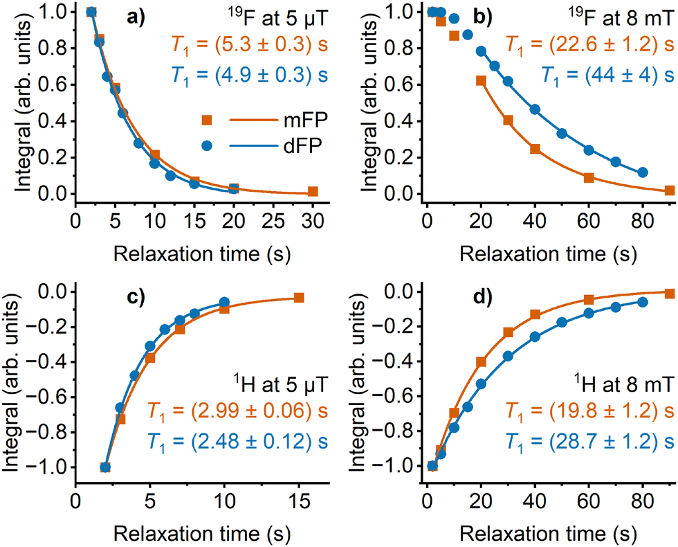Fig. 8 Relaxation time analysis of SABRE-hyperpolarised ¹⁹F and ¹H nuclei at selected magnetic fields. ¹⁹F at (a) 5 μT and (b) 8 mT. ¹H at (c) 5 μT and (d) 8 mT.

Table 1 T ₁ relaxation time constants for SABRE-hyperpolarised ¹⁹F and ¹H nuclei in mFP and dFP

Relaxation field	T 1 (mFP, ^19F) (s)	T 1 (mFP, ^1H) (s)	T 1 (dFP, ^19F) (s)	T 1 (dFP, ^1H) (s)
5 μT	5.3 ± 0.3	2.99 ± 0.06	4.9 ± 0.3	2.48 ± 0.12
50 μT	13.0 ± 0.2	14.1 ± 0.2	15.4 ± 0.8	17.9 ± 0.8
0.5 mT	16.2 ± 0.4	19.9 ± 0.5	16.1 ± 0.7	26.8 ± 1.3
8 mT	22.6 ± 1.2	19.8 ± 1.2	44 ± 4	28.7 ± 1.2
1 T	16.3 ± 0.6	19.2 ± 0.3	19.1 ± 0.5	36.0 ± 0.6

---

The results indicate an obvious trend: regardless of the substrate or nucleus under study, the relaxation time is significantly shortened when the sample is placed at an ultralow field. For ¹⁹F, the relaxation time T₁ ∼ 5 s is found, whereas for ¹H the relaxation is even faster, with T₁ ∼ 3 s. This raises an important technical aspect regarding the applications of SABRE-SHEATH. Once the sample has been hyperpolarised at an ultralow field, it is important to quickly change the magnetic field, not to lose the polarisation.

It is commonly known that scalar relaxation of the second kind (SRSK), which is operative when the nucleus under study is scalar-coupled to a rapidly-relaxing quadrupolar nucleus, can provide a very efficient relaxation mechanism, especially at weak magnetic fields.^39,40 Therefore, another option for lengthening the relaxation time would be to use isotopically enriched substrate, in which the quadrupolar ¹⁴N were replaced with ¹⁵N. Indeed, Birchall et al.⁴¹ have shown that the presence of the quadrupolar ¹⁴NO₂ site in metronidazole leads to a 3-fold decrease in the T₁ relaxation time of a neighbouring ¹⁵N centre in the SABRE-SHEATH regime. At high field (1.4 T), the difference between the samples with and without ¹⁴N was, however, insignificant. The negative impact of quadrupolar ¹⁴N has also been reported for ¹³C by Barskiy et al.⁴² There are not many experimental results of the effect of quadrupolar ¹⁴N on fluoropyridines. However, Chukanov et al.²⁸ compared the efficiency of SABRE hyperpolarisation between ¹⁴N-mFP and ¹⁵N-mFP, and reported similar ¹⁹F polarisation levels for the two isotopomers.

In the present measurements, a significant deviation from the general trend is observed for ¹⁹F at 8 mT: after the sample has been hyperpolarised, relaxation does not give rise to a single-exponential magnetisation decay, as is evident from Fig. 8(b). A significant factor behind this is that, for relaxation studies at 8 mT, ¹⁹F was hyperpolarised at 8 mT. This means that the ¹H centres were also substantially polarised and the hyperpolarisation of ¹⁹F was mostly obtained via cross-relaxation from ¹H. Hence, the polarisation transfer process from ¹H to ¹⁹F remains active for some time even after the pH₂ flow has been terminated. Because of this, the exponential fit was only applied to data points from 20 s onwards. Nevertheless, the obtained T₁ values were longer in comparison to values at both 0.5 mT and 1 T, especially for dFP. Similar findings have been reported by Kabir et al. at μT-fields, where the spin-relay process from ¹⁵N to ¹⁹F significantly lengthened the effective T₁ of the ¹⁹F nuclei.³⁵ Another consequence of this phenomenon is that the existence of efficient polarisation transfer to another nucleus within a substrate, especially via the spin-relay mechanism, may limit the observable polarisation of the first nucleus. This is particularly true in the cases where the second nucleus has a short T₁ and, therefore, acts as a polarisation sink.

4.4 Build-up times

The build-up times, T_b, of ¹⁹F and ¹H SABRE hyperpolarisation in mFP and dFP were determined by fitting eqn (1) to the datasets. The obtained fits, together with the build-up time constants, are collected in Fig. 9.

Fig. 9 Determination of SABRE hyperpolarisation build-up times for ¹⁹F and ¹H nuclei in mFP and dFP at different magnetic fields. ¹⁹F at (a) 5 μT and (b) 8 mT. ¹H at (c) 5 μT and (d) 8 mT.

The build-up time constants and their comparison to relaxation time constants provide useful information about the possible limiting factors in the polarisation transfer process. From Fig. 9(a) it is found that the ¹⁹F nuclei exhibit a quick build-up process with T_b ∼ 4 s at 5 μT. The fact that T_b is comparable to T₁ at this field (∼5 s) implies that the maximum achievable polarisation level is strongly limited by relaxation. This is also one of the reasons behind the smaller levels of polarisation obtained for ¹⁹F compared to ¹H in our study. Similar findings have been made in the cases of other heteronuclei, such as ¹⁵N and ¹³C, in earlier work.^{6,8–10,21,41–44}

When the polarisation transfer field is raised to 8 mT, the build-up of ¹⁹F polarisation becomes significantly longer (28 s for mFP and 41 s for dFP), as shown in Fig. 9(b). Even though the build-up process at mT-fields is complex due to its relayed nature, the build-up constants T_b are again comparable to the relaxation time constants T₁. When comparing the build-up time constants for ¹⁹F and ¹H at 8 mT [see Fig. 9(b) and (d)], the ¹⁹F polarisation is generated more slowly, consolidating the picture of relayed polarisation transfer via¹H.

The ¹H nuclei do not become significantly hyperpolarised at 5 μT, leading to ambiguity in the exponential fits to the data points shown in Fig. 9(c). There are also several polarisation transfer mechanisms that are operational for ¹H at the μT range fields, as well as distinct ¹H sites with different optimal polarisation transfer fields, varying lineshapes, and signs, as previously discussed for the PTF profiles.

Overall, the build-up time constants and the relaxation time constants are consistent with each other: short T_b is associated with short T₁ and vice versa. The conclusion is that the efficiency of SABRE hyperpolarisation is generally limited by relaxation.

5 Conclusions

In this work, SABRE experiments and spin dynamics simulations including chemical exchange and first-principles relaxation (Redfield theory) were used to characterise polarisation transfer to 3-monofluoropyridine (mFP) and 3,5-difluoropyridine (dFP). It is shown experimentally that the most efficient polarisation transfer to ¹⁹F nuclei occurs at the magnetic field of 5 μT, resulting in polarisation levels of 0.67% for mFP and 0.13% for dFP. This is verified with the simulations to be primarily due to coherent polarisation transfer, but the shape of the field dependence profile is strongly influenced also by the incoherent processes and these need to be incorporated into simulations to obtain reasonable compatibility with experiments. Particularly, the quadrupolar nuclei of the spin system can lead to large deviations between the theoretical and experimental results if incoherent mechanisms are neglected.

The coherent mechanism is also responsible for the optimum polarisation transfer to ¹H, leading to polarisation levels of −1.7% for mFP and −0.46% for dFP at 8 mT. In addition, relatively high ¹⁹F polarisation levels of 0.25% for mFP and 0.09% for dFP are observed at 8 mT. The spin dynamics simulations demonstrate that the polarisation transfer to ¹⁹F at mT fields mainly takes place incoherently through cross-relaxation from the ligand protons, which are first hyperpolarised coherently. The current simulations qualitatively reproduce the experimental results and give valuable insight into the mechanisms behind the polarisation transfer. However, a more accurate exchange model, which also takes into account the processes during the bubbling time, would be needed to obtain a quantitative description.

Author contributions

J. E. formal analysis, investigation, methodology, visualisation, writing – original draft. S. K.-M. S. formal analysis, investigation, methodology, software, writing – original draft. N. H. investigation, writing – review & editing. V. V. Z. resources, funding acquisition, writing – review & editing. J. V. conceptualisation, methodology, supervision, funding acquisition, writing – review & editing. A. M. K. conceptualisation, methodology, supervision, funding acquisition, writing – review & editing.

Data availability

Data for this article, including SpinSolve and Bruker spectrometer files, Turbomole input and output files, and spin dynamics simulation results with example script, are available at Fairdata Etsin at https://doi.org/10.23729/fd-076e04d7-3a0b-39bb-8b3b-0359b23bf582. Additional figures and analysis supporting this article have also been included as a ESI† to this article.

Conflicts of interest

There are no conflicts to declare.

Acknowledgements

The authors wish to thank Prof. Ilya Kuprov (Weizmann Institute of Science) for advice on the use of the Spinach code and Mr Eetu Hyypiö (Oulu) for writing the initial versions of the Matlab scripts used presently. We acknowledge funding from the Research Council of Finland (grants 351357, 331008, 361326, 362959) and U. Oulu (Kvantum Institute). Funding from Ruth and Nils-Erik Stenbäck foundation is appreciated (S. K.-M. S.). The experimental work was carried out in the NMR laboratory of the Centre for Material Analysis, University of Oulu, Finland. Computations were carried out at CSC – the Finnish IT centre for Science and the Finnish Grid and Cloud Infrastructure project (persistent identifier urn:nbn:fi:researchinfras-2016072533).

Notes and references

1. R. W. Adams, J. A. Aguilar, K. D. Atkinson, M. J. Cowley, P. I. P. Elliott, S. B. Duckett, G. G. R. Green, I. G. Khazal, J. López-Serrano and D. C. Williamson, Science, 2009, 323, 1708–1711.
2. K. D. Atkinson, M. J. Cowley, P. I. P. Elliott, S. B. Duckett, G. G. R. Green, J. López-Serrano and A. C. Whitwood, J. Am. Chem. Soc., 2009, 131, 13362–13368.
3. R. W. Adams, S. B. Duckett, R. A. Green, D. C. Williamson and G. G. R. Green, J. Chem. Phys., 2009, 131, 194505.
4. M. J. Cowley, R. W. Adams, K. D. Atkinson, M. C. R. Cockett, S. B. Duckett, G. G. R. Green, J. A. B. Lohman, R. Kerssebaum, D. Kilgour and R. E. Mewis, J. Am. Chem. Soc., 2011, 133, 6134–6137.
5. W. Iali, S. S. Roy, B. J. Tickner, F. Ahwal, A. J. Kennerley and S. B. Duckett, Angew. Chem., Int. Ed., 2019, 58, 10271–10275.
6. D. A. Barskiy, R. V. Shchepin, A. M. Coffey, T. Theis, W. S. Warren, B. M. Goodson and E. Y. Chekmenev, J. Am. Chem. Soc., 2016, 138, 8080–8083.
7. P. J. Rayner, M. J. Burns, A. M. Olaru, P. Norcott, M. Fekete, G. G. R. Green, L. A. R. Highton, R. E. Mewis and S. B. Duckett, Proc. Natl. Acad. Sci. U. S. A., 2017, 114, E3188–E3194.
8. M. Fekete, F. Ahwal and S. B. Duckett, J. Phys. Chem. B, 2020, 124, 4573–4580.
9. J. F. P. Colell, A. W. J. Logan, Z. Zhou, R. V. Shchepin, D. A. Barskiy, G. X. J. Ortiz, Q. Wang, S. J. Malcolmson, E. Y. Chekmenev, W. S. Warren and T. Theis, J. Phys. Chem. C, 2017, 121, 6626–6634.
10. T. Theis, M. L. Truong, A. M. Coffey, R. V. Shchepin, K. W. Waddell, F. Shi, B. M. Goodson, W. S. Warren and E. Y. Chekmenev, J. Am. Chem. Soc., 2015, 137, 1404–1407.
11. T. Theis, M. Truong, A. M. Coffey, E. Y. Chekmenev and W. S. Warren, J. Magn. Reson., 2014, 248, 23–26.
12. T. Theis, N. M. Ariyasingha, R. V. Shchepin, J. R. Lindale, W. S. Warren and E. Y. Chekmenev, J. Phys. Chem. Lett., 2018, 9, 6136–6142.
13. S. Knecht, A. S. Kiryutin, A. V. Yurkovskaya and K. L. Ivanov, Mol. Phys., 2019, 117, 2762–2771.
14. A. N. Pravdivtsev, N. Kempf, M. Plaumann, J. Bernarding, K. Scheffler, J.-B. Hövener and K. Buckenmaier, ChemPhysChem, 2021, 22, 2381–2386.
15. S. L. Eriksson, J. R. Lindale, X. Li and W. S. Warren, Sci. Adv., 2022, 8, eabl3708.
16. W. Iali, P. J. Rayner and S. B. Duckett, Sci. Adv., 2018, 4, eaao6250.
17. P. J. Rayner, J. P. Gillions, V. D. Hannibal, R. O. John and S. B. Duckett, Chem. Sci., 2021, 12, 5910–5917.
18. B. J. Tickner, M. Dennington, B. G. Collins, C. A. Gater, T. F. N. Tanner, A. C. Whitwood, P. J. Rayner, D. P. Watts and S. B. Duckett, ACS Catal., 2024, 14, 994–1004.
19. M. L. Truong, F. Shi, P. He, B. Yuan, K. N. Plunkett, A. M. Coffey, R. V. Shchepin, D. A. Barskiy, K. V. Kovtunov, I. V. Koptyug, K. W. Waddell, B. M. Goodson and E. Y. Chekmenev, J. Phys. Chem. B, 2014, 118, 13882–13889.
20. B. Erriah and S. J. Elliott, RSC Adv., 2019, 9, 23418–23424.
21. M. L. Truong, T. Theis, A. M. Coffey, R. V. Shchepin, K. W. Waddell, F. Shi, B. M. Goodson, W. S. Warren and E. Y. Chekmenev, J. Phys. Chem. C, 2015, 119, 8786–8797.
22. A. N. Pravdivtsev, F. Sönnichsen and J.-B. Hövener, J. Magn. Reson., 2018, 297, 86–95.
23. H. Hogben, M. Krzystyniak, G. Charnock, P. Hore and I. Kuprov, J. Magn. Reson., 2011, 208, 179–194.
24. A. Browning, K. Macculloch, P. TomHon, I. Mandzhieva, E. Y. Chekmenev, B. M. Goodson, S. Lehmkuhl and T. Theis, Phys. Chem. Chem. Phys., 2023, 25, 16446–16458.
25. R. V. Shchepin, B. M. Goodson, T. Theis, W. S. Warren and E. Y. Chekmenev, ChemPhysChem, 2017, 18, 1961–1965.
26. K. Buckenmaier, M. Rudolph, C. Back, T. Misztal, U. Bommerich, P. Fehling, D. Koelle, R. Kleiner, H. A. Mayer, K. Scheffler, J. Bernarding and M. Plaumann, Sci. Rep., 2017, 7, 13431.
27. A. M. Olaru, T. B. R. Robertson, J. S. Lewis, A. Antony, W. Iali, R. E. Mewis and S. B. Duckett, ChemistryOpen, 2018, 7, 97–105.
28. N. V. Chukanov, O. G. Salnikov, R. V. Shchepin, A. Svyatova, K. V. Kovtunov, I. V. Koptyug and E. Y. Chekmenev, J. Phys. Chem. C, 2018, 122, 23002–23010.
29. N. M. Ariyasingha, J. R. Lindale, S. L. Eriksson, G. P. Clark, T. Theis, R. V. Shchepin, N. V. Chukanov, K. V. Kovtunov, I. V. Koptyug, W. S. Warren and E. Y. Chekmenev, J. Phys. Chem. Lett., 2019, 10, 4229–4236.
30. A. I. Silva Terra, M. Rossetto, C. L. Dickson, G. Peat, D. Uhrín and M. E. Halse, ACS Meas. Sci. Au, 2023, 3, 73–81.
31. K. Sheberstov, E. Van Dyke, J. Xu, R. Kircher, L. Chuchkova, Y. Hu, S. Alvi, D. Budker and D. Barskiy, ChemRxiv, 2025, preprint DOI:10.26434/chemrxiv-2024-prw8k-v2.
32. A. N. Pravdivtsev, A. V. Yurkovskaya, H.-M. Vieth, K. L. Ivanov and R. Kaptein, ChemPhysChem, 2013, 14, 3327–3331.
33. A. N. Pravdivtsev, K. L. Ivanov, A. V. Yurkovskaya, P. A. Petrov, H.-H. Limbach, R. Kaptein and H.-M. Vieth, J. Magn. Reson., 2015, 261, 73–82.
34. R. V. Shchepin, L. Jaigirdar, T. Theis, W. S. Warren, B. M. Goodson and E. Y. Chekmenev, J. Phys. Chem. C, 2017, 121, 28425–28434.
35. M. S. H. Kabir, S. M. Joshi, A. Samoilenko, I. Adelabu, S. Nantogma, J. G. Gelovani, B. M. Goodson and E. Y. Chekmenev, J. Phys. Chem. A, 2023, 127, 5018–5029.
36. C. Bengs and M. H. Levitt, J. Magn. Reson., 2020, 310, 106645.
37. S. Knecht, A. S. Kiryutin, A. V. Yurkovskaya and K. L. Ivanov, J. Magn. Reson., 2018, 287, 74–81.
38. S. Knecht, S. Hadjiali, D. A. Barskiy, A. Pines, G. Sauer, A. S. Kiryutin, K. L. Ivanov, A. V. Yurkovskaya and G. Buntkowsky, J. Phys. Chem. C, 2019, 123, 16288–16293.
39. D. Kubica, A. Wodynski, A. Kraska-Dziadecka and A. Gryff-Keller, J. Phys. Chem. A, 2014, 118, 2995–3003.
40. S. J. Elliott, C. Bengs, L. J. Brown, J. T. Hill-Cousins, D. J. OLeary, G. Pileio and M. H. Levitt, J. Chem. Phys., 2019, 150, 064315.
41. J. R. Birchall, M. S. H. Kabir, O. G. Salnikov, N. V. Chukanov, A. Svyatova, K. V. Kovtunov, I. V. Koptyug, J. G. Gelovani, B. M. Goodson, W. Pham and E. Y. Chekmenev, Chem. Commun., 2020, 56, 9098–9101.
42. D. A. Barskiy, R. V. Shchepin, C. P. N. Tanner, J. F. P. Colell, B. M. Goodson, T. Theis, W. S. Warren and E. Y. Chekmenev, ChemPhysChem, 2017, 18, 1493–1498.
43. I. Adelabu, P. TomHon, M. S. H. Kabir, S. Nantogma, M. Abdulmojeed, I. Mandzhieva, J. Ettedgui, R. E. Swenson, M. C. Krishna, T. Theis, B. M. Goodson and E. Y. Chekmenev, ChemPhysChem, 2022, 23, e202100839.
44. R. V. Shchepin, D. A. Barskiy, A. M. Coffey, T. Theis, F. Shi, W. S. Warren, B. M. Goodson and E. Y. Chekmenev, ACS Sens., 2016, 1, 640–644.

---

Footnote

† Electronic supplementary information (ESI) available: Experimental details, modelling details, additional discussion of experimental results, and detailed simulation results. See DOI: https://doi.org/10.1039/d5cp01418b

---