
 Open Access Article
 This Open Access Article is licensed under a
 Creative Commons Attribution 3.0 Unported Licence
Modeling the projected range of protons in matter: insights from molecular dynamics and quantum chemistry†
Chieh-Min
Hsieh
 a,
Alexander
Dellwisch
a and
Tim
Neudecker
*abc
a,
Alexander
Dellwisch
a and
Tim
Neudecker
*abc
aUniversity of Bremen, Institute for Physical and Theoretical Chemistry, Leobener Str. 6, D-28359 Bremen, Germany. E-mail: neudecker@uni-bremen.de
bBremen Center for Computational Materials Science, Am Fallturm 1, D-28359 Bremen, Germany
cMAPEX Center for Materials and Processes, Bibliothekstr. 1, D-28359 Bremen, Germany
First published on 11th June 2025
Abstract
Estimating the projected range of high-energy particles is important for ion implantation and designing shielding strategies for space devices. In this work, we propose a molecular dynamics (MD) workflow to calculate the projected range of protons and demonstrate its capabilities by calculating the projected range of protons in graphite and poly(methyl methacrylate) (PMMA). The results show excellent agreement with reference data. Besides, we investigate irradiation-induced bond breaking by simulating the proton bombardment of a perylene-3,4,9,10-tetracarboxylic dianhydride (PTCDA) molecule and analyze the strain energy accumulated in the system using quantum chemical tools. The findings indicate a correlation between strain energy and the kinetic energy of the primary knock-on atom.
1. Introduction
Understanding how high-energy particles behave in matter is crucial, as it can lead to several important applications. One such example is ion implantation, a process that alters the properties of a target material by embedding accelerated ions into it.1–4 For instance, when silicon is implanted with boron or arsenic ions, it becomes a p-type or n-type semiconductor, which is fundamental in semiconductor device fabrication. Moreover, plenty of high-energy particles exist in space, such as protons, alpha particles, and high-energy electrons.5 These particles can damage materials in various ways, such as creating defect sites in crystals, breaking chemical bonds, forming blisters, and causing embrittlement in materials.6–8 Therefore, a proper shielding strategy must be employed to protect the materials from potential degradation caused by these high-energy particles. Consequently, estimating the projected range, which refers to the mean penetration depth of the projectiles in materials, is essential for space missions.One common approach to estimate the projected range is the binary collision approximation (BCA),9 which models the recoil event as a series of collisions between two particles. This method is effective and computationally efficient for simulating particle collisions. The widely used Stopping and Range of Ions in Matter (SRIM) code,10 based on the BCA and Monte Carlo11 approach, is a prominent example in this category. However, a limitation of this method is that it models the trajectories of particles only in amorphous materials. Later, molecular dynamics (MD) for calculating the projected range gained attention. A notable first attempt was the MDRANGE code,12 developed by Nordlund in the 1990s. Although MD is computationally more expensive than BCA, it models the crystal structures atomistically, enabling more accurate range prediction for crystalline materials. As a result, MD has successfully estimated the range of several crystalline materials, showing its potential in this field.13,14
Although the aforementioned methods have been effective, they were developed decades ago and have significant limitations, as they primarily target inorganic solids. For instance, polymers—important materials for space applications—may not be accurately analyzed using these methods due to their more complex chemical bonding patterns. In this paper, we revisit calculating the projected range of protons in matter using the state-of-the-art Large-scale Atomic/Molecular Massively Parallel Simulator (LAMMPS) MD code.15 Specifically, we employed MD to calculate the projected range of high-velocity protons in two chemically very diverse materials: graphite and poly(methyl methacrylate) (PMMA). The former has a stacked layer structure, while the latter is a polymer. For these simulations, we used the reactive force field (ReaxFF) potential,16 which includes elements commonly found in organic materials (e.g., H, C, O, and N) and is considered a well-established method for modeling bond rupture events in such systems. For both graphite and PMMA, which contain typical organic bonds (C![[double bond, length as m-dash]](https://www.rsc.org/images/entities/char_e001.gif) O, C–H, C–C, and aromatic structures), our use of ReaxFF yielded equilibrium densities in reasonable agreement with experimental values, supporting the validity of our chosen potential. Last but not least, we explored the degradation scenarios, such as bond breaking, and applied the quantum chemical Judgement of Energy DIstribution (JEDI) strain analysis17,18 to investigate the strain energy induced by the impacting proton in a single perylene-3,4,9,10-tetracarboxylic dianhydride (PTCDA) molecule.
O, C–H, C–C, and aromatic structures), our use of ReaxFF yielded equilibrium densities in reasonable agreement with experimental values, supporting the validity of our chosen potential. Last but not least, we explored the degradation scenarios, such as bond breaking, and applied the quantum chemical Judgement of Energy DIstribution (JEDI) strain analysis17,18 to investigate the strain energy induced by the impacting proton in a single perylene-3,4,9,10-tetracarboxylic dianhydride (PTCDA) molecule.
2. Computational approach
2.1. General considerations for high-velocity projectiles in MD
Compared to regular MD simulations, simulating high-velocity projectiles in materials requires specific setups. The stopping power S(E), for example, is a crucial parameter that is defined as the energy loss per unit penetration distance,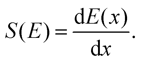 | (1) |
When a projectile interacts with atoms, the force acting between them is reduced by a friction force, as
 | (2) |
![[F with combining right harpoon above (vector)]](https://www.rsc.org/images/entities/i_char_0046_20d1.gif) i is the adjusted force, 0i is the original force between the projectile and an atom in the material, and
i is the adjusted force, 0i is the original force between the projectile and an atom in the material, and ![[v with combining right harpoon above (vector)]](https://www.rsc.org/images/entities/i_char_0076_20d1.gif) i is the velocity of the projectile.
i is the velocity of the projectile.
The other key parameter is the Ziegler–Biersack–Littmark (ZBL)19 repulsive interatomic potential, which is defined as
 | (3) |
 | (4) |
Finally, adaptive time steps are essential to make the time step inversely proportional to the projectile's velocity.20 This means that a shorter time step is applied when the projectile's velocity is high, while a longer time step is used when the projectile slows down. This approach ensures both the accuracy and efficiency of the calculation.
2.2. Projected range of protons
Since high-velocity protons penetrate deep into materials over large distances,21 it is impractical to simulate the entire process using MD with a sufficiently large simulation cell. To address this, Nordlund's approach12 shifts atoms when the projectile is near the boundary. Specifically, when the distance between the projectile and the boundary is smaller than Si, all atoms are shifted away from the boundary by a distance of Si. The space created by shifting atoms is then filled with new lattice atoms. This method ensures that the proton does not pass through the boundary and re-enters the simulation cell with a damaged lattice structure. While effective for crystalline materials, this approach is not suitable for non-crystalline materials, such as amorphous polymers.In our approach, the proton is initially placed at a random position at the boundary of the simulation cell with a specified initial velocity in the z-direction, as demonstrated in Fig. 1. An MD simulation is then initiated. During the simulation, the system evolves without a thermostat or barostat, and the temperature rises during the simulation, reflecting an adiabatic process where the proton deposits energy into the material over a short timescale. In our previous tests, applying NVT or NPT conditions in this step led to a significant underestimation of the proton's projected range. Simultaneously, the proton's kinetic energy is monitored until the simulation terminates under one of two conditions: (1) the proton reaches the boundary of the simulation cell again. In this situation, the proton's velocity is recorded and used to initialize a new MD simulation. (2) the proton's kinetic energy drops below 1 eV (indicating the proton is stopped). In this case, the simulation is done, and the projected range is determined as the sum of the penetration distances in the z-direction across all individual MD runs. The workflow of the simulation process is illustrated in Fig. 2.
 | ||
| Fig. 1 Initial stage of an MD simulation showing a proton (green) traveling through PMMA. The arrow indicates the direction of the assigned initial velocity. Color code: C (red), H (yellow), O (blue). | ||
 | ||
| Fig. 2 The MD workflow for simulating the projected range of a proton in a material. | ||
The MD simulations of the projected range were carried out using the LAMMPS code. Initially, the system was equilibrated using the NPT ensemble with a Nosé–Hoover thermostat22,23 and a Nosé–Hoover barostat with Martyna–Tuckerman–Klein (MTK) corrections24 at 50 K and 1 atm. A proton was then positioned at the boundary of the simulation cell on the xy-plane with its z-coordinate set to 0, while its x- and y-coordinate were assigned randomly. The proton was given an initial velocity corresponding to a kinetic energy of 1, 5, 10, 20, or 50 keV, directed along the negative z-direction. The simulation then proceeded by following the MD workflow (Fig. 2) to determine the projected range. For each initial proton kinetic energy value, 20 individual trajectories were calculated to obtain a statistically meaningful distribution.
Periodic boundary conditions were applied in all calculations. The ReaxFF potential (ffield.reax.FC)25,26 distributed with the LAMMPS code was used to model the systems, with the ReaxFF algorithm implemented in LAMMPS, as described in the corresponding reference.27 The ZBL19 potential with inner and outer cutoffs of 3.0 and 4.0 Å, respectively, was applied to account for the repulsive interactions between the projectile and the atoms within the target material. In addition, stopping power from the PSTAR database was employed to account for the inelastic energy loss of the proton during penetration. It should be noted that stopping powers below 1 keV are not available in the PSTAR database. Therefore, the stopping power provided by SRIM was used for this energy range. Finally, the time step was adjusted using the dt/reset command to limit the proton's maximum travel distance per simulation step to 0.005 Å, ensuring the time step was appropriately assigned.
To validate our simulation, we utilized the PSTAR database and the SRIM code as references. The PSTAR database is provided by the National Institute of Standards and Technology (NIST). It contains a stopping power table of protons, which is derived from a combination of experimental data and theoretical predictions based on the Bethe formula.28 This database also provides the projected range R, which is calculated by integrating the reciprocal stopping power over the energy range, as shown in
 | (5) |
SRIM calculations were performed using the 2013 version of the SRIM code.10 The ion was hydrogen with a mass of 1.008 amu. The graphite target consisted of carbon atoms with a density of 1.70 g cm−3, while the PMMA target was composed of hydrogen, carbon, and oxygen atoms in an atomic ratio of 8![[thin space (1/6-em)]](https://www.rsc.org/images/entities/char_2009.gif) :5:2, with a density of 1.18 g cm−3.
:5:2, with a density of 1.18 g cm−3.
2.3. Preparation of the material configurations
In our simulations, the graphite supercell was modeled using a hexagonal simulation cell with lattice parameters of 9.85 Å, 9.85 Å, and 26.84 Å, containing a total of 256 carbon atoms. The PMMA system under investigation contains 8 chains with 10 monomers each. The structure was generated using the Polymer Modeler tool,29 which randomly placed syndiotactic PMMA polymer chains in a cubic simulation cell. The initial packing density was deliberately set to a low value of 0.5 g cm−3. Moltemplate30 was used as a preprocessing tool to create the necessary data files. The subsequent equilibration was conducted using the LAMMPS code. Interatomic forces were calculated using the OPLS-AA force field.31 Newtons equations of motion were integrated using the velocity Verlet algorithm32 with a time step of 1 fs. Periodic boundary conditions were implemented in all directions, and the PPPM Ewald summation method33 was used to compute long-range electrostatic interactions with a neighboring list cutoff set to 12 Å.To increase the density, an NPT run using Nosé–Hoover thermostat and Nosé–Hoover barostat with MTK corrections was performed at 300 K and 1 atm for 0.5 ns. This was followed by a 21-step relaxation procedure34 for enhanced equilibration, involving various compression and decompression steps within a pressure range of 1 to 50000 atm and a temperature range of 300 to 1000 K over a total simulation time of 1.56 ns. This 21-step equilibration process has been used for the preparation of various systems in the past.35–37 During equilibration, the simulation cell was resized, resulting in a density of 1.11 g cm−3, which is close to the experimental value of 1.17 g cm−3.38 The equilibrated system obtained from the 21-step equilibration procedure was then used as the initial configuration for calculating the projected range.
2.4. PTCDA molecule bombarded by a proton
A PTCDA molecule was positioned at the center of a rectangular simulation box with dimensions 21.5 × 16.8 × 30 Å. A proton was placed 13.5 Å above the molecule, with its initial velocity directed toward the molecule, as shown in Fig. 3. To consider all impact positions, a two-dimensional scan with a resolution of 0.1 Å was performed, covering a 6 × 4 Å area. In this MD simulation, the ReaxFF potential was utilized to describe the chemical bonds within the molecule, while the ZBL potential was used to account for collisions between the proton and target atoms. The ZBL cutoff distances were set to 3.0 Å (inner) and 4.0 Å (outer). Periodic boundary conditions were applied in the x- and y-directions, while the z-direction was kept non-periodic to prevent the proton from re-entering the simulation box. The time step was controlled using the dt/reset command, which limited the maximum distance traveled by the proton during each simulation step to 0.003 Å. Finally, the bond distances were evaluated at the end of the simulation. If a bond distance exceeded 1.3 times the sum of the covalent radii, the bond was considered broken. | ||
| Fig. 3 A PTCDA molecule with the highlighted rectangular area indicating the region impacted by the proton. | ||
2.5. JEDI strain analysis
We utilized the Judgement of Energy DIstribution (JEDI) strain analysis tool,17,18 implemented in the Atomic Simulation Environment (ASE),39 to analyze the strain induced by an impacting proton on a PTCDA molecule. A geometry optimization and a frequency calculation based on density functional theory (DFT) were performed to obtain the Hessian matrix of the PTCDA molecule in redundant internal coordinates (RICs). These tasks were carried out using the Vienna Ab initio Simulation Package (VASP).40 The starting geometry was the same as in Section 2.4, but without the proton. A plane-wave basis set with pseudo potentials was used to describe the electronic structure, with an energy cutoff of 500 eV applied for the plane-wave basis set. The PBE41 density functional was employed, and the Grimme DFT-D3 dispersion correction with the Becke–Johnson damping42 function was included in the calculations. The distorted structures were snapshots taken from the proton bombardment MD simulations described in Section 2.4. Using the Hessian matrix, the JEDI code calculated the strain energy based on the deviation of internal coordinates between distorted and strain-free structures during the MD trajectories.3. Results and discussion
3.1. Projected range of protons in materials
Compared to reference data from SRIM and the PSTAR database, our MD results generally exhibit remarkable agreement, as presented in Table 1. However, for graphite at lower kinetic energies (up to 10 keV), the deviation from SRIM is relatively large, reaching up to 19%. Furthermore, the results for PMMA also show significant deviations from SRIM, as high as 26%. These deviations are highlighted in the plot shown in Fig. 4.| 1 keV | 5 keV | 10 keV | 20 keV | 50 keV | |
|---|---|---|---|---|---|
| Graphite | |||||
| Avg. MD range | 182 | 793 | 1314 | 2472 | 4994 |
| SD | 57 | 175 | 297 | 424 | 409 |
| SRIM range | 220 | 933 | 1630 | 2745 | 5385 |
| PSTAR range | 179 | 837 | 1502 | 2602 | 5237 |
| Dev. from SRIM range | −17% | −15% | −19% | −10% | −7% |
| Dev. from PSTAR range | 2% | −5% | −13% | −5% | −5% |
| PMMA | |||||
| Avg. range | 225 | 876 | 1616 | 2958 | 5727 |
| SD | 70 | 264 | 263 | 220 | 415 |
| SRIM range | 281 | 1188 | 2065 | 3450 | 6668 |
| PSTAR range | 224 | 1026 | 1809 | 3074 | 6092 |
| Dev. from SRIM range | −20% | −26% | −22% | −14% | −14% |
| Dev. from PSTAR range | 0% | −15% | −11% | −4% | −6% |
 | ||
| Fig. 4 Comparison of the projected range of protons in graphite and PMMA calculated in this study with reference data from PSTAR and SRIM. Error bars represent one standard deviation. | ||
To investigate this discrepancy, we compared the stopping power of the two materials, defined as the proton's energy loss per unit penetration distance (eqn (1)), as provided by SRIM and PSTAR. As illustrated in Fig. 5, the stopping power for PMMA obtained from PSTAR is slightly higher than that from SRIM. This difference is expected to result in a smaller calculated projected range when the stopping power from PSTAR is used. It is important to note that our calculations combined the stopping power data from both PSTAR and SRIM. Specifically, for the kinetic energy values from 1 keV to 50 keV, the stopping power was taken from PSTAR, while for kinetic energy values below 1 keV, the stopping power was obtained from SRIM, as PSTAR does not provide data for this range. This leads to a larger calculated range, especially for calculations with a low-energy proton. As seen in the trend of the blue curve in Fig. 4—when compared to the red and green curves—we observed that the data points for graphite at 1 and 5 keV, as well as PMMA at 1 keV, are higher than expected. This anomaly can be attributed to the lower stopping power from SRIM, which leads to a larger calculated projected range.
 | ||
| Fig. 5 Comparison of the stopping power of protons in graphite and PMMA over the kinetic energy range of 1 keV to 100 keV. | ||
It is worth mentioning that, during the simulation, the proton can change its direction, indicating the proton collided with an atom in the material and rebounded in a different direction. This behavior can be attributed to the repulsive force generated by the incorporated ZBL potential, which is crucial for decelerating the proton. In our preliminary calculations, we observed that without the ZBL potential, the projected range of the proton was highly overestimated.
Moreover, we conducted five additional simulations for graphite with proton energies of 1 keV and 5 keV, respectively. Our results indicate that the energy loss due to electronic stopping is trajectory-dependent. For 1 keV protons, the fraction of kinetic energy lost to electronic stopping ranges from 54% to 70%, whereas for 5 keV protons, this increases to 83% to 92%. This trend is expected, as higher-energy protons travel farther and interact with more electrons, resulting in greater cumulative energy loss via electronic stopping. In contrast, lower-energy protons undergo more frequent nuclear collisions, which contribute more significantly to nuclear stopping—that is, energy loss due to repulsive interactions described by the ZBL potential.
In conclusion, the overall satisfactory results lend credibility to our simulation approach, and this opens up the possibility to simulate the projected range of protons in a wide range of organic materials in the future.
3.2. Degradation of molecules
Shi et al.43 applied classical MD to simulate defect generation in graphene bombarded by a proton. Specifically, they employed the Tersoff44 potential combined with the ZBL potential. They compared their MD results with ab initio MD (AIMD) simulations and observed consistency. In our study, we adopted a similar approach but used the ReaxFF potential instead of the Tersoff potential due to its greater compatibility with diverse atom types. Since both Tersoff and ReaxFF are bond-order potentials, they are well-suited for modeling bond breaking in MD simulations.
We conducted an MD simulation of a proton impacting a PTCDA molecule, which, similar to graphene, has a two-dimensional layered structure with a π-conjugated system. Besides, it contains hydrogen and oxygen atoms, which are common in organic compounds. The initial kinetic energy of the proton was set to 1 and 10 keV. Given the D2h symmetry of PTCDA, only one-fourth of the impact area needed to be analyzed. To thoroughly evaluate the whole impact region, a two-dimensional scan with a resolution of 0.1 Å in the xy-plane was performed, as illustrated in Fig. 3.
The results of bond breaking analysis suggest that the impact position must be close to the primary knock-on atom (PKA) to break bonds, as illustrated in Fig. 6, where the red circles (bond breaking occurs) align with the nuclear configuration of a PTCDA molecule. This observation is consistent with the findings of Shi et al.43 Besides, the number of red circles demonstrates the stability of the corresponding atom. For instance, the carbon atoms in the aromatic ring of the perylene core are more stable than the carbon atom in the carboxylic anhydride group. Moreover, as the proton's kinetic energy increases, the number of red circles decreases, implying a reduced probability of bond breaking. This trend arises because higher-energy protons have a shorter interaction time to transfer energy to the PKA.43
 | ||
| Fig. 6 MD simulation results of proton bombardment on a PTCDA molecule. Position (0, 0) represents the center of the PTCDA molecule. Each circle marks an impacting position, with red circles denoting bond breaking events. | ||
We also analyzed the maximum kinetic energy of the PKA during our simulations for different impact positions. As shown in Fig. 7, a comparison of the kinetic energy of the PKA for bond-breaking and non-bond-breaking cases reveals a significant energy difference, confirming that the energy transferred to the PKA is decisive in damaging chemical bonds.
 | ||
| Fig. 7 MD simulation results showing the maximum kinetic energy of the PKA in the highlighted area of Fig. 6, expressed in kcal mol−1. | ||
Fig. 8 presents the MD snapshots of the PTCDA molecule just before the C–C bond breaking, with a color scale highlighting the strain energy distribution. The analysis reveals that the strain energy is highly localized near the impact position. The strain energy stored in the C–C bond before bond breaking amounts to 96 kcal mol−1. Considering the resonance structure of the aromatic ring, the C–C bond strength should lie between a C–C single bond (ethane, 90 kcal mol−1) and a CC double bond (ethylene, 174 kcal mol−1).45 Although the strain energy calculated by JEDI falls within this range, the value appears to be slightly lower than expected. In cases where bond rupture did not occur, the strain energy was redistributed throughout the entire molecule, resulting in molecular vibrations. Videos demonstrating the dynamic strain energy distribution are available in the ESI.†
 | ||
| Fig. 8 Snapshots of the PTCDA molecule just before bond breaking induced by the impacting proton. The red dotted circle highlights the PKA, and the red arrow indicates the bond at the critical point of rupture. The colors of the bonds show the strain energy distribution as calculated by the JEDI analysis, resulting from the change in bond lengths, bond angles, and dihedral angles of the molecule. | ||
Furthermore, we compared the maximum strain energy of the distorted PTCDA molecule and the maximum kinetic energy of the PKA during the MD simulation, as demonstrated in Table 2. The maximum strain energy was determined for each impact position by analyzing the geometry of the PTCDA molecule in each MD trajectory using JEDI. The strain energies for four of the MD trajectories could not be calculated because the JEDI strain analysis is based on the harmonic approximation, which becomes invalid when bond breaking occurs. For the remaining cases, the kinetic energy value correlates with the strain energy, indicating that the kinetic energy of the PKA is converted into strain energy within the distorted structure. However, some relatively higher deviations are observed, which could be attributed to differences in bond length estimated by the ReaxFF potential compared to DFT calculations underlying the JEDI analyses. In addition, the following points need to be kept in mind: (1) the harmonic approximation used in JEDI generally leads to an underestimation of strain energy in compressive cases and an overestimation in stretching cases.18 (2) In dynamic JEDI, only potential energy is quantified; the contribution of kinetic energy of the strained system is neglected, and the relative contributions of each component remain unknown.17 (3) Strain induced by thermal vibrations may also contribute to the total strain of the molecular system. Combined, these effects explain the deviations between the kinetic energy of the proton and the strain energy of the system calculated with JEDI.
| 6–14 | 7–14 | 8–14 | 9–14 | |
|---|---|---|---|---|
| max.ke.PKA | 108 | 265 | 246 | 94 |
| max.strain | 105 | 249 | 239 | 112 |
| Dev. | −3% | −6% | −3% | 19% |
| 6–13 | 7–13 | 8–13 | 9–13 | |
|---|---|---|---|---|
| max.ke.PKA | 236 | 1834 | 1394 | 191 |
| max.strain | 181 | — | — | 164 |
| Dev. | −23% | — | — | −14% |
| 6–12 | 7–12 | 8–12 | 9–12 | |
|---|---|---|---|---|
| max.ke.PKA | 198 | 974 | 816 | 164 |
| max.strain | 171 | — | — | 151 |
| Dev. | −14% | — | — | −8% |
| 6–11 | 7–11 | 8–11 | 9–11 | |
|---|---|---|---|---|
| max.ke.PKA | 79 | 159 | 150 | 70 |
| max.strain | 103 | 145 | 146 | 106 |
| Dev. | 30% | −9% | −3% | 51% |
4. Conclusion and outlook
We have proposed an MD workflow that successfully simulates the projected range of protons in graphite and PMMA. Our approach demonstrates versatility, as it can be applied across various types of materials due to the generality of the ReaxFF potential. This is particularly notable for polymers, which are rarely considered in calculations of the projected range.Our JEDI strain analysis indicates that the strain induced by the proton is highly localized, and concentrated near the impact position. The strain energy is then redistributed throughout the molecule if the bond rupture does not occur, leading to increased atomic oscillations and, ultimately, heating of the system. Additionally, by comparing the kinetic energy of PKAs and the strain of the distorted PTCDA molecule, we conclude that most of the PKA's kinetic energy is converted into strain energy.
In our simulations, the proton is treated as a neutral particle, which is a simplified approximation. While this assumption has minimal influence on the calculated projected range, it may affect the material in other ways. For example, it could impact proton diffusion and the generation of radicals within the structure.46,47 To address this limitation, the accuracy provided by quantum mechanics (QM) is desirable. We see the potential of the electron force field (EFF) method as a solution to this issue.48,49 This method approximates quantum effects through the quantum wave packet, thereby providing a more accurate description of the electronic structure. Another promising approach is using machine learning force field (MLFF) potentials,50 which could enhance accuracy while maintaining the computational efficiency of classical MD simulations.
Conflicts of interest
The authors declare no conflicts of interest.Data availability
The data supporting this article are provided in the ESI.†Acknowledgements
We acknowledge funding from the Federal State of Bremen and the University of Bremen through the APF project ‘Materials on Demand’ within the ‘Humans on Mars' initiative. AD gratefully acknowledges funding by the Fonds der Chemischen Industrie. Also, we appreciate our colleagues Erik Klein, Dr Patric Seefeldt, Dr Maciej Sznajder, Tanja Link, Dr Katharina Koschek, and PD Dr Michael Maas for the inspiring and fruitful discussion. We also thank David Anbeh (University of Bremen) for running preliminary calculations. Their involvement in this project is invaluable to our work.References
- H. Ryssel and K. Hoffmann, Ion Implantation, Springer, 1983 Search PubMed.
- J. Williams, Mater. Sci. Eng.: A, 1998, 253, 8–15 CrossRef.
- M. A. Nastasi and J. W. Mayer, Ion Implantation and Synthesis of Materials, Springer, 2006, vol. 5 Search PubMed.
- J. F. Ziegler, Ion Implantation Science and Technology, Elsevier, 2012 Search PubMed.
- P. D. Group, P. Zyla, R. Barnett, J. Beringer, O. Dahl, D. Dwyer, D. Groom, C.-J. Lin, K. Lugovsky and E. Pianori, et al. , Prog. Theor. Exp. Phys., 2020, 083C01 CrossRef.
- K. Nordlund, S. J. Zinkle, A. E. Sand, F. Granberg, R. S. Averback, R. E. Stoller, T. Suzudo, L. Malerba, F. Banhart and W. J. Weber, et al. , J. Nucl. Mater., 2018, 512, 450–479 CrossRef CAS.
- K. Nordlund, J. Nucl. Mater., 2019, 520, 273–295 CrossRef CAS.
- M. Sznajder, U. Geppert and M. R. Dudek, npj Mater. Degrad., 2018, 2, 3 CrossRef.
- M. T. Robinson, Radiat. Eff. Defects Solids, 1994, 130, 3–20 CrossRef.
- J. F. Ziegler, M. D. Ziegler and J. P. Biersack, Nucl. Instrum. Methods Phys. Res., Sect. B, 2010, 268, 1818–1823 CrossRef CAS.
- F. James, Rep. Prog. Phys., 1980, 43, 1145 CrossRef CAS.
- K. Nordlund, Comput. Mater. Sci., 1995, 3, 448–456 CrossRef CAS.
- J. Peltola, K. Nordlund and J. Keinonen, Nucl. Instrum. Methods Phys. Res., Sect. B, 2002, 195, 269–280 CrossRef CAS.
- H. Chan, M. Srinivasan, N. Montgomery, C. Mulcahy, S. Biswas, H.-J. Gossmann, M. Harris, K. Nordlund, F. Benistant and C. Ng, et al. , J. Vac. Sci. Technol., B, 2006, 24, 462–467 CrossRef CAS.
- A. P. Thompson, H. M. Aktulga, R. Berger, D. S. Bolintineanu, W. M. Brown, P. S. Crozier, P. J. In't Veld, A. Kohlmeyer, S. G. Moore and T. D. Nguyen, et al. , Comput. Phys. Commun., 2022, 271, 108171 CrossRef CAS.
- A. C. Van Duin, S. Dasgupta, F. Lorant and W. A. Goddard, J. Phys. Chem. A, 2001, 105, 9396–9409 CrossRef CAS.
- T. Stauch and A. Dreuw, J. Chem. Phys., 2014, 140, 134107 CrossRef PubMed.
- H. Wang, S. Benter, W. Dononelli and T. Neudecker, J. Chem. Phys., 2024, 160, 152501 CrossRef CAS PubMed.
- J. F. Ziegler and J. P. Biersack, Treatise on Heavy-ion Science: Volume 6: Astrophysics, Chemistry, and Condensed Matter, Springer, 1985, pp. 93–129 Search PubMed.
- R. Smith and D. Harrison Jr, Comput. Phys., 1989, 3, 68–73 CrossRef.
- M. O. Burrell, The Calculation of Proton Penetration and Dose Rates, Nasa Technical Report, 1964 Search PubMed.
- S. Nosé, J. Chem. Phys., 1984, 81, 511–519 CrossRef.
- W. G. Hoover, Phys. Rev. A, 1985, 31, 1695 CrossRef PubMed.
- G. J. Martyna, D. J. Tobias and M. L. Klein, J. Chem. Phys., 1994, 101, 10–1063 CrossRef.
- K. Chenoweth, A. C. Van Duin and W. A. Goddard, J. Phys. Chem. A, 2008, 112, 1040–1053 CrossRef CAS PubMed.
- S. K. Singh, S. G. Srinivasan, M. Neek-Amal, S. Costamagna, A. C. Van Duin and F. Peeters, Phys. Rev. B, 2013, 87, 104114 CrossRef.
- H. M. Aktulga, J. C. Fogarty, S. A. Pandit and A. Y. Grama, Parallel Comput., 2012, 38, 245–259 CrossRef.
- H. Bethe, Ann. Phys., 1930, 397, 325–400 CrossRef.
- B. P. Haley, C. Li, N. Wilson, E. Jaramillo and A. Strachan, arXiv preprint, 2015, preprint, arXiv:1503.03894 Search PubMed.
- A. I. Jewett, D. Stelter, J. Lambert, S. M. Saladi, O. M. Roscioni, M. Ricci, L. Autin, M. Maritan, S. M. Bashusqeh and T. Keyes, et al. , J. Mol. Biol., 2021, 433, 166841 CrossRef CAS PubMed.
- W. L. Jorgensen, D. S. Maxwell and J. Tirado-Rives, J. Am. Chem. Soc., 1996, 118, 11225–11236 CrossRef CAS.
- W. C. Swope, H. C. Andersen, P. H. Berens and K. R. Wilson, J. Chem. Phys., 1982, 76, 637–649 CrossRef CAS.
- R. W. Hockney and J. W. Eastwood, Computer Simulation Using Particles, CRC Press, 2021 Search PubMed.
- L. J. Abbott, K. E. Hart and C. M. Colina, Theor. Chem. Acc., 2013, 132, 1–19 Search PubMed.
- M. Laurien, B. Demir, H. Buttemeyer, A. S. Herrmann, T. R. Walsh and L. Colombi Ciacchi, Macromolecules, 2018, 51, 3983–3993 CrossRef CAS.
- S. Kumar, B. Demir, A. Dellwisch, L. Colombi Ciacchi and T. Neudecker, Macromolecules, 2023, 56, 8438–8447 CrossRef CAS.
- S. Chakraborty, F. C. Lim and J. Ye, J. Phys. Chem. C, 2019, 123, 23995–24006 CrossRef CAS.
- W. Gall and N. McCrum, J. Polym. Sci., 1961, 50, 489–495 CrossRef CAS.
- A. H. Larsen, J. J. Mortensen, J. Blomqvist, I. E. Castelli, R. Christensen, M. Dułak, J. Friis, M. N. Groves, B. Hammer and C. Hargus, et al. , J. Phys.: Cond. Matter., 2017, 29, 273002 CrossRef PubMed.
- G. Kresse and J. Furthmüller, Phys. Rev. B: Condens. Matter Mater. Phys., 1996, 54, 11169 CrossRef CAS PubMed.
- J. P. Perdew, K. Burke and M. Ernzerhof, Phys. Rev. Lett., 1996, 77, 3865 CrossRef CAS PubMed.
- S. Grimme, S. Ehrlich and L. Goerigk, J. Comput. Chem., 2011, 32, 1456–1465 CrossRef CAS PubMed.
- T. Shi, Q. Peng, Z. Bai, F. Gao and I. Jovanovic, Nanoscale, 2019, 11, 20754–20765 RSC.
- J. Tersoff, Phys. Rev. B: Condens. Matter Mater. Phys., 1989, 39, 5566 CrossRef PubMed.
- J. McMurry, Organic Chemistry: A Tenth Edition, OpenStax, Rice University, 2023 Search PubMed.
- J. A. LaVerne, Z. Chang and M. Araos, Radiat. Phys. Chem., 2001, 60, 253–257 CrossRef CAS.
- R. Huszank, S. Z. Szilasi and D. Szikra, J. Phys. Chem. C, 2013, 117, 25884–25889 CrossRef CAS.
- J. T. Su and W. A. Goddard III, Phys. Rev. Lett., 2007, 99, 185003 CrossRef PubMed.
- A. Jaramillo-Botero, J. Su, A. Qi and W. A. Goddard III, J. Comput. Chem., 2011, 32, 497–512 CrossRef CAS PubMed.
- O. T. Unke, S. Chmiela, H. E. Sauceda, M. Gastegger, I. Poltavsky, K. T. Schutt, A. Tkatchenko and K.-R. Müller, Chem. Rev., 2021, 121, 10142–10186 CrossRef CAS PubMed.
Footnote |
| † Electronic supplementary information (ESI) available: Scripts for calculating the projected range of protons using LAMMPS, scripts for modeling proton bombardment on a PTCDA molecule, and videos showing dynamic strain distribution in the PTCDA molecule under proton bombardment are available. See DOI: https://doi.org/10.1039/d5cp00223k |
| This journal is © the Owner Societies 2025 |