A robust signal processing program for nanopore signals using dynamic correction threshold with compatible baseline fluctuations

Abstract

Solid-state nanopores represent a powerful platform for the detection and characterization of a wide range of biomolecules and particles, including proteins, viruses, and nanoparticles, for clinical and biochemical applications. Typically, nanopores operate by measuring transient pulses of ionic current during translocation events of molecules passing through the pore. Given the strong noise and stochastic fluctuations in ionic current recordings during nanopore experiments, signal processing based on the statistical analysis of numerous translocation events remains a crucial issue for nanopore sensing. Based on parallel computational processing and efficient memory management, we developed a novel signal processing procedure for translocation events to improve the signal identification performance of solid-state nanopores in the presence of baseline oscillation interference. By using an adaptive threshold within a sliding window, we could correct the baseline determination process in real time. As a result, the features of translocation event signals could be identified more accurately, especially for the intermittent occurrence of high-density complex signals. The program also demonstrated good signal differentiation. As a ready-to-use software, the data program is more efficient and compatible with diverse nanopore signals, making it suitable for more complex nanopore applications.

---

Introduction

In recent years, nanopore sensing has been proposed for third-generation sequencing technologies and multiple screening applications in precision medicine.^1–3 Nanopores are inspired by the transmembrane transport within cells, a fundamental process in biological activities.^4,5 As nanoscale pores embedded in biological or solid membranes,^6,7 these delicate structures with high-precision detection capabilities have been applied to various fields, including the detection of nucleic acids,^8–10 proteins,^11–14 and nanoparticles.^15,16 Conceptually, a single analyte molecule passing through a nanoscale channel is measured by the instantaneous fluctuation of transmembrane ionic flow under voltage and current recording with high-bandwidth sampling, which involves accumulated noise power across the full frequency range and an unpredictably small-signal frequency response. Currently, the biological nanopores of fixed sizes are prevalently employed in sequencing due to their balance of stable signal output and controlled noise amplitude.¹⁷ Likewise, solid-state nanopores, which offer a larger size range and customizable pore shapes, are still subject to challenges in signal acquisition and recognition due to competitive noise performance, although they have been widely applied for detecting enzymes,^18,19 viruses,²⁰ and nanoparticles.²¹ Furthermore, current drift and unavoidable background noise are more frequent in solid-state nanopores, making it more challenging to accurately recognize signals from these devices.²² Moreover, considering the transient and random nature of current events, signal processing relies on the statistical analysis of a large number of nanopore events. Therefore, enhanced throughput and automate processes are required for the further development of nanopore technology.²³

Over decades of study, several typical nanopore signal processing programs have been developed, such as AutoNanopore, Open Nanopore, Cavro Nanopore Sensing, Transalyzer, NanoAnalyzer, NanoPlex,²⁴ EventPro²⁵ and others.^23,26–29 AutoNanopore and Open Nanopore employ adaptive threshold methods to detect low SNR events, but their performance may be limited under high-noise or temporally attenuating signal conditions. Cavro Nanopore Sensing and NanoAnalyzer offer high throughput and parallel analysis capabilities, yet they may struggle with noise interference in complex signal environments, especially under high salt concentrations. Transalyzer and MOSAIC have high resolution for signal precision but may encounter challenges in event recognition accuracy when dealing with signal attenuation or significant noise effects. NanoPlex is characterized by good noise suppression and adaptability to low SNR events. However, its moderate flexibility limits its application in diverse experimental setups. EasyNanopore is known for its simplicity and low hardware requirements, but it faces challenges in handling baseline drift and complex signal environments. In contrast, our “Dynamic Correction Method” dynamically adjusts thresholds and corrects baselines in real-time, significantly improving the detection of low SNR and complex signals. Especially in solid-state nanopore applications, our method effectively mitigates noise and overcomes the limitations of traditional methods, enhancing the signal detection accuracy and reliability. These methods mainly search outliers in the current traces to achieve the event recognition and information extraction of nanopore signals with the baseline and threshold algorithms. Based on the professional experience of the individual processing the data, the threshold should be selected by calculating and truncating the current signal changes. Furthermore, it is even harder to determine a uniform global standard from the fluctuation and drift of the baseline current over time. On this basis, emerging machine learning methods are currently being used for nanopore signal recognition and statistical analysis.^30–32 Generally, a set of machine learning-based algorithms, including Hidden Markov models, fuzzy C-means, and Support Vector Machines, can be efficiently used to improve the recognition, feature extraction and cluster analysis of nanopore signals. Meanwhile, neural network algorithms based on deep learning have been employed to continuously optimize the prediction results of signal processing.^33–35 However, these methods necessitate a specifically configured operational environment and training database, which may not be user-friendly for non-professionals engaged in software development.

To solve the massive signal processing, a configuration-free translocation event detection software named “EasyNanopore” has been developed in our research group.²⁹ The method employs an adaptive thresholding approach based on low-frequency variance (utilizing local mean and local variance) to define the commencement and conclusion of an event. The Dynamic Correction Method is particularly effective in detecting low signal-to-noise ratio (SNR) events, which are often challenging to identify using traditional static threshold methods. By utilizing dynamic adjustments based on the characteristics of the signal, it is able to more accurately capture events that might be overlooked by fixed-threshold methods, especially in cases where noise or signal variations are subtle. Furthermore, when considering events that exhibit temporal attenuation or decay, the Dynamic Correction Method offers significant advantages. Temporal attenuation refers to the gradual decrease in signal amplitude over time, which can be an important characteristic of certain events, such as the translocation of larger molecules through nanopores. In such cases, the Dynamic Correction Method can more effectively track and detect events that experience a slow decay in signal, ensuring that these events are not missed. This capability is crucial for maintaining the accuracy and reliability of signal detection in experiments with complex signal profiles, such as those involving nanopores.

To better illustrate the strengths of the proposed method, we have compared its performance with that of several commonly used nanopore signal detection platforms. The following table summarizes key performance metrics, including sensitivity, accuracy, computational speed, and hardware requirements. This comparison highlights the advantages of the proposed method, particularly in terms of its efficiency and suitability for use with limited computational resources.

Additionally, a multi-threaded algorithm is employed to partition the file and adapt to low-end CPU configurations. The parallel computation method for file partitioning enhances the speed of event detection during the recognition process. However, the baseline parameters and thresholds are determined based on the local mean variance of each point in this algorithm. As a cumulative calculation model, this model is undeniably accurate. However, a similar error cumulative pattern will become more serious when baseline calculation deviation occurs. Especially for solid-state nanopores, where the signal output is more diverse and complex, and the baseline fluctuation situation is more drastic, persistent deviations tend to occur silently. This effect is especially pronounced in the case of dense signal fragments and mixed signal fragments. This is the principal factor contributing to the significant discrepancies and lack of reproducibility observed in the signal data obtained from solid-state nanopores.

Therefore, an improved signal processing program in our present study has been proposed based on a novel baseline and threshold correction computation model that adjusts in real time during the document recognition process. This method integrates the determination of the threshold and baseline with the current recognition area of the signal, and corrective measures are implemented in accordance with the baseline conditions in the vicinity of individual signals, thereby effectively mitigating the impact of baseline fluctuations and dense signal areas. Furthermore, the conventional baseline scanning mode has been retained, allowing the user to select it freely according to the type of signal file in question. This effective corrective measure markedly enhances the identification and precision of solid-state nanopore signals, constituting a valuable contribution to the efficient and accurate classification and deployment of nanopore signals.

We refer to this signal processing program as the Dynamic Correction Method. Among various nanopore signal detection platforms, Dynamic Correction Method stands out with several unique advantages, especially in key aspects such as noise management, low signal-to-noise ratio (SNR) event detection, baseline drift handling, flexibility, high salt concentration adaptability, complex signal processing, and hardware requirements (Table 1). Compared to other platforms, Dynamic Correction Method offers significant benefits in these critical areas.

Table 1 Comparison of signal detection methods

Platform	Noise management	Low SNR event	Baseline drift handling	Flexibility	High salt conditions	Complex signals	Hardware requirements
AutoNanopore	Moderate	Moderate	Moderate	Good	Low	Moderate	Good
NanoAnalyzer	Good	Moderate	Moderate	Low	Moderate	Good	Moderate
Cavro Nanopore Sensing	Low	Low	Moderate	High	Good	Low	Low
Kleiner Lab Software	Low	Moderate	Moderate	Moderate	Low	Moderate	Moderate
EasyNanopore	Moderate	Moderate	Moderate	Good	Moderate	Moderate	Moderate
NanoPlex	Good	Good	Moderate	Moderate	Good	Good	Moderate
EventPro	Good	Moderate	Moderate	Good	Good	Moderate	Moderate
Dynamic Correction Method	Moderate	Good	Good	Good	Moderate	Good	Good

---

Firstly, in terms of noise management, Dynamic Correction Method effectively suppresses noise, ensuring the reliability of signals, particularly when the signal environment is complex or the noise level is high. While other platforms (such as AutoNanopore and NanoAnalyzer) also employ noise management techniques, these platforms often face challenges in environments with high salt concentrations or other complex factors, which can lead to misdetection or missed events in complicated signal backgrounds. In contrast, Dynamic Correction Method dynamically adjusts the threshold and baseline in real time, making it more resilient in noisy conditions and low-SNR environments.

While EventPro and NanoPlex employ adaptive baseline options to mitigate baseline fluctuations, their reliance on global fitting or fixed time-window updates may lead to delayed baseline adaptation and misclassification of weak signals in low SNR environments. In contrast, our Dynamic Correction Method introduces event-driven baseline updates and dynamic threshold adjustments, allowing it to track rapid fluctuations more effectively and enhance the accuracy of signal detection even under severe noise conditions.

For low-SNR event detection, the Dynamic Correction Method demonstrates a clear advantage over traditional approaches that rely on fixed thresholds. By dynamically adjusting the threshold based on real-time signal variations, our method can accurately capture low-SNR events that might otherwise be overlooked. This is particularly crucial in cases where signal fluctuations are subtle, ensuring the precise identification of weak signals while minimizing false positives.

To comprehensively evaluate the performance of different methods under these conditions, we compared several common signal processing approaches. Table 2 presents the performance of NanoPlex, EasyNanopore, NanoAnalyzer, and Dynamic Correction Method in key metrics, such as baseline noise, event detection rate, and signal integrity. Other methods were not included in the comparison mainly because their performance under low SNR conditions is either similar to that of the methods included in this study, or due to resource and testing limitations. Additionally, we focused on methods optimized for solid-state pore signal characteristics, ensuring the relevance of the comparison results. This comparison highlights the advantages of the Dynamic Correction Method, particularly in terms of the event detection rate and signal integrity, in complex signal environments.

Table 2 Comparison of signal processing methods for low SNR

Metric	RMS noise (pA)	Peak noise (pA)	Event detection rate (%)	Signal integrity (R)
NanoPlex	15.3 ± 1.2	50.2 ± 2.8	85.4 ± 2.1	0.86 ± 0.02
EasyNanopore	18.7 ± 1.5	65.4 ± 3.0	78.6 ± 3.0	0.82 ± 0.03
NanoAnalyzer	16.5 ± 1.4	55.3 ± 2.5	83.1 ± 2.7	0.84 ± 0.02
Dynamic Correction Method	12.8 ± 1.0	40.5 ± 2.3	92.8 ± 1.5	0.91 ± 0.01

---

In baseline drift handling, many platforms such as AutoNanopore use fixed baseline correction methods. While effective in some cases, these methods struggle when the signal exhibits significant fluctuations or complex baseline drift. Dynamic Correction Method, on the other hand, uses a dynamic baseline correction algorithm that adjusts the baseline in real time based on the signal's characteristics, effectively managing complex signal fluctuations and drift, and avoiding misjudgments caused by baseline shifts in traditional methods.

Dynamic Correction Method excels when it comes to high salt concentration conditions, particularly during nanoparticle detection. High salt concentrations often lead to aggregation of analytes, introducing noise and affecting experimental results. Compared to traditional methods, Dynamic Correction Method maintains high sensitivity even under high salt conditions, minimizing the impact of noise on the experimental outcome.

In complex signal processing, Dynamic Correction Method demonstrates strong flexibility, capable of handling a wide variety of signal types and complex signal patterns. In comparison, some platforms, such as Kleiner Lab Software, perform well with single-type signals but may struggle with overlapping signals or complex backgrounds. Dynamic Correction Method, however, is able to maintain stable performance under various complex signal conditions, ensuring accurate recognition of all target signals.

Finally, Dynamic Correction Method requires low hardware specifications. In contrast to other platforms, such as Cavro Nanopore Sensing, which typically require higher-end equipment, Dynamic Correction Method runs efficiently on low-end devices, reducing the experimental costs and technical barriers, making it suitable for a wider range of laboratory environments.

In summary, Dynamic Correction Method outperforms existing platforms in several areas, including noise management, low-SNR event detection, baseline drift handling, complex signal processing, high salt concentration adaptability, and hardware requirements. It demonstrates unique advantages, particularly in noisy environments and complex experimental conditions, ensuring high signal recognition accuracy and stability.

Experiment sections

Nanopore experiment

Nanoscale channels were created on typical SiNx membranes by piercing the nanopores with an electron beam. Chips were prepared and cleaned in a piranha solution (concentrated sulfuric acid with hydrogen peroxide in a volume ratio of 3 : 1) at 80 °C for 30 minutes to enhance their surface hydrophilicity. The nanopore chips were firmly sealed with rubber pads and assembled into polydimethylsiloxane (PDMS) microfluidic channels.

The gold nanoparticles used in the experiment were obtained by the reduction reaction of sodium citrate with chloroauric acid. The polymerases used in the experiments were ordered from Sangon Biotech (Shanghai) Co. For nanopore sensing, silver chloride electrodes with bias voltages were placed on both sides of the device. Analogue current signals were captured using the Axopatch 200B patch clamp (Molecular Devices, Inc. Sunnyvale, CA), filtered with a low-pass Bessel filter with a corner frequency of 10 kHz, and then digitized with a Digidata 1550B converter at a sampling frequency of 100 kHz. To effectively suppress noise and preserve the signal, we chose a 10 kHz low-pass filter. This filter is suitable for both the polymerase and gold nanoparticle signals, effectively removing high-frequency noise while retaining key signal features. Since the nanopores are fabricated through dielectric breakdown, which can result in higher noise levels compared to other fabrication methods, the 10 kHz low-pass filter is employed to reduce baseline noise and minimize the interference of high-frequency noise, thereby improving the efficiency of signal extraction while maintaining the integrity of the signal characteristics. The translocation of analytes across the nanopore was primarily driven by an applied transmembrane voltage, which generates an electric field that induces the movement of charged particles through the pore. Data were recorded by using the PClamp software.

Conductance calculation

To offer a more comprehensive analysis, we utilized a composite model that takes both bulk conductance and double-layer conductance into account. The model allows us to consider both the ionic conductivity of the bulk solution and the contribution of the electric double layer near the pore surface, offering a more thorough understanding of the total conductance.

The bulk conductance G_bulk primarily comes from the ion concentration and ion mobility in the solution. σ_bulk is the conductivity of the solution in S m⁻¹ (4.2 S m⁻¹ for 1 M LiCl), r is the radius of the pore in meters (25 nm), and L is the length of the nanopore in meters (30 nm). The formula is defined as follows:

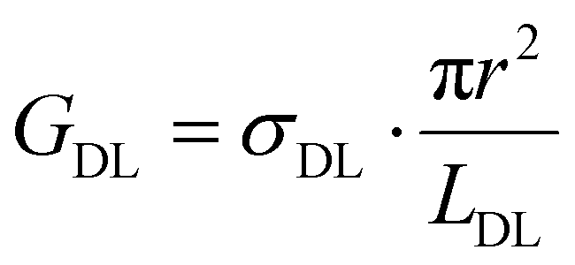
The double layer conductance G_DL is related to the charge distribution and interaction between the surface of the nanopore and the electrolyte solution. σ_DL is the conductivity of the double layer, typically dependent on surface charge density, ion type, and solution conditions; L_DL is the effective thickness of the double layer, which is around 0.77 nm for a 1 M LiCl solution. It is calculated as follows:

After calculating both contributions, we found that the bulk conductance is significantly larger than the double-layer conductance. The bulk conductance, calculated as 2.6 × 10⁻⁸ S, is the dominant factor in determining the total conductance of the nanopore. While the double-layer conductance does play a role, its contribution is comparatively smaller, with a calculated value of 4.16 × 10⁻¹¹ S.

By considering both factors in our model, we gained a more complete picture of the overall conductance, confirming that the primary influence comes from the bulk ionic conductivity, while the effect of the double layer is minimal, particularly at high salt concentrations such as 1 M LiCl. This comprehensive approach ensures that the model used in our analysis is more robust and accurate in predicting the total conductance of the system.

Signal file acquisition suggestions

The resolution of the signal files has a certain impact on data extraction performance, and this limitation primarily arises from the combination of sampling rate and filter settings. While these settings optimize noise suppression and signal clarity, they limit the resolution required for ultra-fast event detection. The following strategies can be employed to improve temporal resolution and capture faster translocation events:

Appropriate voltage. By reducing the voltage applied across the nanopore, the speed of molecules passing through the pore can be slowed, thereby increasing the duration of the events. This allows for more complete signal features to be captured at higher temporal resolution.

Nanopore modification. Modifying the nanopore surface can further adjust the interaction between molecules and the nanopore, controlling the speed at which molecules pass through. Appropriate modifications help slow down the molecules’ flow, enabling translocation events to be captured and analyzed at higher temporal resolution.

Optimizing acquisition parameters. By adjusting filter cutoff frequencies and increasing the sampling rate, we can improve the temporal resolution while maintaining an acceptable signal-to-noise ratio. This will enhance the detection of fast translocation events.

These optimization strategies can improve the detection of fast translocation events, providing more complete and reliable raw data for the signal extraction algorithm, thereby enhancing the accuracy and effectiveness of the algorithm.

Program coding

Qt designer platform was used to design the visual interface of the software, Python was used to develop the back-end function of the software, and the key libraries used by the software included pyabf, pyqt5, and matplotlib.

Results and discussion

Signal model and program algorithm

In this paper, the many aspects of nanopore data analysis have been described in our nanopore signal model. During the recognition of the signal, the event detection thresholds (start and end thresholds determine the start and end points of the event, respectively) are determined based on the magnitude of the change in the current pulse with respect to the baseline. Thus, the accuracy of the value of the baseline determines the outcome of the nanopore signal recognition. To identify the translocation event, the signal recording is segmented in slidable windows, and the local mean and local variance for each window are computed as a means of dynamically assessing the baseline drift and determining the event detection threshold. Thus, a nonlinear threshold curve is generated according to the statistical characteristics of the signal in the window, which can flexibly adapt to the dynamic changes of the signal, especially in the case of large fluctuations of baseline current and mass dense pulse signals. Consequently, the baseline and threshold can be dynamically corrected in real time to resist the disturbance effect to improve the accuracy of event detection. The procedure is split into a series of successive stages, with each stage utilizing parameters determined in the previous stage, as shown in Fig. 1.

Fig. 1 Flow chart of the dynamic correction method.

The Dynamic correction method comprises the following steps.

Step 1: Window Initialization. First, three concepts are clarified. Window size (W) refers to the number of sample points considered at one time when processing the signal. Sampling frequency (f) refers to the number of sample points collected per second in Hz, and the sampling frequency determines the time resolution of the signals. Time (t) is the actual time covered by the window, which can be calculated from the window size and sampling frequency. The mathematical relationship between the three parameters is expressed as:

The next steps are to set the appropriate window size (W), step size (S) and buffer size (B), and scan the entire signal file by sliding the window. During each movement of batch windows, the data within the window and (the contextual components in the front and rear areas) the buffer before and after it are further adjusted and processed based on cascade feedback. Setting the signal as x and the length as N, a sliding window function f(k) can then be defined with k denoting the index of the window and i denoting the signal point index as follows.

f(k) = {x[i]|(k − 1)S ≤ i < kS + W}, for k = 1, 2,…, N/S (2)

For each index k, the sliding window function f(k) returns a collection of consecutive data points of number W that are signals x from position (k − 1)S to kS + V − 1. This formula assumes that the step size S is less than or equal to the window size W, ensuring the overlap between the windows. If the step size S is greater than the window size W, there will be no overlap between the testing windows. This formula also assumes that the signal length N is an integer multiple of the step size S, which ensures that the last data point of the signal is exactly at the end of a window. If the signal length N is not an integer multiple of the step size S, then the last window may contain fewer data points, or the signal may need to be filled or truncated accordingly. The window is then scrolled through the entire signal according to the selected step size. After each sweep, the working data within the window and the connected data near the windows are ready for the next processing step.

Step 2: Preliminary Threshold Initialization. The mean variance within the window is the primary part of calculating the preliminary threshold. Here a first-order digital low-pass filter is used to calculate the local mean and variance at each point of the original signal with the following formulae.

ml(i) = α × ml(i − 1) + (1 − α)S_raw(i), i = 1, 2,… (4)

vl(i) = α × vl(i − 1) + (1 − α)[S_raw(i) − ml(i)]², i = 1, 2,… (6)

Here, S_raw(i) is the i-th point of the original signal. ml(i) and vl(i) are the local mean and local variance of the original signal at the i-th point, respectively. T_us(i) and T_ds(i) are the global mean and the global variance of the original signal, respectively, and α represents the coefficients of the filter. T_us(i) and T_ds(i) represent the start thresholds for the amplitude increase and decrease, respectively. The parameter β_s is used to calculate a preliminary threshold for event detection by setting a distance between a signal point and the local mean (baseline level), where the value of this distance is s times the local standard deviation, and signal data with current fluctuations greater than this distance are filtered. With greater values of s, the preliminary threshold for event detection will be higher and the algorithm will be less sensitive to the event.

Step 3: Data Filtering. Some points that are significantly below the current threshold are filtered out. The filtering action of signals will traverse the entire window, and the new thresholds derived from step 2 are constantly set depending on the correction process. If the sudden change of the current data is more than the specified threshold, an event is considered to be identified and the starting points are recorded in a list.

Step 4: Event Detection Threshold Correction. The Dynamic correction method (Fig. 2a) calculates the mean and variance within a localized window, and obtains a baseline (red dashed line) and an event detection threshold (blue dashed line). A user-configurable yellow pane is displayed within the signal file. Upon the detection of a recordable event, the window initiates a baseline correction. This involves replacing the mean and variance values within the baseline calculation for the specified area with the mean and variance values at a number of points located prior to and subsequent to the event's start and end points, respectively. The number of points included in this replacement is also adjustable. This dynamic adjustment process brings the event detection thresholds of the pane-formatted file closer to the baseline, thereby ensuring greater accuracy in the values of each feature of each recorded event. Concurrently, this process is tantamount to circumventing the interference occasioned by the fluctuating current of the event in question with each instance of its documentation, thus ensuring that the event detection threshold remains unimpaired. For comparison, the baseline scanning method is illustrated in Fig. 2(b). As events are detected, the cumulative changes in the mean and variance of the entire window can shift the event detection threshold, which may affect the signal recognition accuracy. This shift can lead to small signals being masked or the characteristics of the detected signals becoming inaccurate. In contrast, the Dynamic Correction Method dynamically adjusts the threshold in real time, mitigating the impact of such shifts. By localizing the threshold change curve, this method better fits the local signal characteristics, enhancing the detection sensitivity. Additionally, it allows for more precise extraction of event features, such as duration and amplitude, improving the accuracy and reliability of signal detection, especially in complex or low signal-to-noise ratio environments.

Fig. 2 Identification of transition events by different methods. (a) Dynamic correction method; (b) baseline scanning method.

Step 5: Event identification. As above, the end threshold will be determined based on the local mean and local variance to detect the events in the current traces. Meanwhile, the data between the start and the end of the events are checked back and forth according to the upward and downward threshold to reach its optimal results. The formula for the event end threshold is shown as below.

Here, T_ud(i) and T_de(i) represent the thresholds with upward and downward amplitude for independent event recognition, respectively, and β_e is a parameter used to compute the end threshold. It controls the distance between the end threshold and the local mean, which is e times the local standard deviation. With greater values of e, there is a lower end threshold, and the algorithm becomes more stringent in determining the end of the event. By adjusting the values of s and e, it is possible to regulate the sensitivity of the algorithm to events, as well as its requirement for the duration of events. The application of larger values of s will result in a reduction of the number of events that are identified, although this may result in the omission of some true events. Conversely, the application of larger values of e will increase the duration of events. However, this may result in the misclassification of certain noise as part of the event. In practice, the values of s and e should be set according to the specific characteristics of the signal and the requirements of the application in order to achieve the optimal results in event detection.

Step 6: Screening of Events. The detected events are subjected to screening according to preset conditions with the objective of eliminating possible false positives.

Step 7: Feature extraction. Save the current event information and calculate its features. Output the relevant information of the filtered events into the result array.

Step 8: Slide the window to subsequent data processing. Perform the detection of the translocation event in the next window.

Event characterization for nanopore sensing for polymerase

In order to assess the efficacy of the Dynamic correction method, we conducted experiments using polymerase as the target for detection. The concentration of polymerase used was 50 μM, and the experiments were performed on solid-state nanopores with a pore size of 25 nm and an applied voltage of 400 mV. The nanopore blockage current signal of these experiments are presented in Fig. 3a.

Fig. 3 Enhancement of data accuracy after applying the dynamic correction method and baseline scanning method. (a) Nanopore blockage current signal graph of polymerase. (b) Duration distribution of the nanopore signal using the baseline scanning method. (c) Blockage current distribution of the nanopore signal using the baseline scanning method. (d) Duration distribution of the nanopore signal using the dynamic correction method. (e) Blockage current distribution of the nanopore signal using the dynamic correction method. (f) Scatter plot of the signals from the two methods.

To evaluate the improvement brought about by our algorithm, we analyzed the signal distributions by applying the Dynamic correction method (counts: 865) and Baseline scanning method (counts: 841). The signal amplitude and width distributions were fitted using a Gaussian function model, and the fitted curves are depicted as dashed lines in Fig. 3. The goodness of fit was assessed using the R-square values, which were found to be 0.827, 0.877, 0.905, and 0.988 for Fig. 3b–e, respectively. Our analysis revealed that the time of the signals in relation to the bar graph of the blockage current of the half-peak width became narrower after applying the improved algorithm. This indicates that the data became more concentrated. Additionally, the fitted peaks in Fig. 3b–e were determined to be 0.135 ms, 0.161 ms, 8991.4 pA, and 9003.2 pA, respectively. The consistency of these peaks suggests that our algorithm optimizes the identification process, while maintaining the accuracy of the data. Fig. 3f compares the signal data obtained using the Dynamic correction method (red) with the data obtained using the Baseline scanning method (black). The data points derived from our algorithm are concentrated in the center region, which is crucial for the classification of solid-state nanopore signals. This observation suggests that we can obtain various features of the sample using a smaller sample size. Overall, our findings demonstrate the effectiveness of our algorithm in improving the analysis of solid-state nanopore signals.

Dynamic correction method for the classification of signals from gold nanoparticles

Due to the limitations of the micro- and nanofabrication process, the baseline current of solid-state nanopores often fluctuates to a large extent, which can affect the accuracy of signal recognition. At the same time, the extent of such fluctuations is also related to the substance to be measured. For example, proteins are more likely to cause baseline fluctuations compared to DNA. With increasing spatial volume of the substance, it is more likely for a collision process to be formed during the pore entry process, thus causing baseline fluctuations. The more rigid metal nanoparticles are more likely to cause irregular oscillations of the nanopore baseline currents because they tend to form clusters in the salt solution. As shown in Fig. 4a, we detected two kinds of gold nanoparticles with particle sizes of 10 nm versus 15 nm (both with a concentration of 20 nM) using a solid nanopore with a pore size of 20 nm, and the mixed samples of metal particles made the nanopore baseline fluctuation very unstable. In this study, the term “ionic current fluctuations” refers to variations in the ionic current signal caused by multiple factors. These fluctuations can be classified into two types: slow fluctuations and fast fluctuations. Slow fluctuations primarily arise from electrochemical reactions occurring near the nanopore orifice, leading to gradual changes in the baseline current. In contrast, fast fluctuations are typically caused by the dynamic oscillatory motions of particles at the nanopore orifice, resulting in rapid and short-lived changes in the ionic current. Notably, the nanopore chips used in this study were fabricated using a dielectric breakdown method, which differs from traditional approaches involving high-energy electron or ion beam drilling. This method offers advantages, including low cost and rapid pore formation. The process involves the initial creation of a small pore via breakdown and then gradually enlarging it, resulting in a more loosely configured pore structure. This structural characteristic makes ionic current fluctuations, particularly those caused by particle motion, more likely to occur. Fig. 4b shows the signal counting using the Baseline scanning method to count the signals. The number of signals for the two kinds of particles (10 nm and 15 nm) is 128 (red) and 405 (green), respectively. Fig. 4c shows the signal counting graph after using the Dynamic correction method. The number of signals for the two kinds of particles is elevated to 418 (red) and 691 (green), respectively. It can be clearly seen from the graphs that with the increase in the number of signals recognized, there is not a significant change in aggregation and distribution of signals. In particular, it should be noted that the concentration of the 10 nm and 15 nm gold nanoparticles is 20 nM. Theoretically, there is not much difference in the capture probability of the two sizes, but the capture frequency ratio under the Baseline scanning method is only 31% (128/405). This means that baseline fluctuations and signal complexity will affect the acquisition of small signals. However, when we use the Dynamic correction method to process the same batch of files, the capture frequency ratio increases to 60% (418/691), which reflects the improvement of the threshold adjustment for complex sample signal acquisition, especially when the baseline fluctuation is obvious.

Fig. 4 (a) Signal recognition of nanopore signals under a fluctuating baseline (the test sample is a mixture of 10 nm and 15 nm gold nanoparticles). (b) Distribution of nanopore signals detected by the baseline scanning method. (c) Distribution of nanopore signals detected by the dynamic correction method.

We have counted the signal distributions obtained by the Baseline scanning method and Dynamic correction method, and the results are shown in Fig. 5, where panels (a) and (b) show the distribution of the blocking current versus pore time for the 10 nm gold nanoparticles, and panels (c) and (d) show the distribution of the blocking current versus pore time for the 15 nm gold nanoparticles. The most significant difference is 0.041 ms in Fig. 5b (1.028 ms and 1.069 ms for the Baseline scanning method and Dynamic correction method, respectively), while the difference in the blocking current is much smaller, with 86.45 pA and 53.70 pA for the 10 nm and 15 nm gold nanoparticles, respectively. This demonstrates that the Dynamic correction method can significantly improve the signal recognition rate while maintaining the signal characteristics, especially for smaller current signals that are missed due to baseline fluctuations.

Fig. 5 Signal distributions obtained by the baseline scanning method and dynamic correction method. Panels (a) and (b) correspond to current versus transit time for the 10 nm gold nanoparticles, and panels (c) and (d) correspond to current versus transit time for the 15 nm gold nanoparticles.

Conclusion

Overall, we developed a software program to perform baseline correction in real time using the Dynamic correction method, overcoming the interference of baseline fluctuations of solid-state nanopores and solving the difficult problem of detecting small and medium signals in signal-dense regions. This improves the acquisition rate and accuracy of nanopore signals. The data obtained from biomolecules, including enzymes and nanoparticles, after the application of our dynamic correction method to solid-state nanopores demonstrates effective signal recognition. This study encompasses a range of topics related to biochemical experiments, signal processing, and data analysis. Furthermore, it offers valuable insights into solid-state nanopore signal research by employing the technique of dynamic correction of event detection thresholds to address the current challenges in solid-state nanopore signal analysis.

Author contributions

GX conceived and designed the study, developed the program, conducted the experiments, and drafted the original manuscript. JS was responsible for module construction. JM performed data analysis. LW revised the manuscript. JT supervised the study, managed the project administration, and finalized the manuscript.

Data availability

The clients for Windows, Linux, and MacOS operation systems are available and can be downloaded from https://github.com/eventdetector/Event-Detector.

The source code can be downloaded from https://github.com/eventdetector/Event-Detector-Code.

All data included in this article are available from the authors upon request.

Conflicts of interest

The authors declare no conflict of interest.

Acknowledgements

This work was supported by the Key Research and Development Project of Jiangsu Province (BE2022804) and the Fundamental Research Funds for the Central Universities (2242023K5005).

References

1. A. J. Storm, C. Storm, J. Chen, H. Zandbergen, J.-F. Joanny and C. Dekker, Fast DNA Translocation through a Solid-State Nanopore, Nano Lett., 2005, 5(7), 1193–1197.
2. C. Dekker, Solid-state nanopores, Nat. Nanotechnol., 2007, 2(4), 209–215.
3. D. Branton, D. W. Deamer, A. Marziali, H. Bayley, S. A. Benner, T. Butler, M. Ventra, S. Garaj, A. Hibbs and X. Huang, The potential and challenges of nanopore sequencing, Nat. Biotechnol., 2008, 26(10), 1146–1153.
4. S. Howorka and Z. Siwy, Nanopore, analytics: sensing of single molecules, Chem. Soc. Rev., 2009, 38(8), 2360–2384.
5. C. Cao and Y.-T. Long, Biological Nanopores: Confined Spaces for Electrochemical Single-Molecule Analysis, Acc. Chem. Res., 2018, 51(2), 331–341.
6. G. M. Cherf, K. R. Lieberman, H. Rashid, C. E. Lam and M. Akeson, Automated Forward and Reverse Ratcheting of DNA in a Nanopore at Five Angstrom Precision, Nat. Biotechnol., 2012, 30(4), 344–348.
7. F. J. Rang, W. P. Kloosterman and D. R. Jeroen, From squiggle to basepair: computational approaches for improving nanopore sequencing read accuracy, Genome Biol., 2018, 19(1), 90.
8. B. Kyle, K. Harold and T.-C. Vincent, Automated Fabrication of 2 nm Solid-State Nanopores for Nucleic Acid Analysis, Small, 2014, 10(10), 2077–2086.
9. R. S. S. De Zoysa, D. A. Jayawardhana, Q. Zhao, D. Wang, D. W. Armstrong and X. Guan, Slowing DNA translocation through nanopores using a solution containing organic salts, J. Phys. Chem. B, 2009, 113(40), 13332–13336.
10. Y. Rozevsky, T. Gilboa, X. F. V. Kooten, D. Kobelt and A. Meller, Quantification of mRNA Expression Using Single-Molecule Nanopore Sensing, ACS Nano, 2020, 14(10), 13964–13974.
11. C. Diego, G. Nicoletta, K. Agne, C. Pierre-Eugene, C. Benoit, J. Jean-Marc and B. Sebastien, Unexpected Hard Protein Behavior of BSA on Gold Nanoparticle Caused by Resveratrol, Langmuir, 2018, 34(30), 8866–8874.
12. A. Arima, I. H. Harlisa, T. Yoshida, M. Tsutsui, M. Tanaka, K. Yokota, W. Tonomura, J. Yasuda, M. Taniguchi and T. Washio, Identifying Single Viruses Using Biorecognition Solid-State Nanopores, J. Am. Chem. Soc., 2018, 140(48), 16834–16841.
13. H. Chae, D. K. Kwak, M. K. Lee, S. W. Chi and K. B. Kim, Solid-state nanopore analysis on conformation change of p53TAD–MDM2 fusion protein induced by protein–protein interaction, Nanoscale, 2018, 10(36), 17227–17235.
14. S. W. Kowalczyk, A. R. Hall and C. Dekker, Detection of Local Protein Structures along DNA Using Solid-State Nanopores, Nano Lett., 2010, 10(1), 324–328.
15. D. Coglitore, P. E. Coulon, J. M. Janot and S. Balme, Revealing the Nanoparticle-Protein Corona with a Solid-State Nanopore, Materials, 2019, 12(21), ma12213524.
16. M. Raveendran, A. R. Leach, T. Hopes, J. L. Aspden and P. Actis, Ribosome Fingerprinting with a Solid-State Nanopore, ACS Sens., 2020, 5(11), 3533–3539.
17. D. Branton, D. W. Deamer, A. Marziali, H. Bayley, S. A. Benner, T. Butler, M. Di Ventra, S. Garaj, A. Hibbs and X. Huang, The potential and challenges of nanopore sequencing, Nat. Biotechnol., 2008, 26(10), 1146–1153.
18. E. C. Yusko, B. R. Bruhn, O. M. Eggenberger, J. Houghtaling, R. C. Rollings, N. C. Walsh, S. Nandivada, M. Pindrus, A. R. Hall and D. Sept, Real-time shape approximation and fingerprinting of single proteins using a nanopore, Nat. Nanotechnol., 2017, 12(4), 360–367.
19. W. Yang, L. Restrepo-Pérez, M. Bengtson, S. J. Heerema, A. Birnie, J. V. D. Torre and C. Dekker, Detection of CRISPR-dCas9 on DNA with Solid-State Nanopores, Nano Lett., 2018, 18(10), 6469–6474.
20. M. Wang, A. Fu, B. Hu, Y. Tong and T. Liu, Virus Detection: Nanopore Targeted Sequencing for the Accurate and Comprehensive Detection of SARS-CoV- and Other Respiratory Viruses, Small, 2020, 16(32), 2002169.
21. H. Tang, H. Wang, C. Yang, D. Zhao and Y. Li, A novel strategy for nanopore-based selective detection of single carcinoembryonic antigen (CEA) molecules, Anal. Chem., 2020, 92, 3042–3049.
22. V. Tabard-Cossa, M. Wiggin, D. Trivedi, N. N. Jetha and A. Marziali, Single-Molecule Bonds Characterized by Solid-State Nanopore Force Spectroscopy, ACS Nano, 2009, 3(10), 3009–3014.
23. Z. Sun, X. Liu, W. Liu, J. Li, J. Yang, F. Qiao, J. Ma, J. Sha, J. Li and L. Q. Xu, AutoNanopore: An Automated Adaptive and Robust Method to Locate Translocation Events in Solid-State Nanopore Current Traces, ACS Omega, 2022, 7(42), 37103–37111.
24. Y. M. N. D. Y. Bandara, S. Dutt, B. I. Karawdeniya, J. Saharia, P. Kluth and A. Tricoli, A Robust Parallel Computing Data Extraction Framework forNanopore Experiments, Small Methods, 2024, 8(12), 240045.
25. Y. M. N. D. Y. Bandara, J. Saharia, B. I. Karawdeniya, P. Kluth and M. J. Kim, Nanopore Data Analysis: Baseline Construction and Abrupt Change-Based Multilevel Fitting, Anal. Chem., 2021, 93(34), 11710–11718.
26. C. Raillon, P. Granjon, M. Graf, L. J. Steinbock and A. Radenovic, Fast and automatic processing of multi-level events in nanopore translocation experiments, Nanoscale, 2012, 4(16), 4916–4924.
27. C. Plesa and C. Dekker, Data analysis methods for solid-state nanopores, Nanotechnology, 2015, 26(8), 084003.
28. J. H. Forstater, K. Briggs, J. Robertson, J. Ettedgui, O. Marie-Rose, C. Vaz, J. J. Kasianowicz, V. Tabard-Cossa and A. Balijepalli, MOSAIC: A Modular Single-Molecule Analysis Interface for Decoding Multistate Nanopore Data, Anal. Chem., 2017, 88(23), 11900–11907.
29. J. Tu, H. Meng, L. Wu, G. Xi, J. Fu and Z. Lu, EasyNanopore: A Ready-to-Use Processing Software for Translocation Events in Nanopore Translocation Experiments, Langmuir, 2021, 37(33), 10177–10182.
30. J. Zhang, X. Liu, Y. L. Ying, Z. Gu, F. N. Meng and Y. T. Long, High-bandwidth nanopore data analysis by using a modified hidden Markov model, Nanoscale, 2017, 9(10), 3458–3465.
31. M. Tsutsui, T. Takaai, K. Yokota, T. Kawai and T. Washio, Deep Learning-Enhanced Nanopore Sensing of Single-Nanoparticle Translocation Dynamics, Small Methods, 2021, 5(7), e2100191.
32. Z. X. Wei, Y. L. Ying, M. Y. Li, J. Yang and Y. T. Long, Learning shapelets for improving the single-molecule nanopore sensing, Anal. Chem., 2019, 91(15), 10033–10039.
33. D. Dematties, C. Wen, M. D. Pérez, D. Zhou and S. L. Zhang, Deep learning of nanopore sensing signals using a bi-path network, ACS Nano, 2021, 15(9), 14419–14429.
34. D. Dematties, C. Wen and S. L. Zhang, A Generalized Transformer-Based Pulse Detection Algorithm, ACS Sens., 2022, 7(9), 2710–2720.
35. K. Misiunas, N. Ermann and U F. Keyser, QuipuNet: Convolutional Neural Network for Single-Molecule Nanopore Sensing, Nano Lett., 2018, 18(6), 4040–4045.

---