
 Open Access Article
 This Open Access Article is licensed under a
 Creative Commons Attribution 3.0 Unported Licence
Faceted wrinkling by contracting a curved boundary†
Anshuman S.
Pal
 a,
Luka
Pocivavsek
b and
Thomas A.
Witten
*a
a,
Luka
Pocivavsek
b and
Thomas A.
Witten
*a
aJames Franck Institute and Dept. of Physics, University of Chicago, IL, USA. E-mail: t-witten@uchicago.edu
bDept. of Surgery, Pritzker School of Medicine, University of Chicago, Chicago, IL, USA
First published on 5th April 2024
Abstract
Single-mode deformations of two-dimensional materials, such as the Miura-ori zig-zag fold, are important to the design of deployable structures because of their robustness; these usually require careful pre-patterning of the material. Here we show that inward contraction of a curved boundary produces a fine wrinkle pattern with a novel structure that suggests similar single-mode characteristics, but with minimal pre-patterning. Using finite-element representation of the contraction of a thin circular annular sheet, we show that these sheets wrinkle into a structure well approximated by an isometric structure composed of conical sectors and flat, triangular facets. Isometry favours the restriction of such deformations to a robust low-bending energy channel that avoids stretching. This class of buckling offers a novel way to manipulate sheet morphology via boundary forces.
The flourishing field of extreme mechanics4–7 seeks ways in which large, spontaneous material deformations yield robust, reproducible structures and motions. Many of these structures exploit the selective deformations shown by thin sheets, which bend or fold easily but resist internal stretching strongly.8–19 The large resistance to stretching creates strong, non-local constraints that restrict the sheet to selected modes of deformation. A classic example is the Miura-ori folding pattern.1,20,21 This periodic pattern enables one to contract a spread-out flat sheet of paper into a compactly folded state with one single mode of deformation dictated by the pattern (see Fig. 1a). Here we report similar robust deformation of a flat sheet without the position-dependent processing needed for an origami fold. Instead, we specify an initial annular shape and a simple mode of edge deformation: contracting the inner boundary radially. The result is a strongly reproducible three-dimensional pattern of high-amplitude wrinkles. We attribute the reproducibility to a qualitative feature of the simulated, finite-element simulation—each wrinkle approaches an isometric shape, with no stretching. This unstretched morphology is made possible by a distinct pattern of flat, triangular facets alternating with smoothly-curving conical segments.
 | ||
| Fig. 1 Geometry-controlled robust radial wrinkling. (a) Miura-ori patterns guide a flat sheet to contract into a folded state with a single, continuous motion (adapted from ref. 1). (b) Smooth radial (i.e., Lamé) wrinkling in an annulus under both inner and outer tension, indicated by arrows (adapted from ref. 2). In this paper, we study Miura-ori like robust deformation of an annulus in a radial Lamé setting. This deformation can be generated in multiple ways. (c) Finite-element calculated shape under uniform radial contraction of the inner boundary, described in Methods (inset shows detail of emergent zigzag inner boundary). (d) Circular-cone-triangle geometric construction defined in Section 2, with triangles shown in blue and cones in red. (e) Ruff collar garment (reproduced from ref. 3) made by manually pleating the inner boundary of an annular piece of cloth. | ||
We consider a minimal form of radial contraction that we call “inner Lamé” contraction. We displace the inner boundary of the annulus with no further constraints. Our interest in this geometry arose from experiments on the curling of edge-connected polymeric sheets with unequal solvent swelling. Ref. 22 shows the result for two half sheets with different swelling separated by a straight boundary. We simulated the radial analogue of this situation, where the straight boundary was replaced by a circular boundary separating an inner region with little swelling from an outer one with more swelling. The swelling resulted in fine radial wrinkling like that shown in Fig. 1. The present simplified system was developed to understand this wrinkling.
As shown in Fig. 1c, the inner Lamé contraction produces fine wrinkling like the conventional Lamé contraction of Fig. 1b. However the two wrinkled states are radically different. The conventional Lamé wrinkle wavelength is explained in terms of the applied tension.2 However, in the inner Lamé, the exterior tension of the Lamé state is absent, and so the established mechanism for the wrinkle wavelength cannot apply. Indeed, our wrinkling contrasts with most wrinkled systems, where the bending energy favoring longer wavelengths is countered by the energy associated with some external forcing.9,23 The wrinkle wavelength then depends explicitly on the strength of this forcing. The inner Lamé system has no such strength parameter. Instead, the deformation is defined in terms of the geometric displacement of the inner edge only.
Even among geometrically-defined forms of wrinkling, the inner-Lamé geometry is anomalous. A priori, it doesn't conform to typical one-dimensional buckling treatable as an Euler elastica system.24 Other forms in which the constraint is applied at one boundary14,25 do not give a well-defined wave number as we find.
Furthermore, we note that the forms of wrinkling mentioned above are explained as equilibrium ground-states of the system. In our system the wrinkles emerge from a quasistatic deformation. That is, the inner displacement is applied gradually, and the configuration is allowed to relax at every stage. This procedure corresponds to how one would perform the deformation experimentally. In this limit, the system follows a given energy minimum as the deformation is imposed. It need not be an energy ground state.
In this paper, we address the structure of the individual wrinkles resulting from this unusual mode of deformation.‡ We show that a strain-free isometric shape quantitatively accounts for observed features of our simulated shape, notably the elastic energy shown in Fig. 5. This energy contrasts strongly with the much higher energy expected with a simple sinusoidal wrinkling pattern (Section 3.3). Moreover, the simulated deformation matches an explicitly isometric deformation of the original annulus into a cone-triangle pattern. We describe the robustness of the structure using a variety of initial and boundary conditions for the contracted inner boundary. We argue that the observed robustness of the cone-triangle structure is a natural consequence of its isometric property. We note how the cone-triangle structure can be induced via different paths, as illustrated in Fig. 1c–e, and discuss generalisations to a broader range of structures. Using the findings of this paper, we address the question of wavelength determination in a separate work.26
Sections 1 and 2 define the inner Lamé deformation that we simulate, and the isometric model shape used for comparison. In Section 3, we show that the shape and energy of the simulated sheet are consistent with the model. Section 4 addresses our assumptions and discusses the value of such deformations for generating spontaneous structures. Finally, Section 5 gives an account of our numerical methods.
1 Inner Lamé deformation
Given the circular annulus of Fig. 2a, we define the inner Lamé deformation as the equilibrium shape induced by drawing the inner boundary inward by a distance Δ, so that it is forced to live on a cylinder whose radius is reduced by Δ.§ We define the initial inner radius as our unit of length. The pull distance Δ thus acts as the sole loading parameter in the system. The system can thus be conveniently defined using only three geometric parameters: thickness t, the width w, and displacement ‘loading’ Δ. The internal forces determining the shape arise from the bending modulus B and the in-plane stretching modulus Y. Here, we seek the asymptotic behaviour of our annulus in the thin limit: t ≪ w; t ≪ 1. | ||
| Fig. 2 (a) Sketch of the inner Lamé deformation of a horizontal annulus. (Top) Top view showing the undeformed annulus, of inner radius 1 and width w. (Bottom) Vertical cross-section of the deformed annulus through a line where the vertical displacement of the wrinkle is maximal. The undeformed state is shown in light shading; the dark lines are a section of the deformed annulus, contracted horizontally by a distance Δ. These lines are also displaced upward and tilted downward. (b) Sketch of the circular-cone-triangle construction in its initial, flat state. Here we choose wavenumber m = 6, hence it has 12 triangles (shown in colour). The mid-line and height w of one triangle are indicated. The sectors bridging the triangles are shown in white; S is its outermost arc length. When the bases of the triangles are moved inward, they must tilt to retain their shape and connectivity. The bridging sectors are squeezed laterally to form cones. A typical deformed example is shown in Fig. 1c. (c) Top view of a narrow sector of the sheet, with detail of an area element at the outer edge of Lamé sheet showing radial (horizontal) and azimuthal (almost vertical) boundary forces. In the fully buckled (FT) regime,2 the azimuthal forces nearly vanish (as indicated by the upper and lower X's). In the the present “inner Lamé” system, the outer radial force also vanishes, indicated by the X at right. Thus, the inward radial force must also nearly vanish for force equilibrium. All elements to the left of the pictured one are subject to the same argument. Thus except for bending stresses, all radial stresses vanish. | ||
The conventional “FT” reasoning used to explain classical Lamé wrinkling2 suggests that fine wrinkling like that of Fig. 1. would require negligible radial stretching. In the FT regime, the wrinkling slopes grow to the order of unity, and the associated azimuthal stress becomes negligible compared to the pre-buckling stress. Only the bending azimuthal stress, owing to wrinkling, proportional to the bending modulus and the curvature, remains. The same is expected for our inner Lamé case: consider the radial stress in a narrow sector of the annulus (see Fig. 2c). Equilibrium requires that the net radial force on the sector be zero. In the unbuckled state, the inner tension driving the deformation is balanced by the net outward component of the azimuthal stresses on the sides of the sector. But in the FT regime, this stress is negligible, as argued above. In addition, there is no radial tension at the outer boundary. We conclude that the only forces to balance an inner tension are the weak bending stresses.
The absence of any deformation stress except for bending stress would imply that the sheet deforms only by bending in the thin limit. That is, it is isometric to the undeformed flat annulus. Such an isometric limit can be attained by wrinkles of diverging fineness.16,17 But if a limiting smooth shape is to exist, then it must obey the geometrical property of “developability”. That is, in view of Gauss's Theorema Egregium,27 there must be a straight generator line through each point of the surface that extends to the boundary without curving in space.28 In the next sections, we show that the contracted annulus is indeed consistent with a specific developable surface, suggested by the numerically determined shape.
2 A developable cone-triangle model
The faceted inner Lamé morphology of Fig. 1 suggests a further hypothesis: that the wrinkled morphology can be seen as a piecewise union of alternating flat triangles and curved conical sectors. We take this as the starting point for our geometric model. For a configuration with wavenumber m, we consider a flat configuration (see Fig. 2b) where the inner boundary is a 2m-sided polygon. Each segment of this boundary is the base of an isosceles triangle of height w. To complete the annulus, the apexes of adjacent triangles are joined with an arc. The constructed surface then consists of these triangles and the sectors joining them.One may readily specify an isometric deformation that allows the inner boundary of this structure to contract. We deform the initial surface by translating the base of each triangle inward toward the centre, specifying that the triangles remain rigid. In order to maintain their shape and connectivity, the triangles must tilt (i.e. rotate about their mid-lines) increasingly as they are drawn inward; adjacent triangles tilt in opposite directions. The sectors connecting two triangles must then also bend in order to remain connected to their triangles. A simple isometric choice for this deformation is to bend the flat sectors into circular conical arcs as the boundaries of each sector squeeze together. These arcs do not in general join smoothly with their adjacent triangles, as further discussed in Section 3.3.
3 Comparing simulated deformation with model
In this section, we test whether the isometric/developable cone-triangle construction is able to predict the quantitative features of our simulated inner Lamé deformation from Section 1. Our finite-element analysis (FEA) software Abaqus uses standard methods to represent the deformed equilibrium shape as the (cylindrical) inner boundary is gradually contracted inward. The inner boundary is allowed to buckle by moving along the cylinder (see Methods). For simplicity we restrict this motion to the axial direction, and allow no azimuthal motion of the boundary points. We describe the effect of this restriction in Section 4.3.4.In comparing this calculation to the cone-triangle construction, we must supply two free parameters: the boundary displacement Δ and the wavenumber m. Thus, we record the Δ and m of the finite-element deformation, and then construct the corresponding geometric solution with the same Δ and m. The first comparison we make is purely qualitative – we superpose the two solutions and observe how well they match up. Fig. 3 shows such a comparison, where we have rotated the geometric solution about the cylinder axis to obtain the best superposition. As the figure shows, one may align the two figures so that they overlay well over a significant part of the annulus, with matching zigzags at the inner boundary and matching waves at the outer boundary. Between the inner and outer boundaries, the surfaces match closely enough that the two surfaces alternately hide each other.
 | ||
| Fig. 3 Qualitative comparison between simulations and our cone-triangle model for a representative sample (w = 1.67, t = 1.33 × 10⁻³). (Left) Given w, Δ and the wavenumber m from the numerical solution, we construct a model cone-triangle solution (cones in red, triangles in blue) using the procedure described in Section 2. (Inset) Zoom-in of a single conical sector (in red) with the entire cone shown (in cream). S marks the length of the outermost arc (as in Fig. 2b) after deformation. For details of construction, see ESI.† (Right) For a qualitative comparison, we superpose the two solutions, with azimuthal rotation as the only degree of freedom. We find close agreement between them; with this top–down view, areas with colour indicate where the model solution is above the numerical solution, while those in grey indicate the opposite. In particular, the zoomed-in boxed portion shows close matching at both inner and outer boundaries. Specifically, the two inner boundaries show a regular zigzag shape of the same amplitude, which extends to qualitatively flat facets and terminates in a smoothly undulating outer boundary that also has similar amplitude in the two sheets. Zooming out to the whole annulus, we see that there is a ‘phase mismatch’ between the two solutions, with part of the solution in-phase (the boxed region) and part of it out-of-phase. This is due to the non-uniform size of the wrinkles in the numerical solution. | ||
The qualitative resemblance seen in the figure encourages a more quantitative comparison. In particular, we propose that for a given wave number m, the shape of the sheet approaches an isometric cone-triangle structure in the limit of zero thickness. Further, approximating each cone as a circular cone sector that connects its neighboring triangles gives a useful match to the shape and energy of the sheet.
Accurate comparison is hindered, however, by the variability of the simulated wrinkles. Though regular in general, the simulated wrinkle pattern is not strictly periodic on the annulus. To optimise the comparison, we perturb the initial flat state of the numerical sheet to promote periodicity. Specifically, we deform the initial state with a low-amplitude, smooth, periodic wrinkle with a wavelength similar to the original simulations.¶
3.1 Inextensibility and bending strains
We may roughly verify the anticipated isometry of the sheet as announced in the Introduction. To this end, we measure changes in lengths of the material circles at the inner (r = 1) and outer (r = 1 + w) boundaries.First, we consider radial inextensibility. Here, we use approximations appropriate for fine buckling and narrow wrinkles as in the far-from-threshold regime of ref. 2. A material circle at radius r in the annulus has fixed initial arc length L0(r) = 2πr. After the contraction, this circle deforms into a wavy line, whose horizontal projection is approximately circular under the observed fine buckling. The radius of this contracted circle is the original r plus some radial displacement er due to the inward contraction. The fractional change in the projected length Lxy is thus given by
| Lxy/L0 = 1 + er/r. | (1) |
 | ||
Fig. 4 Comparisons of geometric quantities between theory and simulations (using the explicitly periodic initial conditions described at the beginning of Section 3). (a) Testing radial inextensibility. The graph shows an average radial strain inferred from eqn (1), i.e. the small relative difference between the inward displacement at the outer boundary and that at the inner boundary, further discussed in Section 4.3.2. This example had w = 0.33, m = 25, and t = 2.67 × 10⁻⁴. (inset) Sketches of the wrinkle profile at the two boundaries, showing the definition of lengths L0 and Lxy, and slope angles αout and αin. The blue arrows indicate the compression direction. (b) Testing azimuthal inextensibility at the outer boundary. The magnitude of the residual azimuthal strain |εresidθθ| recorded slightly inside r = 1 + w, plotted logarithmically against the collective variable m2t2/(1 + w)2 at large Δ, for multiple values of m, t and w. The black line shows the linear fit:  . (c) Wrinkle slope angle vs. applied contraction . (c) Wrinkle slope angle vs. applied contraction ![[capital Delta, Greek, tilde]](https://www.rsc.org/images/entities/i_char_e10b.gif) ≡ Δ/r at the inner and outer boundaries (see Section 3.2). (top row) We separately test eqn (3) for αin (in red) and eqn (4) for αout (in black). The simulation data points are plotted alongside the model predictions. Simulated samples of differing width w and wavenumber m are coloured using the dimensionless cone splay parameter, ≡ Δ/r at the inner and outer boundaries (see Section 3.2). (top row) We separately test eqn (3) for αin (in red) and eqn (4) for αout (in black). The simulation data points are plotted alongside the model predictions. Simulated samples of differing width w and wavenumber m are coloured using the dimensionless cone splay parameter,  . The error bars are standard deviations from averaging over all the wrinkles. Markers: w = 0.33 (circles), w = 0.67 (squares), w = 1.0 (diamonds), w = 1.67 (triangles). (bottom row) Example wrinkle profiles for small and large η: (left) for η = 0.25 (w = 1.0, m = 25), and (right) for η = 1.8 (w = 0.33, m = 7). Colouring denotes height. . The error bars are standard deviations from averaging over all the wrinkles. Markers: w = 0.33 (circles), w = 0.67 (squares), w = 1.0 (diamonds), w = 1.67 (triangles). (bottom row) Example wrinkle profiles for small and large η: (left) for η = 0.25 (w = 1.0, m = 25), and (right) for η = 1.8 (w = 0.33, m = 7). Colouring denotes height. | ||
We may gauge azimuthal extensibility by measuring the full (not projected) change of arc length for the circle at radius r. Here we consider only the outer boundary region. As reported in Fig. 4b, there is a nonzero compression of these circles. This compression reflects the Elastica bending stress of pure bending mentioned in Section 1. Specifically, bending at a scale λ produces a residual bending stress, σresidθθ ∼ −B/λ2, where B is the bending modulus. Thus, from wrinkling of wavenumber m, we expect the outer boundary to have an azimuthal bending strain given by:
 | (2) |
Fig. 4a and b together provide suggestive evidence for radial and azimuthal inextensibility of the numerical solutions.
3.2 Evolution of wrinkle amplitude
We now compare specific features of the wrinkle shape to the predictions of the cone-triangle construction. In Fig. 4c, we consider the amplitude of the observed wrinkles. A dimensionless way of measuring the amplitude is by determining the average slope angle α of the wrinkles at the inner and outer boundaries. Though the cone-triangle construction can be implemented for a wide range of wavenumbers m for any given Δ and w, we considered only the narrow range of m that appeared spontaneously in the unperturbed numerics, where .26
.26
We define the average slope angle α to be the slope angle of the line joining the zero-crossing of the wrinkle with the adjacent maximum (illustrated in inset of Fig. 4a). For angle αin at the inner boundary, the figure explicitly relates αin to Lxy/L. For fine wrinkles, we may use eqn (1) to get:
cos![[thin space (1/6-em)]](https://www.rsc.org/images/entities/char_2009.gif) αin = 1 − Δ ≡ 1 − (1), αin = 1 − Δ ≡ 1 − (1), | (3) |
(r) ≡ Δ/r. At the outer edge, Lxy/L is likewise the ratio of the horizontal line to the arc length of the circular sector (see inset of Fig. 4a). For our circular cone model, it is related to the slope angle αout by| sin2αout/(2αout) = Lxy/L ≡ 1 − (1 + w). | (4) |
(r) for both inner (r = 1) and outer (r = 1 + w) boundaries. The upper red curve and data points compare αin. The agreement of the data points with the curve confirms that each triangle segment tilts to preserve its length as it is drawn towards the axis. The solid black curve gives the cone-triangle prediction of eqn (4) for αout. The data points on and beneath the curve represent annuli of different widths w and wavenumber m, coloured by their splay: η ≡ π(1 + w)/(mw). In general, our circular cone model is consistent with the prediction for narrowly-splayed wrinkles, but over-estimates the slopes for widely-splayed ones. The pictures below the graph show the annulus shape for different amounts of splay η. They suggest the source of the over-estimated slopes: for the widely splayed example with the greatest discrepancy, the boundary curve is significantly flatter than a circular arc. Thus the simplifying assumptions of our circular-cone construction are not satisfied in this widely-splayed regime.
3.3 Comparing energies
Perhaps the main significance of this isometric deformation is that its energy behaves so differently from that of a generically deformed sheet. It is different in two respects. Firstly, the energy depends only on the bending modulus B, and is independent of the stretching modulus Y for given bending modulus. Secondly, the energy in this limit is qualitatively smaller than for a generic wrinkling deformation with curvature and thickness comparable to our simulations. Below we verify that the energy of the contracted annulus has these distinctive features.The elastic energy is a sum of strain energy and bending energy:
| Uelastic = Ustrain + Ubend |
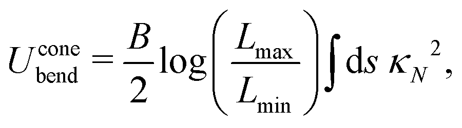 | (5) |
 | (6) |
 .
.
In eqn (6) only the quantity ρc(Δ) is not explicitly known. Our circular cone construction (see ESI†) permits us to get an expression for ρc(Δ) in terms of the outer slope angle αout:
 | (7) |
Our primary subject of interest, however, is the scaling of Umodelelastic with Δ for fixed m. Since  (see Fig. 4c), we expect the squared curvature and the bending energy to scale linearly with Δ: Umodelelastic ∼ 1/ρc2 ∼ Δ. We note that this linear form is the same as for the Elastica energy of a rod under weak Euler buckling,30 which is expected since each transverse arc of the cone undergoes Euler buckling with this same Δ dependence.
We may compare this isometric energy with that of conventional wrinkles17 whose height h(r,θ) has the separable form h = f(r)sin(mθ). As discussed in the ESI,† radial wrinkles of this form have substantial strain εc of order of εc ≃ Δ/m2, much larger than the bending strain of eqn (2), viz. ≃m2t2. Accordingly, for fixed Δ and m, the conventional strain εc and its associated elastic energy are much larger than their bending counterparts as t → 0. The ESI,† shows that εc is also large for the observed m values: εc ≈ 50εB.
In Fig. 5, we plot three energy curves for a typical sample. These curves compare the simulated energy for a typical example, Usimelastic(Δ) (lower curve), with two theoretical estimates: Umodelelastic(Δ) (upper curve; see eqn (6)) calculated from our cone-triangle model, and  (middle curve) calculated indirectly from the simulated solution through measurement of the mean squared curvature at the outer boundary:
 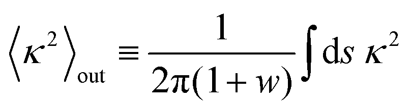 ,†† and by using eqn (5). The three curves are similar, differing by a roughly constant factor of order unity. Notably, the full simulated energy including any strain energy, is smaller than the model bending energies. This discrepancy is natural for the circular cone model, since this circular ansatz does not minimise the bending energy. The assumed uniform, circular curvature does not minimize the energy of the cone shape needed in order to bridge between the adjacent triangles. We expect that the system chooses a curvature profile κ(s) that minimizes this energy. Thus, as expected, the use of the measured κ(s) improves the agreement with the measured energy greatly. But a clear discrepancy remains.
 | ||
Fig. 5 Comparing elastic energies (see Section 3.3) for a representative sample (w = 1.0, m = 25, t = 6.67 × 10⁻⁴): Usimelastic(Δ) (lower curve); (see Methods) with Umodelelastic(Δ) (upper curve); (eqn (6)) and  (middle curve); (eqn (5)). All three curves show Elastica-like linear scaling (solid lines are fits), but the two theoretical curves overestimate the simulated energy by roughly 15% and 30% respectively. Other w and m values also generally over-estimated the energies, as discussed in Section 3.3. Energy units are defined in Methods. (inset) Annulus, indicating the region where energies were compared (in red), omitting the high-curvature regions near r = 1. (middle curve); (eqn (5)). All three curves show Elastica-like linear scaling (solid lines are fits), but the two theoretical curves overestimate the simulated energy by roughly 15% and 30% respectively. Other w and m values also generally over-estimated the energies, as discussed in Section 3.3. Energy units are defined in Methods. (inset) Annulus, indicating the region where energies were compared (in red), omitting the high-curvature regions near r = 1. | ||
We discuss the possible source of this discrepancy in ESI,† Section S7. It compares the simulated energy profile with that of a conical shape. The mismatch between the two profiles implies that the real surface does not have the straight director lines needed for a developably isometric surface. Such a mismatch requires strain energy. Accordingly, the mismatch should lessen with decreasing thickness. On the other hand this mismatch enables a reduction in bending energy below that of a cone. Thus the ESI† suggests how a small strain distortion can reduce the total energy below our isometric estimate, as the figure shows.
We conclude that the elastic energy of deformation for the wrinkles encountered in this study is strongly consistent with our claim of an isometric conical deformation. This minimal geometric picture gives a quantitative account of the structure and energy for a given wave number m. Residual discrepancies seem consistent with expected residual stretching effects. Furthermore, the explicit circular-cone-triangle construction gives a workable quantitative estimate of the full elastic energy. This approximation is least accurate when the splay parameter η is large.
4 Discussion
4.1 A developable wrinkling morphology
As shown above, the Lamé radial contraction system is qualitatively altered by removing the outer tension from that system. Specifically, the purely geometric definition of our deformation results in a faceted shape that is in clear contrast to prior force-based deformations.2,31,32 Our work demonstrates a strong resemblance between the observed shape and the exactly isometric cone-triangle shape defined above. For the numerically feasible thicknesses we report, the cone-triangle hypothesis allows us to reproduce structural and energetic features to good accuracy. Still, detailed analysis shows clear-cut departures from this shape that remain unexplained.Developable approximations such as the cone-triangle model appear to be a novel approach to describing periodic buckled structures. For the annular contraction deformation studied here, this developable picture seems entirely adequate as an initial quantitative account of the shape. This contrasts with other faceted shapes33,34 such as twisted ribbons,35 where a comparable understanding of the energy requires explicit consideration of non-developable geometry and non-bending energy. Our cone-triangle decomposition also provides an instructive example of a buckled shape in a radially symmetric system that does not have the conventional separable form – i.e. the buckling displacement is not a product of a radial factor and azimuthal factor.
The developability of the faceted wrinkling structure makes it fundamentally geometric, so that it can be created easily on a computer. This provides a way to programmatically construct smooth radially wrinkled patterns in materials using intrinsically flat components, much in the spirit of origami and other designed materials.7 In fact, a well-known real-world example of such programmed radial wrinkling is the Elizabethan ruff collar. One way of making a ruff is exactly using the inner Lamé boundary conditions: we take a cloth annulus, and manually make pleats in it such that the inner boundary of the annulus lives on a contracted radius. Fig. 1e and d show, respectively, a ruff collar and its reconstruction using our circular-cone-triangle model; the visual similarity between the two is striking. The conical outer solution seems to capture the ruff wrinkles, in particular their radial straightness and their shape at the outer boundary.
As noted above, accounting for the wrinkles of Fig. 1c is not equivalent to finding a ground-state configuration consistent with the imposed boundary condition. Our deformation was performed quasi-statically, and the wrinkles appeared continuously without abrupt jumps. Thus the system followed a single energy minimum as it deformed. This observed deformation may well have significantly higher energy than the ground state has.
4.2 Nature of the thin-sheet limit
The wrinkles investigated here closely approximate the isometric cone-triangle structure, in both shape and energy, as shown above. That is, many numerical examples with a broad range of thicknesses are well described by a model with no dependence on thickness. We take this as strong evidence that, for a given fine wrinkle number m ≫ max{1, 1/w}, the sheet approaches this isometric shape as thickness goes to zero. This leaves open the question of how the system selects this m, which clearly does depend on thickness. Given the present understanding of the energy and shape, the groundwork is laid to explain how this wrinkle number is selected. A separate paper by one of us26 addresses this question.4.3 Approximations and limitations
![[small script l]](https://www.rsc.org/images/entities/char_e146.gif) xy. The full displacement between inner and outer ends of the line is thus
xy. The full displacement between inner and outer ends of the line is thus  . For the data point in Fig. 4a at = 0.2, this effect adds a correction to the strain of +0.0002 to +0.0003, greatly reducing the reported value of strain. In addition, the material line is necessarily longer than displacement between its inner and outer ends. Further corrections come from localised strain effects near the inner boundary, as discussed in the next section.
Because of such corrections Fig. 4a shows only a rough consistency with the asymptotic isometry we claim here. For stronger evidence we rely on the energy measurements of Fig. 5.
One clear disagreement concerns the length of the inner boundary. In the simulation, the undeformed inner boundary is a circle. Under contraction, each tilted circular arc segment must stretch if it is to remain on the surface of a cylinder. Indeed, we observed such stretching along the inner boundary nodes. However, this stretching zone was confined to this first ring of nodes, with a much weaker stretching in the adjacent ring. In addition, we verified that the associated elastic energy was much smaller than that reported in Fig. 5.
The inexactness of the triangle construction at the inner surface makes it clear that the construction is not a realistic representation of a circular annulus contracted onto a cylinder for arbitrary wavenumber m. We demonstrated the isometric shape for only a limited range of geometries; both the displacement Δ and the width w were confined to moderate ranges. For these moderate conditions the system appears to choose wavelengths fine enough that the inaccuracies of the cone-triangle construction are not important. For more extreme ranges, we expect that the cone-triangle picture shown here will need modification and that the t → 0 limit will be more subtle. In particular, the locally stable isometric structure observed here may give way to macroscopic folding.23 Finding the conditions in which the cone-triangle wrinkles occur is a fruitful subject for future work.
4.4 Application
The deformation geometry treated here amounts to a strategy for avoiding the typical fate of deformed sheets. Such sheets adopt structures that require significant elastic energy beyond the needed bending energy. Often these structures produce uncontrolled disorder, e.g. as seen in a crumpled sheet. By contrast, the radial contraction used here guides the sheet into a locally low-energy channel resulting in only bending energy. This low-energy state is moreover attainable by continuous deformation from a flat reference state. Since these deformations lack the additional deformation costs of competing structures, they are intrinsically (locally) stable. They provide a general means to fold and compact a sheet continuously and reversibly with minimal external guidance. We note that the curved inner boundary appears important in stabilising this structure; straight boundaries with no radial contraction14 do not produce analogous regular wrinkling.These guiding channels should appear more generally than in the simple circular geometry studied here. The same principles control other inwardly curved boundaries, and other directions of contraction, e.g. onto a constraining cone instead of a cylinder.
4.5 Conclusion
While the emergence of developability in wrinkled systems has been studied intensively over the past decade, the simplicity and symmetry of the inner Lamé geometry makes it a particularly clean realisation of such a phenomenon. This faceted morphology is qualitatively different from previously known forms of two-dimensional wrinkling. Significantly, it creates sharply dictated, strongly distorted features with negligible stretching and without a separable radial/azimuthal shape. Moreover, it has many variants to be explored, with real world applications. Finally, this work sets the stage to explain the selection of the wavenumber m.265 Materials and methods
To investigate the wrinkling morphology of the inner Lamé system, we used the commercial finite-element (FE) solver Abaqus 2018 (SIMULIA, Dassault Systèmes). Using both implicit and explicit dynamic methods‡‡ in a quasi-static regime, we performed simulations of the inner Lamé system using its defining boundary conditions: radial displacement er(r = 1) = −Δ at the inner boundary mesh points, with the outer boundary nodes (at r = 1 + w) kept free. The maximum value of Δ applied was Δmax = 0.267.The simulation seeks the configuration that would be attained by adiabatically contracting the inner boundary (i.e., its nodes). Accordingly, it gradually decreases er from zero to −Δ as time t increases from 0 to tf. The value of tf is made sufficiently large that the kinetic energy is always a small fraction of the potential energy. Then the final configuration was not noticeably affected by further increase of tf, as detailed in the ESI.†
To account for the possibility of high strains, the sheet was initially modelled as a Neo-Hookean hyperelastic material with coefficients equivalent to the linear moduli: Young's modulus, E = 0.907125 MPa, and Poisson ratio, ν = 0.475 (cf.eqn (6)), corresponding to a rubber-like material. The associated bending stiffness B with thickness t is then given by  . To verify that results are independent of the material model, we also re-performed several simulations with a linear material model with these same moduli. Further details on our FEA methods are given in the ESI.†
To test the validity of our results over a range of parameters, we kept the inner radius fixed and varied the other two parameters – width w and thickness t – over the range of a decade. The width w of the annulus was varied between w = 0.33 (very narrow) to w = 1.67 (moderately wide) – a factor of almost 10. The thickness t was varied between t = 2.67 × 10⁻³ (thick) to t = 1.33 × 10⁻⁴ (very thin), a factor of 20. We performed consistency checks to ensure that the final morphology was independent of the choice of any simulation parameters. For data extraction, we used the software package Abaqus2Matlab.37
We used two principal deformation protocols to ensure that the wrinkles we observed were characteristic of the quasi-static limit. Our baseline protocol was done using explicit dynamics, in which the finite elements are accelerated with a constant damping factor. The other deformation protocol used an implicit scheme for integrating the forces, with the damping factor automatically selected by the software to favour quasi-static behaviour. In both cases, to avoid gross kinetic effects, we increased Δ from 0 to Δmax at a rate slow enough such that the kinetic energy of the system always remained  of the elastic energy. This is standard procedure for quasi-static analyses in finite-element simulations (see ESI,† for details).
The specifics of the wrinkling morphology depend on how the contracted boundary is constrained. For example, the clamped boundary studied by Mora and Boudaoud11 leads to a highly compressed boundary layer whose relation to the sheet is difficult to discern. The other extreme is to allow each point on the boundary circle to lie anywhere on the confining cylinder; such boundaries lead to wrinkling only in a transient regime, leading ultimately to collapse into a fold.23,38 Here we study an intermediate constraint in which points on the bounding circle may move only axially (i.e. vertically) on the bounding cylinder; azimuthal (θ) motion is not allowed. Doing so automatically prohibits folding (since this requires lateral motion), but without interfering with the wrinkling.
Author contributions
A. S. P. conceptualised the problem, performed simulations and measurements, and created the majority of the text and figures. L. P. was key in providing numerical support, and in critical readings of several drafts. T. A. W. supervised this work, formulated the cone-triangle model, and helped with conceptualisation, interpretation of data, writing and revising.Conflicts of interest
There are no conflicts to declare.Acknowledgements
The authors would like to thank Benny Davidovitch, Dominic Vella and Enrique Cerda for many insightful discussions, and Nhung Nguyen and George Papazafeiropoulos for help with numerical analysis. This work was partially funded by the National Science Foundation (NSF)-Materials Research Science and Engineering Center (MRSEC) grants DMR-1420709 and DMR-2011854.Notes and references
- M. Schenk and S. D. Guest, Proc. Natl. Acad. Sci. U. S. A., 2013, 110, 3276–3281 CrossRef CAS PubMed.
- B. Davidovitch, R. D. Schroll, D. Vella, M. Adda-Bedia and E. A. Cerda, Proc. Natl. Acad. Sci. U. S. A., 2011, 108, 18227–18232 CrossRef CAS PubMed.
- TrendHunter.com, Victorian Fashion for Today [Pinterest post], n.d., https://www.pinterest.de/pin/313281717820853822/, Retrieved March 23, 2023.
- K. Krieger, Nature, 2012, 488, 146–147 CrossRef CAS PubMed.
- K. Bertoldi, V. Vitelli, J. Christensen and M. van Hecke, Nat. Rev. Mater., 2017, 2, 17066 CrossRef CAS.
- C. D. Santangelo, Ann. Rev. Condens. Matter Phys., 2017, 8, 165–183 CrossRef.
- S. J. Callens and A. A. Zadpoor, Mater. Today, 2018, 21, 241–264 CrossRef.
- E. Cerda and L. Mahadevan, Phys. Rev. Lett., 1998, 80, 2358–2361 CrossRef CAS.
- E. Cerda and L. Mahadevan, Phys. Rev. Lett., 2003, 90, 074302 CrossRef CAS PubMed.
- E. Cerda, L. Mahadevan and J. M. Pasini, Proc. Natl. Acad. Sci. U. S. A., 2004, 101, 1806–1810 CrossRef CAS PubMed.
- T. Mora and A. Boudaoud, Eur. Phys. J. E, 2006, 20, 119–124 CrossRef CAS PubMed.
- M. M. Müller, M. B. Amar and J. Guven, Phys. Rev. Lett., 2008, 101, 156104 CrossRef PubMed.
- Y. Klein, E. Efrati and E. Sharon, Science, 2007, 315, 1116–1120 CrossRef CAS PubMed.
- H. Vandeparre, M. Piñeirua, F. Brau, B. Roman, J. Bico, C. Gay, W. Bao, C. N. Lau, P. M. Reis and P. Damman, Phys. Rev. Lett., 2011, 106, 224301 CrossRef PubMed.
- J. Hure, B. Roman and J. Bico, Phys. Rev. Lett., 2012, 109, 054302 CrossRef PubMed.
- D. Vella, J. Huang, N. Menon, T. P. Russell and B. Davidovitch, Phys. Rev. Lett., 2015, 114, 014301 CrossRef PubMed.
- B. Davidovitch, Y. Sun and G. M. Grason, Proc. Natl. Acad. Sci. U. S. A., 2019, 116, 1483–1488 CrossRef CAS PubMed.
- J. D. Paulsen, Ann. Rev. Condens. Matter Phys., 2019, 10, 431–450 CrossRef CAS.
- E. Efrati, L. Pocivavsek, R. Meza, K. Y. C. Lee and T. A. Witten, Phys. Rev. E: Stat., Nonlinear, Soft Matter Phys., 2015, 91, 022404 CrossRef PubMed.
- K. Miura, The Institute of Space and Astronautical Science Report, 1985, pp. 1–9 Search PubMed.
- L. Mahadevan and S. Rica, Science, 2005, 307, 1740 CrossRef CAS PubMed.
- J. Kim, J. A. Hanna, R. C. Hayward and C. D. Santangelo, Soft Matter, 2012, 8, 2375 RSC.
- F. Brau, P. Damman, H. Diamant and T. A. Witten, Soft Matter, 2013, 9, 8177 RSC.
- R. Levien, The elastica: a mathematical history, Technical Report, 2008.
- E. Cerda and L. Mahadevan, Proc. R. Soc. A, 2005, 461, 671–700 CrossRef.
- A. S. Pal, Soft Matter, 2023, 19, 5551–5559 RSC.
- M. P. do Carmo, Differential Geometry of Curves & Surfaces, Prentice Hall, 1976 Search PubMed.
- S. C. Venkataramani, T. A. Witten, E. M. Kramer and R. P. Geroch, J. Math. Phys., 2000, 41, 5107–5128 CrossRef.
- E. Efrati, E. Sharon and R. Kupferman, Phys. Rev. E: Stat., Nonlinear, Soft Matter Phys., 2009, 80, 016602 CrossRef PubMed.
- B. Audoly and Y. Pomeau, Elasticity and geometry, OUP, Oxford, 2010 Search PubMed.
- J. Huang, M. Juszkiewicz, W. H. de Jeu, E. Cerda, T. Emrick, N. Menon and T. P. Russell, Science, 2007, 317, 650–653 CrossRef CAS PubMed.
- M. Piñeirua, N. Tanaka, B. Roman and J. Bico, Soft Matter, 2013, 9, 10985 RSC.
- T. A. Witten, Rev. Mod. Phys., 2007, 79, 643–675 CrossRef.
- K. A. Seffen and S. V. Stott, J. Appl. Mech., 2014, 81, 061001 CrossRef.
- H. Pham Dinh, V. Démery, B. Davidovitch, F. Brau and P. Damman, Phys. Rev. Lett., 2016, 117, 104301 CrossRef PubMed.
- J. D. Paulsen, V. Démery, K. B. Toga, Z. Qiu, T. P. Russell, B. Davidovitch and N. Menon, Phys. Rev. Lett., 2017, 118, 048004 CrossRef PubMed.
- G. Papazafeiropoulos, M. Muñiz-Calvente and E. Martnez-Pañeda, Adv. Eng. Software, 2017, 105, 9–16 CrossRef.
- L. Pocivavsek, R. Dellsy, A. Kern, S. Johnson, B. Lin, K. Y. C. Lee and E. Cerda, Science, 2008, 320, 912–916 CrossRef CAS PubMed.
Footnotes |
| † Electronic supplementary information (ESI) available. See DOI: https://doi.org/10.1039/d3sm01347b |
| ‡ For now, we defer the obvious issue of accounting for the observed wrinkle wavelength. Understanding the wrinkle structure seems prerequisite to accounting for the wavelength. |
| § As discussed in Section 4, we constrain the inner boundary to move only parallel to the axis of the cylinder. |
| ¶ The initial wrinkle shape chosen is an eigenmode obtained from linear stability analysis performed using the Abaqus software. |
| || This is done to avoid possible strain originating in Gaussian curvature boundary layers at the free outer boundary of the annulus; see ref. 29. |
** i.e. for  . . |
| †† Here, κ is the arc curvature, without reference to the surface. As before, for fine wrinkles, we have κ ≈ κN. |
| ‡‡ ‘Dynamic’ means through time integration of the equations of motion. ‘Implicit’ (using a modified Newton–Raphson method) and ‘explicit’ refer to the method of integration. |
| This journal is © The Royal Society of Chemistry 2024 |