Simultaneous reaction- and analytical model building using dynamic flow experiments to accelerate process development

Abstract

In modern pharmaceutical research, the demand for expeditious development of synthetic routes to active pharmaceutical ingredients (APIs) has led to a paradigm shift towards data-rich process development. Conventional methodologies encompass prolonged timelines for the development of both a reaction model and analytical models. The development of both methods are often separated into different departments and can require an iterative optimization process. Addressing this issue, we introduce an innovative dual modeling approach, combining the development of a Process Analytical Technology (PAT) strategy with reaction optimization. This integrated approach is exemplified in diverse amidation reactions and the synthesis of the API benznidazole. The platform, characterized by a high degree of automation and minimal operator involvement, achieves PAT calibration through a “standard addition” approach. Dynamic experiments are executed to screen a broad process space and gather data for fitting kinetic parameters. Employing an open-source software program facilitates rapid kinetic parameter fitting and additional in silico optimization within minutes. This highly automated workflow not only expedites the understanding and optimization of chemical processes, but also holds significant promise for time and resource savings within the pharmaceutical industry.

---

Introduction

The modern synthetic chemist has a wider range of techniques at their disposal than ever before for developing synthesis routes to complex molecules.¹ These technologies drive innovation in advanced materials, agrochemicals and life-saving drugs, allowing products to reach the market in timelines that were previously thought to be unachievable.^2–5 Developed manufacturing processes, particularly for the synthesis of active pharmaceutical ingredients (APIs), must consist of a scalable reaction, but also control strategies and analytical methods to ensure suitable product quality. Modeling and simulation play an increasingly important role in development workflows, granting a holistic and data-rich overview of the system in question.

Digital and data-rich methods are becoming omnipresent in process development workflows. During preliminary optimization efforts, synthetic route scouting is often augmented by computer-aided synthesis planning (CASP) tools, including machine learning (ML) algorithms.⁶ Reaction optimization within the chosen route can be performed using a myriad of data-driven approaches, including closed-loop optimization.⁷ Further detailed reaction optimization and modeling then provides additional understanding toward a robust procedure. Finally, by combining reaction models with reactor models, the entire process stream can be simulated, resulting in a digital twin that can be used to track the state of the product at any point in space and time.

Due to this wide variety of data-driven tools, process development is an interdisciplinary exercise, requiring expertise from synthetic chemists, analytical chemists, data scientists, chemical engineers and more (Fig. 1, top). The synthetic route, process models, and control strategy are typically developed individually, resulting in overlapping tasks and a significant extent of repetition. Although continuous processing (flow chemistry) offers many benefits, such as enhanced product quality, increased efficiency, and cost savings,^8–12 developing such processes requires even more of a multidisciplinary team of scientists and engineers from various backgrounds. By unifying and automating the experimental and modeling steps in this workflow, we anticipate significant savings in time and materials, alongside enhanced control of the resulting processes.

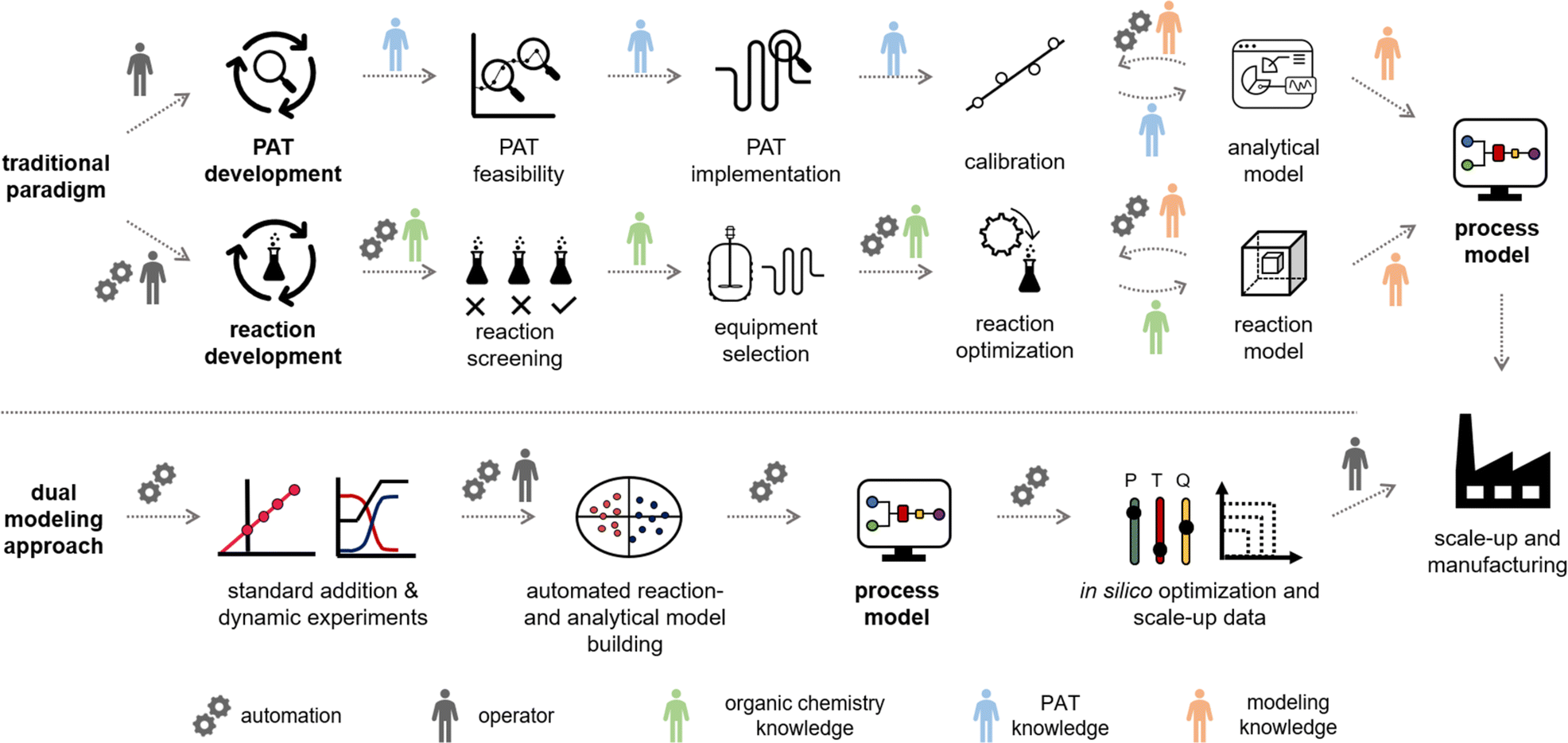Fig. 1 Top: Example of a traditional optimization approach for process development. Typically, the reaction and the PAT models are developed separately by several team members with different background knowledge. Bottom: The dual modeling approach, utilizing a high degree of automation to combine PAT and reaction optimization, resulting in a full process model.

Despite the range of advanced methods available, many reactions, particularly in flow, are still optimized by changing one variable at a time (OVAT) with offline analysis of the results.⁷ Automation, data-rich experiments and real-time process analytics can drastically accelerate development and collect process-relevant data quickly and efficiently.^13–15 Self-optimization and automated Design of Experiments (DoE) have been proven to be excellent methodologies for screening a broad process space and finding optimal process conditions.^16–21 The material consumption for these optimization methodologies can be drastically reduced by the use of droplet or slug flow platforms.^22–25

Kinetic models, due to their physics-based nature, generally provide more useful information on the reaction than empirical models, such as response surfaces generated from DoE experiments. Therefore, their use is preferred for process modeling, particularly for flow processes, which benefit from knowledge of reaction progress in both space (along the reactor) and time. Numerous platforms have been developed to establish and parameterize kinetic models using data generated in flow, but these either focus on a specific reaction type (not applicable to general synthetic organic chemistry),^26,27 use relatively simple data-processing methods (pre-developed chromatography methods or spectroscopy considering only a single peak),^28–31 or require a high degree of manual data processing.^32–36

The aforementioned kinetic model parameterization platforms generally rely on single data points, which are measured once the reactor has reached steady state. Utilizing dynamic experiments can drastically accelerate the collection of dense datasets.³⁷ In these experiments, ramps over time are executed to explore the design space. This dynamic change is followed with process analytical technology (PAT) and the collected data must be time-adjusted to match the corresponding input setpoints. Several approaches have been described in the literature in recent years, including ramps for a single process variable (often residence time)^29,38,39 or multiple process variables simultaneously.^40–48 Of these examples using dynamic experiments for kinetic model generation, additional offline work was required to obtain accurate concentration values from complex reaction mixtures.

The implementation of PAT and data processing models is still a substantial hurdle for non-specialist chemists.^49–51 This typically requires expert knowledge to develop and calibrate data processing (chemometric) models, in a time- and resource intensive procedure. Automating the workflow for collection, data processing and model generation from dynamic experiment data will drastically accelerate process development timeframes.

The use of data-rich workflows also plays an important role in advancing sustainability and green practices across the pharmaceutical industry. There exists a large number of sustainable synthesis procedures that do not receive their warranted attention, often due to a lack of data and understanding around their operation and broader applicability. An excellent example of such a methodology is the 1,5,7-triazabicyclo[4.4.0]dec-5-ene (TBD)-catalyzed amidation of esters,^52–55 which obviates an ester hydrolysis step and the use of a stoichiometric coupling agent.^56,57 To increase uptake of such sustainable synthesis methodologies, data-rich experimentation facilitates rapid scoping, allowing chemists to make informed, data-driven decisions. Real-time monitoring and advanced data analytics can then accelerate process optimization and the development of science-based control strategies, which secure medicine supplies and prevent waste in manufacturing.

To fulfill all of these requirements, we endeavored to establish a platform that calibrates process analytics, collects optimization data in a dynamic flow regime, and parameterizes a process model for scale-up in less than a working day (<8 h, Fig. 1, bottom). This optimization platform has a high degree of automation, but still includes the operator in the loop. The calibration of PAT is performed using a standard addition approach⁵⁸ in continuous flow. The standard addition data trains a partial least squares (PLS) regression model for species quantification. This model is then applied to the collected dynamic flow experiment data in a broad process space. The processed analytical data is fed with all process inputs into a software program, which is coded in Julia. The program is capable of fitting kinetic parameters and creating a process model that can be used for in silico optimization and to guide scale-up. The developed workflow is showcased with a broad scope of amidation reactions between esters and amines and the two-step synthesis of the API benznidazole (alkylation followed by amidation).

Results and discussion

Platform and approach

In traditional process development, reaction models are built mainly using data from offline analysis (Fig. 1, top). This workflow includes the initial reaction screening and feasibility study, reaction optimization and the reaction model development. In parallel to (or even after) the reaction development, a PAT and control strategy is often developed to control critical quality attributes (CQAs) in the final process. This encompasses the feasibility and implementation of PAT within the process, calibration of the process analytics, and the real-time processing of raw data into meaningful information (e.g., species concentrations and performance metrics). Multiple scientists with individual expertise will work on both workflows to combine them into a final process model. The digitalization of chemical development work provides opportunities to automate parts of the aforementioned workflows. This ultimately will save resources and accelerate the development of processes.

The proposed “dual modeling approach”, detailed in this manuscript, combines the development of a PAT strategy and reaction optimization in one synergistic workflow. This highly digitalized workflow is separated into two parts, which are simultaneously executed on one platform (Fig. 1, bottom). The platform can be comprised of any flow chemistry equipment and different process analytics. A degree of automation is necessary to send new setpoints to the flow equipment over pre-determined time intervals. To follow this precise workflow, two valves should be present in the setup, allowing the reactor to be bypassed, dosing the product to the reaction stream before or after the reactor. This allows for maximum flexibility in terms of quick PAT calibration and investigation of the reaction design space.

A standard addition approach in continuous flow is utilized to calibrate the PAT. Similar to a batch standard addition,^58–60 different concentration levels are measured by varying the pump flow rates accordingly. Bypassing the reactor enables steady-state conditions to be reached rapidly, facilitating fast acquisition of the concentration level data. Product calibration is achieved by continuously spiking a known concentration of product to the reactor outlet.

The standard addition is utilized to assign concentration values to each recorded spectrum. The labelled spectra with concentration values are then used to train and validate a PLS regression model. The PLS model is generated within this workflow through either automated means using a Python program or by an operator using chemometrics software (in our case PEAXACT software from S-PACT).

Dynamic experiments are automatically executed after the calibration stage to explore the reaction design space. Different reaction conditions are explored with single parameter- or multiple parameter ramps. Steady states between the dynamic ramps facilitate the data evaluation and act as points of validation in the results.

Process models from the acquired dynamic experiments are generated using software coded in the programming language Julia. Julia focuses on scientific computing, data analysis and statistical programming.⁶¹ It is an open-source programming language and utilizes precompiled code, which accelerates the execution of the code. The developed software fulfills the data handling, the definition of the chemical reactor, the identification of kinetic parameters, and performs in silico optimization with the generated process model within minutes.

The input parameters from the reactor and measured concentration values from the dynamic experiments are read by the software. The operator has only to define the reaction network and the reactor configuration in the software. The kinetic parameters are fitted by employing a cost function, which compares the measured results to the computed results from the kinetic parameters and inputs. A global optimization algorithm (NLopt-BOBYQA)⁶² is employed to find the global best fit for the kinetic parameters. The global optimum is then refined using a simplex algorithm (Nelder–Mead). The obtained kinetic parameters are combined into a process model, which can be used for in silico optimization, such as identifying the Pareto front of competing objectives or simulating any other point of interest.

Dual modeling for sustainable amidation

The formation of an amide bond is one of the most important reactions in the pharmaceutical industry.^56,57,63 TBD has been shown to be an effective catalyst in facilitating the amidation of esters by primary and secondary amines (Fig. 2A), including demonstration on >10 kg scale.^52–55,64 Despite its tremendous potential in improving sustainability, TBD-catalyzed amidation has received surprisingly little attention. Accordingly, this provides a perfect opportunity to incorporate a data-rich workflow for reaction optimization and understanding of substrate effects. Continuous flow processing can act as an enabling technology to apply high pressure and temperature and intensify the reaction. In our investigation, combinations of 5 esters (1a–e) and 3 amines (2a–c) were examined with this dual modeling approach.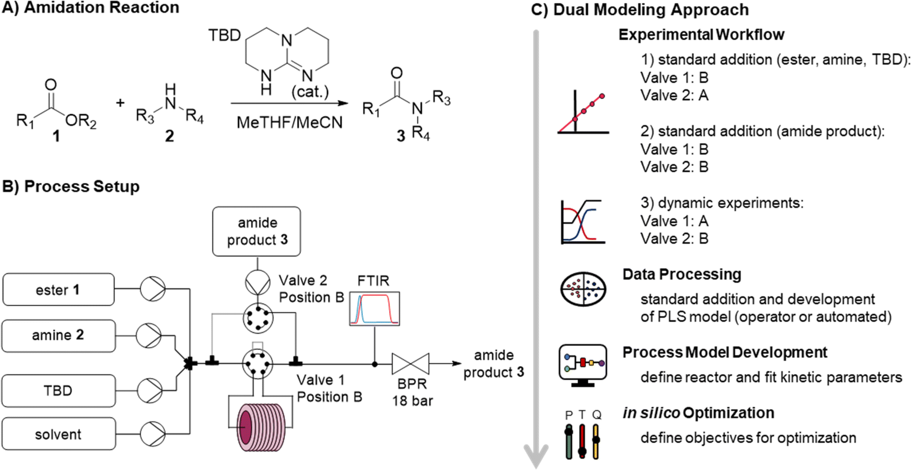

Fig. 2 (A) General reaction scheme of the investigated TBD-catalyzed amidation reaction. (B) The optimization platform used to perform the dual modeling approach. (C) The automated workflow of the dual modeling approach.

The continuous flow setup was comprised of commercially available flow equipment, automated and controlled with an orchestrating software (Fig. 2B). In order to minimize the void volume of the transfer lines, polytetrafluoroethylene (PTFE) tubing with an inner diameter of 0.3 mm was utilized. The feed solutions of ester, amine, TBD, solvent, and the amide product were prepared in MeTHF/MeCN (9 + 1 v/v) and introduced by HPLC pumps. The ester, amine, TBD and solvent feeds were mixed in a 7-port mixing unit (with 2 blocked ports). An automatic 6-port valve (valve 1) was utilized to either (position A) direct the reaction mixture through a stainless steel reactor coil (5.67 mL, 0.8 mm i.d.) placed on a heating block or (position B) guide it directly to a Fourier transform infrared spectrometer (FTIR). Another automatic 6-port valve (valve 2) was used for calibration purposes, to dose the amide product either directly before the reactor (position A) or after the reactor (position B) via a T-piece. The system was pressurized with a membrane-based back-pressure regulator (set to 18 bar).

The experimental workflow for the calibration of the FTIR was automatically executed and a standard addition approach was used. First, 6 different levels of ester, amine, TBD and solvent were generated and directly analyzed by FTIR, without passing through the reactor (Fig. 3A). The product standard addition was performed by allowing a certain reaction composition to pass through the reactor, then dosing 6 different concentrations of product to the outcoming reaction mixture (Fig. 3B). The assignment of the concentration values with the standard addition is outlined in detail in the ESI.†

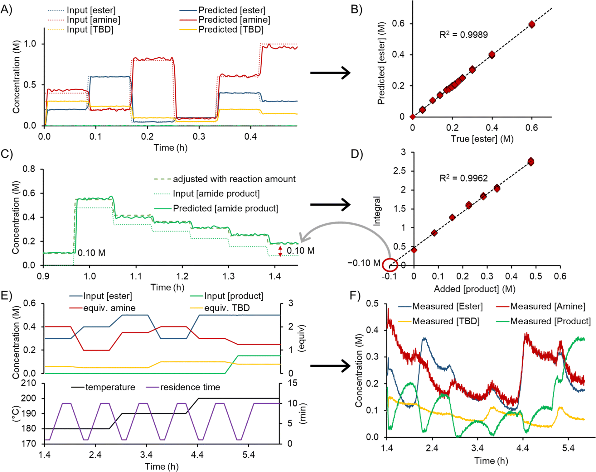Fig. 3 (A) 6 different concentration levels for ester, amine, TBD to obtain data for training the PLS model. (B) Representative parity plot for the generated ester PLS model including the R² statistic. (C) Representative graph for the amide product standard addition. (D) Concentration values for the standard addition of amide product. (E) Pre-determined process parameter ramps over time for the dynamic experiments. (F) Representative graph showing the FTIR-measured concentration values for ester, amine, TBD, and amide product from the PLS model during the dynamic experiment.

Each calibration level operated for a duration of 3 minutes and necessitated the consumption of the following quantities: 9.4 mL of 2.5 M ester solution (24 mmol), 16.3 mL of 2.5 M amine solution (41 mmol), 6.9 mL of 1.5 M product solution (10 mmol), 26.3 mL of 0.5 M base solution (13 mmol), and 30.8 mL of solvent. The operation of 3 minutes for each concentration level allowed 18–20 FTIR spectra to be measured (15 s acquisition time per spectrum). Further decreasing the material consumption could be achieved by shortening the run time for each concentration level, resulting in fewer spectra. A quantity of ≤5 spectra per concentration level should be sufficient to build a PLS model, thereby consuming only a quarter of the aforementioned amounts. If necessary, this quantity could be even further reduced by lowering flow rates, or even stopping the flow to allow additional time within the FTIR flow cell. However, it should be kept in mind that complete mixing of the input streams must be ensured by the time the mixture reaches the analysis point.

The amine pump was also turned off during the standard addition process to investigate if an intermediate species between the ester and the TBD could be observed, with or without passing through the heated reactor coil (Valve 1 in position A or B). In each case, no significant decrease in the ester concentration was observed, implying that the active intermediate does not form (in appreciable quantities) in the absence of an amine nucleophile. This is in agreement with previous reports, whereby the formation of an acylated TBD intermediate is reversible⁶⁵ and has only been isolated in reaction with specific lactone substrates.⁶⁶

In theory, low level impurities could also be calibrated using standard addition workflow. This is often used in analytical chemistry methodologies using quantification methods with ICPMS, UV/vis, etc. However, low-level impurities cannot be accurately detected/quantified with FTIR. This is due to the overlapping peaks and low sensitivity of the FTIR. The limit of detection for FTIR is generally in the range of 10–20 mM, depending on the other components and signal intensities.

Two methods of building a PLS model were investigated: (1) automated PLS model generation in Python and (2) manual PLS model generation in PEAXACT (by an operator). Typically, 12 different concentration levels from the standard addition were used as training data for the PLS model. Both approaches provide similar results, however the automated approach reduced the PLS model generation time from an hour (depending on experience of the user) to a few minutes. Applying a first derivative pretreatment to the raw spectra provided improved results compared to second derivative or no derivative. Multiple PLS models were generated for the different substrate combinations with both processing approaches. The obtained results (ranks for the PLS model, RMSEs and mass balances) from both approaches provided similar results and are explained in detail in the ESI.†

The root mean square error of cross validation (RMSE_CV) for the different esters 1, amines 2, TBD and the formed amide products 3 were between 18–68 mM, 30–214 mM, 9–50 mM, and 12–42 mM, respectively. In most dynamic flow experiments, the relative error for the mass balance of ester and amine was below 10%, which is within the uncertainty of the PLS model. In almost all experiments a higher error in mass balance was observed for TBD. Predictions for the amine typically had more noise compared to product and ester predictions. This might be explained by limited characteristic bands in the spectrum (only two bands observed in the fingerprint region below 800 cm⁻¹) for the amine substrates.

The dynamic experiments were executed as a set of 6 different experimental points (Fig. 3C) to explore a broad chemical space. Three different temperature levels (180 °C, 190 °C, and 200 °C) were investigated, with two dynamic ramp sets for each. The ester concentration was varied between 0.3 M and 0.5 M. The equivalents of amine and TBD were varied between 1.0–2.0 and 0.25–0.50, respectively. Product inhibition was investigated in the last experiment by adding 0.15 M (0.3 equivalents) of product to the reaction mixture. At the beginning of the dynamic experiment the system was equilibrated to steady state (for 5 min) with a residence time of 1 min. Then, a residence time ramp over 15 min was executed, from the shortest residence time of 1 min to the longest of 10 min. At the end of this ramp, the system was allowed to reach steady state again for 10 min. Then, the change to the next set of reaction conditions was achieved by dynamically changing all reaction parameters (residence time, temperature, equiv. amine, equiv. TBD, and concentration of ester) over 15 min. The resulting experimental program consisted of 4.5 h, resulting in a total time of 6 h, when combined with the initial calibration/standard addition levels.

The input data and processed FTIR data from the dynamic runs were saved in a standard spreadsheet file format by the operator, then moved to the correct directory to be read by the developed software in Julia (Fig. 4). The timestamps of the process parameters and measurement points were automatically interpolated to a uniform time axis. The operator must simply define the reactor setup (volume) in the software. In our case the reactor setup was comprised of two different segments. The first segment was the heated reactor part and the second segment was the tubing to the measurement point. Another input for the software is the reaction network. The change of reaction component concentrations, as a function of the transport and the kinetics, can be simulated with differential equations. Different global optimizers have been tested and the NLopt-BOBYQA algorithm was found to be most favorable in terms of performance and speed (see ESI†). Additionally, the refinement of the optimized parameters is achieved using a Nelder–Mead algorithm. The boundaries for the refinement are within +5% to −5% of the obtained global optimum.

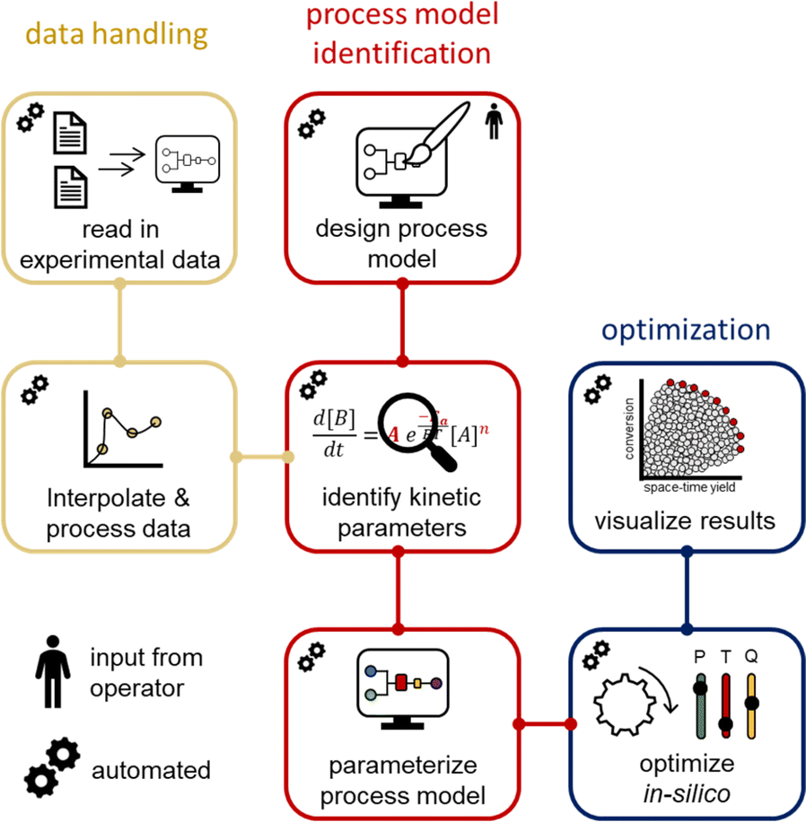Fig. 4 Schematic overview of the software developed in Julia. Data is automatically read in, interpolated and processed. Based on a process model (designed by an operator), the kinetic parameters are identified and a model parameterized. Using this model, in silico optimization can be performed.

The reaction kinetic parameters were fitted with a single- and two-step reaction network (Fig. 5A). The developed Julia software is able to fit reaction orders, the Arrhenius pre-exponential factor (A) and activation energy (E_A). For better comparison between each amidation reaction a two-step reaction network was used and the reaction orders were fixed to 1 for ester, amine, TBD and intermediate. In the first reaction the ester is activated by TBD to form an active N-acyl intermediate. This intermediate then reacts with the amine to the corresponding amide product, regenerating TBD.

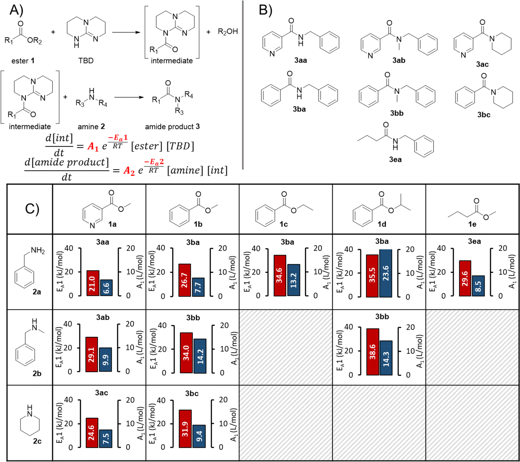Fig. 5 (A) Reaction network and equations used to fit kinetic parameters for the amidation reactions. (B) The formed amide products in the amidation reactions. (C) Pre-exponential factors in blue and activation energies in red for the first step of the amidation reactions with different ester and amine starting materials.

It should be noted that the aim of this investigation was not to ensure a mechanistically-accurate model, but to build simple and highly useable predictive models for optimization purposes. Accordingly, this relatively simple mechanism made the assumption that no side products were formed, since no major unexpected species were observed during initial trial reactions. The first reaction step (activation of the ester to form the N-acyl TBD intermediate) was assumed to be rate limiting, since the initially-fitted E_A parameters were significantly higher for this step than the second.

In general, a good fit of the kinetic model was achieved with all substrate combinations. However, for less reactive substrates (e.g., 1d + 2b) only a minor extent of product formation was observed. As a result, the product quantification using the PLS model had a large relative error, which had a knock-on effect to the kinetic model fitting for all concentration values. For other use cases, this should not be problematic, since the user will be most interested in reaction conditions that form a higher product concentration, while reactions will likely be abandoned if product formation is too low for accurate quantification. Details and parity plots for all kinetic model fits can be found in the ESI.†

In total 10 different amidation reactions were investigated, including a comparison of different benzoic esters: methyl vs. ethyl vs. isopropyl ester (Fig. 5B). The activation energy (E_A1) and pre-exponential factor (A₁) for the activation of ester (step 1) are displayed in Fig. 5C. The corresponding activation energy values fitted for the second step (E_A2) were substantially lower in all cases, implying that the first step was rate limiting. Accordingly, the values fitted for step 1 were used to compare different reactivities. Although this cannot be confirmed, it does make mechanistic sense, since the N-acyl intermediate concentration was not observable for any of the tested substrates.

The activation energy for the reaction of pyridine-based ester 1a with the different amines 2a, 2b and 2c was 21.0 kJ mol⁻¹, 29.1 kJ mol⁻¹, and 24.6 kJ mol⁻¹, respectively. This reactivity follows a trend for amine nucleophiles: primary > cyclic secondary > acyclic secondary (2a > 2c > 2b). The same order of reactivity was also observed for carbocyclic ester 1b. Activation energies of 26.7 kJ mol⁻¹, 34.0 kJ mol⁻¹, and 31.9 kJ mol⁻¹ were fitted for its reaction with 2a, 2b and 2c, respectively. Although the reactivity order of cyclic vs. acyclic secondary amines follows known nucleophilicity scales, the primary amine would be expected to be less reactive.⁶⁷ This implies that other factors, such as steric effects or hydrogen bonding capabilities, have an increased influence in this reaction.

The electron-deficient nature of heterocyclic ester 1a significantly enhanced the reaction rate compared to carbocyclic ester 1b. The increased reactivity was reflected in the lower activation energies for 1a in reactions with all three different amines. This is in agreement with the reported large positive Hammett substituent constant for a 3-pyridyl substituent (σ = +0.55).⁶⁸

A slightly lower activation energy of 26.7 kJ mol⁻¹ was obtained for 1b compared to 1e (29.6 kJ mol⁻¹) in the reaction with 2a, quantifying the difference in reactivity between aromatic and aliphatic esters. By means of comparing the influence of the alkoxy group on ester reactivity, the methyl moiety (1b) had a lower activation energy than ethyl (1c), which was lower than the sterically bulky isopropyl group (1d). Although this trend would be expected (methyl > ethyl > isopropyl), we have quantified the relationship between these esters. Interestingly, this study has also demonstrated that the reactivity of both the amine and ester partners are of key importance to achieving successful reaction, which is not immediately intuitive when considering the mechanism proceeding via a TBD N-acyl intermediate.

Finally, we have also demonstrated that the kinetic parameter fitting is not restricted to a specific set of experimental setpoints. This was evidenced by the fact that similar kinetic parameters were obtained for the reaction of 1a with 2a in a dynamic experiment using different (less forcing) experimental setpoints (see ESI† Section 6.2 vs. Section 6.12). Although it would be assumed that the kinetic model would be less applicable to conditions outside of its initial boundaries, this implies that its predictive nature remains relevant over a broader range.

Application to API synthesis

To examine and demonstrate the dual modeling approach further, the two-step synthesis of an API was performed. Benznidazole (7) is used for the treatment of Chagas disease (American trypanosomiasis) and is on the World Health Organization (WHO) list of essential medicines.⁶⁹ The API can be synthesized by alkylation of 2-nitroimidazole (4) with ethyl bromoacetate (5) to form ethyl ester 6 (Fig. 6A), followed by TBD-catalyzed amidation with benzylamine (2a) (Fig. 6C). Both transformations would benefit in terms of process intensification by developing a continuous flow protocol. The alkylation step also provides an opportunity to demonstrate the utility of the dual modeling approach for a different reaction type.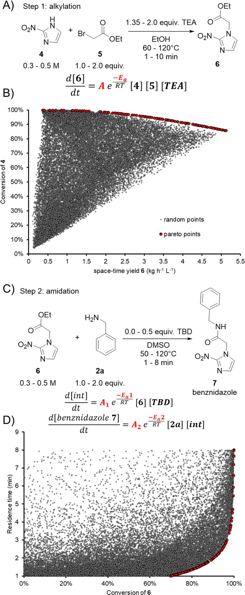

Fig. 6 (A) Reaction scheme for the alkylation step yielding ethyl ester 6. (B) NSGA-II optimization to determine the Pareto optimal front, balancing the trade-off between conversion and space-time yield. Pareto optimal front depicted by red points, contrasting with gray points (from random inputs). (C) Reaction scheme for the amidation yielding benznidazole 7. (D) Visualization of residence time vs. conversion. Pareto optimal front depicted by red points, contrasting with gray points (from random inputs).

The alkylation step was carried out in a similar setup as described for the aforementioned amidation reactions. The feed solutions of 4, 5, triethylamine (TEA) and 6 were prepared in ethanol. The solubility of 4 was increased by adding 1.1 equiv. TEA to the stock solution. The reactor coil was switched to a 2.79 mL perfluoroalkoxy alkane (PFA) coil and the BPR was set to 18 bar. During the dynamic experiments for the alkylation step, the concentration of 4 was varied between 0.3 and 0.5 M and the temperature was varied between 60 and 120 °C. The loading of 5 and TEA were varied between 1.0–2.0 and 1.35–2.0 equivalents, respectively. The residence time ramps were between 1 and 10 minutes.

Using the same workflow described above, the FTIR calibration was performed by the standard addition approach, prior to performing dynamic experiments. The auto-generated PLS model had a RMSE_CV of 43 mM, 42 mM, 18 mM, and 46 mM for 4, 5, TEA, and 6, respectively. This PLS model was applied to the dynamic run, then the process parameters and FTIR results were fed into the Julia software. The kinetic parameters were fitted as a trimolecular single step reaction, with fixed reaction orders of 1 for 4, 5 and TEA. The fitted pre-exponential factor (A) was 1.986 × 10⁵ L² mol⁻² with an activation energy (E_A) of 49.5 kJ mol⁻¹. The activation energy in this case was higher than that of all previously-examined amidation reactions, meaning that the rate of the alkylation has a comparatively higher temperature-dependence.

Another advantage of building a process model, such as this, is the opportunity to perform further in silico optimization. As an example, optimization was performed using the NSGA-II algorithm to find a Pareto front of the two opposing objectives: conversion and space-time yield (Fig. 6B). Points in red show the Pareto front, which is a series of optimal points showing the trade-off between the two objectives. A large number of random results (gray points) were also generated to demonstrate that none of these would surpass the Pareto front. Following this optimal front, a maximum space-time yield of 3.2 kg L⁻¹ h⁻¹ of 6 can be achieved when ensuring conversion >95%. Should a higher conversion of >99% be required, a maximum space-time yield of 1.9 kg L⁻¹ h⁻¹ of 6 would be attainable. It should be noted that this type of analysis can readily be carried out for any desired combination of objectives. The corresponding process setpoints can be obtained and utilized in future experiments.

In the amidation step the feed solutions of 6, 2a, TBD and 7, were prepared in DMSO, due to poor solubility in the previously-used MeTHF/MeCN solvent system. The same reactor setup was used as for the previous reaction step. The dynamic runs screened the following chemical space: 0.3–0.5 M of 6, 1.0–2.0 equiv. 2a, 0.0–0.5 equiv. TBD, temperature 50–120 °C, and residence time 1–8 min. In the last experimental point, the concentration of TBD was completely omitted to confirm that no reaction was observed.

The PLS model for the FTIR measurements to follow the dynamic runs was developed with the previously described methodology. The RMSE_CV for the compounds 6, 2a, TBD, and 7 were 24 mM, 33 mM, 11 mM, and 28 mM, respectively. The kinetics for the amidation step were fitted with the same reaction mechanism as described above (Fig. 5A). The following kinetic parameters for the first step (intermediate formation) were fitted: A₁ = 7.524 L mol⁻¹ and E_A1 = 14.19 kJ mol⁻¹. In the second step (formation of product), the best-fitting parameters were: A₂ = 6.659 L mol⁻¹ and E_A2 = 11.5 kJ mol⁻¹.

The optimal operating space (Pareto front) was identified using an in silico multi-objective optimization for residence time and conversion (Fig. 6D). It can be observed that residence times of 4.25 min can still provide conversion >99% with a space-time yield of 1.8 kg L⁻¹ h⁻¹. Increasing the space-time yield to 2.8 kg L⁻¹ h⁻¹ results in a decrease of residence time to 2.6 min, providing 95% conversion.

Conclusion

In summary, we have developed and demonstrated a holistic “dual modeling” approach to reaction optimization. This approach is capable of developing both an analytical model and reaction model within one experimental day. First, standard addition is utilized to collect calibration data for the FTIR and a python program automatically generates a PLS model to determine species concentrations. Dynamic flow experiments are then used to quickly cover a broad chemical space and collect high density data for reaction model development. The obtained data is fed into a software program that fits kinetic parameters for different reaction networks within minutes. Additionally, the software can use the fitted kinetic parameters and the reactor geometries to generate a digital twin of the synthesis process. This process model is utilized for in silico optimization of multiple objectives, such as conversion, space-time yield or measures of environmental impact. This level of automation and integration has not before been shown in related studies and drastically reduces optimization timescales, saving resources during process development.

This dual modeling approach was applied to a rarely-used protocol for sustainable amidation reactions. By examining a range of different substrate combinations, insights into the different kinetics for each substrate were gained. Accordingly, a better understanding of the compatible reaction substrates can be inferred. We then expanded this approach to the two-step synthesis of the API benznidazole, where both the alkylation and amidation reactions proved to be amenable to this approach. The developed reaction models were also utilized for in silico optimization, whereby different objectives, and the trade-offs between them, can be rapidly explored without additional experimental effort. Such straightforward transferability different reaction systems, without prior work required, and general applicability to organic synthesis problems represents a significant advantage compared to previous workflows.

Following on from this initial dissemination, we expect the dual modeling approach to be utilized in a wide range of future studies. For example, the method can be used to rapidly determine the Hammett reaction constant, ρ, for new synthetic methodologies and sustainable alternatives, providing predictable applicability for different substrate classes. Furthermore, we anticipate exploration of additional PAT instruments, such as chromatographic analysis, to provide more insight into impurities and allow more precise quantification of reaction intermediates. Different and more complex reaction kinetics, such as catalytic cycles, can also be modeled using this approach, by simply adjusting the reaction networks written into the Julia software. Bespoke Julia packages (e.g., catalyst.jl) can be utilized for this purpose.

Data availability

The developed Julia code for this study can be found at: https://github.com/SagmeisterPeter/Julia-Kinetics.

Author contributions

JDW and PS conceived the study. PS developed the methodology. LM and PS performed experiments and analyzed the data. JDW and COK acquired funding and provided project supervision. JDW and PS wrote the original draft of the paper. All authors contributed to the final manuscript.

Conflicts of interest

There are no conflicts to declare.

Acknowledgements

This manuscript was developed with the support of the American Chemical Society Green Chemistry Institute Pharmaceutical Roundtable (https://www.acs.org/content/acs/en/greenchemistry/industry-business/pharmaceutical.html). The ACS GCI is a not-for-profit organization whose mission is to catalyze and enable the implementation of green and sustainable chemistry throughout the global chemistry enterprise. The ACS GCI Pharmaceutical Roundtable is composed of pharmaceutical and biotechnology companies and was established to encourage innovation while catalyzing the integration of green chemistry and green engineering in the pharmaceutical industry. The activities of the Roundtable reflect its members' shared belief that the pursuit of green chemistry and engineering is imperative for business and environmental sustainability. The Research Center Pharmaceutical Engineering (RCPE) is funded within the framework of COMET–Competence Centers for Excellent Technologies by BMK, BMAW, Land Steiermark and SFG. The COMET program is managed by the FFG. The authors thank Dr Markus Tranninger and Patrick Frisinghelli for discussion and assistance during the Julia software development.

Notes and references

1. S. V. Ley, D. E. Fitzpatrick, R. J. Ingham and R. M. Myers, Angew. Chem., Int. Ed., 2015, 54, 3449–3464.
2. C. Allais, C. G. Connor, N. M. Do, S. Kulkarni, J. W. Lee, T. Lee, E. McInturff, J. Piper, D. W. Place, J. A. Ragan and R. M. Weekly, ACS Cent. Sci., 2023, 9, 849–857.
3. A. S. Anderson, Nat. Med., 2022, 28, 1538.
4. B. Halford, ACS Cent. Sci., 2023, 9, 1715–1717.
5. B. Halford, ACS Cent. Sci., 2022, 8, 405–407.
6. C. W. Coley, D. A. Thomas, J. A. M. Lummiss, J. N. Jaworski, C. P. Breen, V. Schultz, T. Hart, J. S. Fishman, L. Rogers, H. Gao, R. W. Hicklin, P. P. Plehiers, J. Byington, J. S. Piotti, W. H. Green, A. J. Hart, T. F. Jamison and K. F. Jensen, Science, 2019, 365, eaax1566.
7. C. J. Taylor, A. Pomberger, K. C. Felton, R. Grainger, M. Barecka, T. W. Chamberlain, R. A. Bourne, C. N. Johnson and A. A. Lapkin, Chem. Rev., 2023, 123, 3089–3126.
8. J. Britton and C. L. Raston, Chem. Soc. Rev., 2017, 46, 1250–1271.
9. M. B. Plutschack, B. Pieber, K. Gilmore and P. H. Seeberger, Chem. Rev., 2017, 117, 11796–11893.
10. B. Gutmann, D. Cantillo and C. O. Kappe, Angew. Chem., Int. Ed., 2015, 54, 6688–6728.
11. M. Baumann, T. S. Moody, M. Smyth and S. Wharry, Org. Process Res. Dev., 2020, 24, 1802–1813.
12. C. P. Breen, A. M. K. Nambiar, T. F. Jamison and K. F. Jensen, Trends Chem., 2021, 3, 373–386.
13. G. Schneider, Nat. Rev. Drug Discovery, 2018, 17, 97–113.
14. A. M. K. Nambiar, C. P. Breen, T. Hart, T. Kulesza, T. F. Jamison and K. F. Jensen, ACS Cent. Sci., 2022, 8, 825–836.
15. P. Sagmeister, J. D. Williams and C. O. Kappe, Chimia, 2023, 77, 300–306.
16. A. M. Schweidtmann, A. D. Clayton, N. Holmes, E. Bradford, R. A. Bourne and A. A. Lapkin, Chem. Eng. J., 2018, 352, 277–282.
17. P. Sagmeister, F. F. Ort, C. E. Jusner, D. Hebrault, T. Tampone, F. G. Buono, J. D. Williams and C. O. Kappe, Adv. Sci., 2022, 9, 2105547.
18. A. D. Clayton, E. O. Pyzer-Knapp, M. Purdie, M. F. Jones, A. Barthelme, J. Pavey, N. Kapur, T. W. Chamberlain, A. J. Blacker and R. A. Bourne, Angew. Chem., Int. Ed., 2023, 62, e202214511.
19. P. Jorayev, D. Russo, J. D. Tibbetts, A. M. Schweidtmann, P. Deutsch, S. D. Bull and A. A. Lapkin, Chem. Eng. Sci., 2022, 247, 116938.
20. P. Müller, A. D. Clayton, J. Manson, S. Riley, O. S. May, N. Govan, S. Notman, S. V Ley, T. W. Chamberlain and R. A. Bourne, React. Chem. Eng., 2022, 7, 987–993.
21. S. Knoll, C. E. Jusner, P. Sagmeister, J. D. Williams, C. A. Hone, M. Horn and C. O. Kappe, React. Chem. Eng., 2022, 7, 2375–2384.
22. A. Slattery, Z. Wen, P. Tenblad, J. Sanjosé-Orduna, D. Pintossi, T. den Hartog and T. Noël, Science, 2024, 383, eadj1817.
23. B. J. Reizman, Y. M. Wang, S. L. Buchwald and K. F. Jensen, React. Chem. Eng., 2016, 1, 658–666.
24. L. M. Baumgartner, C. W. Coley, B. J. Reizman, K. W. Gao and K. F. Jensen, React. Chem. Eng., 2018, 3, 301–311.
25. F. Wagner, P. Sagmeister, C. E. Jusner, T. G. Tampone, V. Manee, F. G. Buono, J. D. Williams and C. O. Kappe, Adv. Sci., 2024, 2308034.
26. S. G. Bawa, A. Pankajakshan, C. Waldron, E. Cao, F. Galvanin and A. Gavriilidis, Chem.: Methods, 2023, 3, e202200049.
27. A. Pankajakshan, S. G. Bawa, A. Gavriilidis and F. Galvanin, React. Chem. Eng., 2023, 8, 3000–3017.
28. S. Schwolow, F. Braun, M. Rädle, N. Kockmann and T. Röder, Org. Process Res. Dev., 2015, 19, 1286–1292.
29. C. A. Hone, N. Holmes, G. R. Akien, R. A. Bourne and F. L. Muller, React. Chem. Eng., 2017, 2, 103–108.
30. C. J. Taylor, M. Booth, J. A. Manson, M. J. Willis, G. Clemens, B. A. Taylor, T. W. Chamberlain and R. A. Bourne, Chem. Eng. J., 2021, 413, 127017.
31. E. Agunloye, P. Petsagkourakis, M. Yusuf, R. Labes, T. Chamberlain, F. L. Muller, R. A. Bourne and F. Galvanin, React. Chem. Eng., 2024, 9, 1859–1876.
32. V. Fath, P. Lau, C. Greve, N. Kockmann and T. Röder, Org. Process Res. Dev., 2020, 24, 1955–1968.
33. L. Schulz, P. Stähle, S. Reining, M. Sawall, N. Kockmann and T. Röder, J. Flow Chem., 2023, 13, 13–19.
34. O. Bortolini, A. Cavazzini, P. P. Giovannini, R. Greco, N. Marchetti, A. Massi and L. Pasti, Chem.–Eur. J., 2013, 19, 7802–7808.
35. J. S. Moore, C. D. Smith and K. F. Jensen, React. Chem. Eng., 2016, 1, 272–279.
36. M. Glace, W. Wu, H. Kraus, D. Acevedo, T. D. Roper and A. Mohammad, React. Chem. Eng., 2023, 8, 1032–1042.
37. J. D. Williams, P. Sagmeister and C. O. Kappe, Curr. Opin. Green Sustainable Chem., 2024, 47, 100921.
38. J. S. Moore and K. F. Jensen, Angew. Chem., Int. Ed., 2014, 53, 470–473.
39. J. Van Herck and T. Junkers, Chem.: Methods, 2022, 2, 1–6.
40. F. Florit, A. M. K. Nambiar, C. P. Breen, T. F. Jamison and K. F. Jensen, React. Chem. Eng., 2021, 6, 2306–2314.
41. B. M. Wyvratt, J. P. McMullen and S. T. Grosser, React. Chem. Eng., 2019, 4, 1637–1645.
42. B. Zhang, A. Mathoor and T. Junkers, Angew. Chem., Int. Ed., 2023, 62, 1–7.
43. C. Waldron, A. Pankajakshan, M. Quaglio, E. Cao, F. Galvanin and A. Gavriilidis, React. Chem. Eng., 2020, 5, 112–123.
44. L. Schrecker, J. Dickhaut, C. Holtze, P. Staehle, A. Wieja, K. Hellgardt and K. K. M. Hii, React. Chem. Eng., 2023, 8, 3196–3202.
45. P. Sagmeister, C. Schiller, P. Weiss, K. Silber, S. Knoll, M. Horn, C. A. Hone, J. D. Williams and C. O. Kappe, React. Chem. Eng., 2023, 8, 2818–2825.
46. K. Silber, P. Sagmeister, C. Schiller, J. D. Williams, C. A. Hone and C. O. Kappe, React. Chem. Eng., 2023, 8, 2849–2855.
47. S. Martinuzzi, M. Tranninger, P. Sagmeister, M. Horn, J. D. Williams and C. O. Kappe, React. Chem. Eng., 2024, 9, 132–138.
48. S. D. Schaber, S. C. Born, K. F. Jensen and P. I. Barton, Org. Process Res. Dev., 2014, 18, 1461–1467.
49. P. Sagmeister, R. Lebl, I. Castillo, J. Rehrl, J. Kruisz, M. Sipek, M. Horn, S. Sacher, D. Cantillo, J. D. Williams and C. O. Kappe, Angew. Chem., Int. Ed., 2021, 60, 8139–8148.
50. M. A. Morin, W. (Peter) Zhang, D. Mallik and M. G. Organ, Angew. Chem., Int. Ed., 2021, 60, 20606–20626.
51. M. Rodriguez-Zubiri and F.-X. Felpin, Org. Process Res. Dev., 2022, 26, 1766–1793.
52. C. B. Lan and K. Auclair, J. Org. Chem., 2023, 88, 10086–10095.
53. E. Fritz-Langhals, Org. Process Res. Dev., 2022, 26, 3015–3023.
54. F. J. Weiberth, Y. Yu, W. Subotkowski and C. Pemberton, Org. Process Res. Dev., 2012, 16, 1967–1969.
55. C. Sabot, K. A. Kumar, S. Meunier and C. Mioskowski, Tetrahedron Lett., 2007, 48, 3863–3866.
56. A. El-Faham and F. Albericio, Chem. Rev., 2011, 111, 6557–6602.
57. J. R. Dunetz, J. Magano and G. A. Weisenburger, Org. Process Res. Dev., 2016, 20, 140–177.
58. G. Hutchinson, C. D. M. Welsh and J. Burés, J. Org. Chem., 2021, 86, 2012–2016.
59. J. Liu, Y. Sato, F. Yang, A. J. Kukor and J. E. Hein, Chem.: Methods, 2022, 2, 1–8.
60. Y. Sato, J. Liu, A. J. Kukor, J. C. Culhane, J. L. Tucker, D. J. Kucera, B. M. Cochran and J. E. Hein, J. Org. Chem., 2021, 86, 14069–14078.
61. J. Bezanson, A. Edelman, S. Karpinski and V. B. Shah, SIAM Rev., 2017, 59, 65–98.
62. G. H. Negri, M. S. M. Cavalca, J. de Oliveira, C. J. F. Araújo and L. A. Celiberto, J. Control Autom. Electr. Syst., 2017, 28, 623–634.
63. S. D. Roughley and A. M. Jordan, J. Med. Chem., 2011, 54, 3451–3479.
64. M. A. Levina, M. V. Zabalov, V. G. Krasheninnikov and R. P. Tiger, React. Kinet., Mech. Catal., 2020, 129, 65–83.
65. M. K. Kiesewetter, M. D. Scholten, N. Kirn, R. L. Weber, J. L. Hedrick and R. M. Waymouth, J. Org. Chem., 2009, 74, 9490–9496.
66. B. G. G. Lohmeijer, R. C. Pratt, F. Leibfarth, J. W. Logan, D. A. Long, A. P. Dove, F. Nederberg, J. Choi, C. Wade, R. M. Waymouth and J. L. Hedrick, Macromolecules, 2006, 39, 8574–8583.
67. F. Brotzel, C. C. Ying and H. Mayr, J. Org. Chem., 2007, 72, 3679–3688.
68. J. H. Blanch, J. Chem. Soc. B, 1966, 937–939.
69. I. Losada Galván, J. Alonso-Padilla, N. Cortés-Serra, C. Alonso-Vega, J. Gascón and M. J. Pinazo, Expert Rev. Anti-Infect. Ther., 2021, 19, 547–556.

---

Footnote

† Electronic supplementary information (ESI) available: Further details of reaction setups, experimental results and NMR data. See DOI: https://doi.org/10.1039/d4sc01703j

---