 Open Access Article
Creative Commons Attribution 3.0 Unported Licence
A comparative study of transient flow rate steps and ramps for the efficient collection of kinetic data†
Linden
Schrecker
 a,
Joachim
Dickhaut
b,
Christian
Holtze
b,
Philipp
Staehle
b,
Marcel
Vranceanu
b,
Andy
Wieja
b,
Klaus
Hellgardt
c and
King Kuok
Hii
 *a
*a
aDepartment of Chemistry, Imperial College London, Molecular Sciences Research Hub, 82 Wood Lane, London W12 0BZ, UK. E-mail: mimi.hii@imperial.ac.uk
bBASF SE, 8 Carl-Bosch-Straße, 67056, Ludwigshafen, Rhein, Germany
cDepartment of Chemical Engineering, Imperial College London, Exhibition Road, South Kensington, London SW7 2AZ, UK
First published on 8th February 2024
Abstract
Transient cumulative flow rate varying methods have proven very effective for the collection of residence time series data for reactions in continuous flow. In this study, comparisons will be made between data collected from step changes and linear flow rate ramps, to inform method choice and minimise the complexity of automation and control needed to implement these methods, without compromising the quality of the data. Using two different analytical tools (in-line FTIR and on-line HPLC), the methods were compared in two different flow system configurations, and across three chemical reactions of increasing complexity. This work finds that the quality of the data collected using simpler step changes are comparable to that collected using more complex ramping methods, when performed in a reverse push-out (high to low flow rate) manner.
Introduction
Gathering reaction kinetics data is critical for the development of any chemical process affording mechanistic understanding and knowledge for scale up. Traditionally, kinetic studies were perceived to be laborious and require specialised knowledge and equipment. In recent years, however, the increasing variety and availability of ‘plug and play’ laboratory-scale analytical tools,1 boosted by advances in laboratory automation,2,3 kinetics analysis methods,4 and software,5,6 have substantially lowered the barrier for implementation. However, most kinetic experiments still require repetition to account for experimental and human error. This problem is especially acute for reactions performed in batch reactors, where mass and heat transfer limitations can hinder the evaluation of a reaction's intrinsic kinetics; the investigation of reaction kinetics in flow can mitigate these problems while improving efficiency.7–10Prior to the development of transient flow experiments, it was widely accepted that it is easier to collect kinetic data using batch reactors, compared to using steady state methods in flow.11 Although steady state methods provide more accurate reaction data, they are too time and material intensive, requiring the same reaction conditions to be established throughout the entire reactor volume, before a data point can be collected. In the past 15 years, the emergence of a diverse range of non-steady state (transient) flow approaches began to challenge this approach, vastly improving the time efficiency and data quality of kinetic experimentation by varying a reaction parameter continuously.9,12–19 In order for these new techniques to be adopted, however, significant benefits over batch experiments must be demonstrated. Early methods, involving switching on an energy source12 or changing the volume of the reactor,13 improved efficiency but lack generality. In comparison, cumulative flow rate changing methods (flow rate step changes and ramps) are easier to implement and more general, as reactions initialised by mixing reagents and/or heating can also be monitored.9,14,17
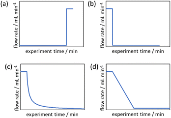
Cumulative flow rate step changes were first developed by Mozharov et al. in 2011 which were demonstrated to produce kinetic data five times faster than steady state methods.14 This work focused on “push-out” (PO) step changes in which the initial steady state is at a lower flow rate than the flow rate after the step change (Fig. 1a). Deviations were reported between the reaction data obtained from this method and steady state methods, purportedly due to the time taken for the flow rate to increase to the higher flow rate. Further comparison between PO step changes, “reverse push out” (RPO) step changes (high to low flow rate, Fig. 1b), and steady state methods was performed by Durand et al.15 This work noted that a PO step change is likely to have greater error than a RPO step change but uses less material, as the initial higher flow rate for a RPO step change requires a greater volume of solution to reach steady state. However, it was noted that RPO step changes, or smaller PO step changes, are useful when the sampling rate is a limitation.
Due to these perceived limitations of step change methods, cumulative flow rate ramping methods were developed. Generally the function of the flow rate ramp has been either a non-linear reciprocal function (Fig. 1c),17 in order to generate a linear residence time ramp, or linear (Fig. 1d),16 for ease of implementation. These ramps have generally been performed in a RPO type manner beginning at a high flow rate and gradually transitioning to a lower flow rate, producing a series of increasing reaction times mimicking batch experimental data. Cumulative flow rate ramps inherently use more material, more solvent, and take more time than cumulative flow rate step changes, and require greater pump control as the flow rate must be changed gradually. Flow rate ramps have become the norm by those skilled in the area as it is claimed the data produced are more accurate, however, no comparative study has been performed to justify this claim to warrant the use of these more complicated and less efficient flow rate ramps. Additionally, these more complex methods create a barrier-to-entry for those wishing to collect kinetic data which would be reduced by the use of step change methods.
To provide a useful comparison for both those utilising these techniques already and to facilitate their implementation by new users, in the following studies, comparisons are limited to simple methods that can be easily implemented with standard HPLC pumps. Although some HPLC pumps have the capability to perform non-linear flow rate ramps or can be remotely controlled, the methods were limited to linear flow rate ramps,16 both PO and RPO, as the most generally implementable. Linear residence time ramps (non-linear reciprocal flow rate ramps) were not compared as they require more specialised equipment and produce similar quality results to linear flow rate ramps, albeit with a more even distribution of time points.17
Results and discussion
Transient flow methods
Mathematically, all cumulative flow rate methods have the same underlying mathematical principles. As the cumulative flow rate is an integral parameter, the entire reactor volume is affected by a change in cumulative flow rate. Each differential volume element (or “slice”) of the reaction effluent must traverse through the volume of the reactor as propelled by the cumulative flow rate (Q). If this cumulative flow rate changes over the course of the experiment (Q(t), e.g. in transient flow) then this function must be integrated over the reactor volume (VR) between the time at which the slice enters the reactor (ti) and the time it exits the reactor (tf), which will give the residence time (τ) (eqn (1)–(3)). | (1) |
 | (2) |
 | (3) |
After exiting the reactor, there is often a dead volume before the analytical tool in which the reaction must be efficiently quenched to avoid further reaction, most simply by rapid cooling. In the same manner, this dead volume is also affected by the cumulative flow rate function, and can be evaluated similarly by integration of the dead volume (VD) between the time at which the slice exits the reactor (tf) and the measurement time (tm) (Fig. 2).
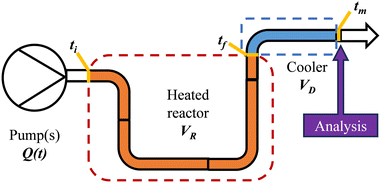 | ||
| Fig. 2 Diagrammatic representation of a generic flow reactor system with a dead volume between reactor and analysis device. | ||
The evaluation of the integral is dependent on the cumulative flow rate function(s) utilised. In the present work, this consists of either a step change, or a linear ramp (Fig. 3). Such flow rate functions have points of discontinuity at which the function changes, and thus these integrals must be separated at the points of discontinuity, such as at the step change itself. The direction of the flow rate change is either a push out (PO, from low to high flow) or a reverse push out (RPO, from high to low) method. Thus, in the following study, four transient flow methods will be evaluated as the cumulative flow rate function changing over the experimental time (Q(t)): (a) RPO step change, (b) PO step change, (c) RPO ramp, and (d) PO ramp.
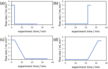 | ||
| Fig. 3 Example plots of cumulative flow rate functions with respect to experimental time for: (a) a RPO step change; (b) a PO step change; (c) a RPO ramp; (d) a PO ramp. | ||
 | (4) |
 | (5) |
Inclusion of dead volume terms in this evaluation facilitates application to more flow systems in which the analytical tool is not positioned directly after the flow reactor.
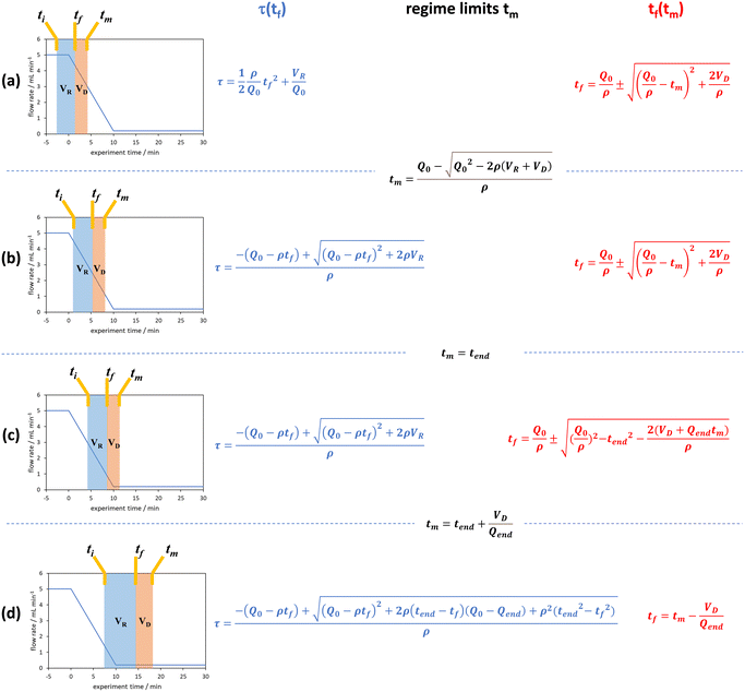 | ||
| Fig. 4 The graphical representation of the different regimes (a–d) where the integral of the blue area corresponds to the reaction volume and that of the red area to the dead volume. The corresponding blue and red equations refer to the conversion of tf to τ and tm to tf respectively. The black equations are the limits in which these regimes hold for a linear flow rate ramp, in this case demonstrated on the RPO ramp from Fig. 3c. | ||
In previous derivations of residence time from linear flow rate ramps, attempts were only made to extract a subset of these regimes, and any dead volume between the end of the reactor and the analytical device (VD, Fig. 2) was not accounted for.16 Although some work on linear residence time ramps did account for the dead volume, only a single flow rate function regime was evaluated.17 In this work, inclusion of all different regimes allows increased data to be obtained from a single experiment, compared to previous deconvolution methods.
Flow system configurations
The different methods were compared using two differently configured flow systems. Configuration 1 (Fig. 5a) has previously been described in our work,7 which was applied to the Knorr pyrazole synthesis reaction, and the hydrolysis of acetic anhydride. This configuration utilises an oil bath to control the temperature of the reaction and an in-line FTIR for reaction analysis. Configuration 2 (Fig. 5b) has also previously been described,8 for the aromatic Claisen rearrangement reaction. This configuration utilises an oven to control the temperature of the reaction and a custom on-line HPLC for reaction analysis (ESI† info).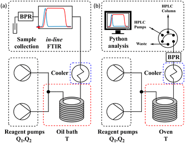 | ||
| Fig. 5 (a) Schematic of configuration 1 of the flow system utilising an oil bath and in-line FTIR; and (b) schematic of configuration 2 of the flow system utilising an oven and on-line HPLC. | ||
Results and discussion
Exemplars
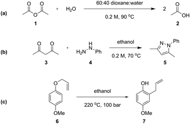
Three different chemical reactions (Scheme 1) were studied in this work, with varying levels of complexity: the hydrolysis of acetic anhydride, the condensation between pentane-2,4-dione and phenyl hydrazine (Knorr pyrazole synthesis), and the Claisen rearrangement of p-methoxyphenyl allyl ether. More detailed discussion of the kinetics of the Knorr pyrazole synthesis and aromatic Claisen rearrangement can be found in our previous work.7,8The hydrolysis of acetic anhydride 1 to acetic acid 2 (Scheme 1a) is an exothermic reaction widely used as a benchmark for testing calorimetric systems.20–22 In the presence of excess water, the pseudo-first order reaction is highly exothermic (ΔHrxn of −63 kJ mol−1 in water22), which can make accurate analysis challenging. Previously, kinetic data of this reaction has been collected in flow using a linear residence time ramp with in-line flow calorimetry.22 A mixture of 1![[thin space (1/6-em)]](https://www.rsc.org/images/entities/char_2009.gif) :
:![[thin space (1/6-em)]](https://www.rsc.org/images/entities/char_2009.gif) 4 dioxane and water was utilised, in order to maintain a homogeneous reaction mixture.23,24
4 dioxane and water was utilised, in order to maintain a homogeneous reaction mixture.23,24
The Knorr pyrazole synthesis is a double condensation reaction between a 1,3-diketone and a hydrazine to form the pyrazole heterocycle. The reaction kinetics of this reaction were previously studied in flow, performing an energy source ‘switch-on’ method to collect time series data to fit to a global rate law.12 The reaction between pentane-2,4-dione (3) and phenyl hydrazine (4) (Scheme 1b) was chosen for this study as it has a more complex reaction pathway than the hydrolysis of acetic anhydride.7
The aromatic Claisen rearrangement is a [3,3]-sigmatropic pericyclic rearrangement reaction, which is generally thermally activated (Scheme 1c). This reaction was chosen due to the first order reaction kinetics and extreme conditions (>200 °C) required, which benefit from the wider reaction space afforded by flow. This reaction has been studied kinetically in batch reactors in high boiling solvents, asserting the first order kinetics,25 in flow utilising steady state methods,26 and by us previously to demonstrate ‘one-pot’ transient flow methods.8
The hydrolysis of acetic anhydride and Knorr pyrazole reaction were performed with the flow reactor in configuration 1, analysing the reaction mixture by in-line FTIR (ESI† information). Kinetic data was recorded utilising different transient flow methods, between flow rates of 0.2–5 mL min−1, which afforded yields up to 99% and 75%, respectively, at a residence time of 20 minutes. The Claisen rearrangement of allyl ether 6 was performed with the flow reactor in configuration 2, analysing the reaction mixture by on-line HPLC (ESI† information). Kinetic data was collected utilising different transient flow methods, between flow rates of 0.1–1 mL min−1, which afforded yields up to 92% at a residence time of 32 min.
Acetic anhydride hydrolysis
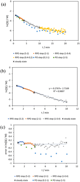
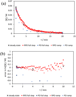
Initially, conversions were collected for individual steady state flow rates between 0.2–5 mL min−1, changing between each steady state by a well-defined cumulative flow rate step change (Fig. 6a). Averaged steady state conversion were calculated and a linear regression of the natural logarithm of acetic anhydride concentration was fitted, based on observed pseudo-first order kinetics, within the FTIR calibrated concentration range (above circa. 0.01 M, −4.6 on a ln([1]/M) scale) (Fig. 6b). This fitted data provided the benchmark to which different transient flow method data could be compared. This experiment also produced data for small RPO and PO step changes (Fig. 6c). These results showed very good agreement between averaged steady state values (black asterisks) and those obtained from the small RPO step changes (coloured diamonds). However, there was more error in the small PO step changes (coloured squares), potentially simply due to the larger change in flow rate performed in these cases.RPO and PO step changes were performed across the entire residence time range (red and blue dots, respectively, Fig. 7), between 5–0.2 mL min−1, maintaining the same step size for RPO and PO. Negligible deviation was observed for the RPO step change whereas the PO step change had greater error in the concentration measurements (average error in the natural logarithm of concentration (ε) of 0.09 cf. 0.65, Fig. 7b). Not only were the results from PO step changes less accurate, but they also produce significantly lower quantities of data, even with a relatively fast (15 seconds) analysis sampling time (in-line FTIR). In contrast, a PO linear flow rate ramp, applied upwards between 0.2–5 mL min−1 over 5 min (blue crosses, ε = 0.18) performed better than the full PO step change (blue dots, ε = 0.65) at short residence times but remained inaccurate in the rest of the flow rate range, albeit with more data points collected. A RPO linear flow rate ramp (downwards in flow rate, red crosses) afforded data that contain slightly less error (ε = 0.08) than the RPO full step change (red dots, ε = 0.09). These flow rate ramps have a similar ramp rate (∼1 mL min−2) to other linear flow rate ramps (cf. Hone et al. 10–1 mL min−1 over a 10 min ramp).16 A relatively fast ramp rate is desirable when utilising a fast analytical tool (FTIR scan rate of 15 s) to maximise method efficiency.
While the error associated with the RPO methods (coloured diamonds in Fig. 6, red dots and red crosses in Fig. 7) was more normally distributed, the error from PO methods (coloured squares in Fig. 6, blue dots and blue crosses in Fig. 7) tends toward greater conversions. This is presumably due to the delay in reaching a flow rate set point when increasing the flow rate, producing residence times consistently greater than those expected. Although error in the PO step change is present at all residence times, error in the PO ramp arises primarily at intermediary residence times, which might be explained by the cumulative effect of increasing flow rate: these intermediary data experience the flow rate changing for their entire residence time, and thus any small errors in changing flow rate to a faster flow rate (slight delays) will be most prominent in these data. In comparison, the data collected before and after the intermediary region will have experienced a fixed flow rate for some of their residence time and thus will have less error.
Knorr pyrazole synthesis
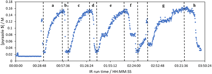
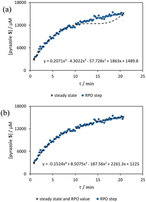
The comparison of residence time series collection methods for the Knorr pyrazole reaction was performed primarily in one continuous automated experiment (Fig. 8), in order to avoid variation in multiple solution preparation and system set up. This allows direct comparison between the different residence time collection methods. This experiment consisted of programming the HPLC pumps to deliver ramp rates in the following order: a) a full RPO step (5–0.2 mL min−1); b) a full PO step (0.2–5 mL min−1); c) a RPO ramp (5 min ramp, 5–0.2 mL min−1); d) a PO ramp (5 min ramp, 0.2–5 mL min−1); e) two consecutive smaller RPO steps (5–1 mL min−1 and 1–0.2 mL min−1), and; f) two consecutive smaller PO steps (0.2–1 mL min−1 and 1–5 mL min−1). At the end of this automated method, further steady state values (g) were collected to provide independent verification of the transient flow results, and a slower PO ramp (h, 15 min ramp, 0.2–5 mL min−1) was performed for further comparison.Once again, the steady state data points were collected as a benchmark to compare transient flow methods to. However, the Knorr pyrazole reaction does not follow pseudo-first order kinetics, and so data must be compared directly as concentrations instead of through linearisation. An arbitrary 4th order polynomial was fitted to the steady state data (black asterisks) to determine the absolute and proportional error in each method for this example (Fig. 9). Initially, the curve was overfitting the steady state data (Fig. 9a), observable in comparison to the denser RPO full step data (blue dots). Addition of one of the RPO step data points at 15 min residence time, to mitigate the lack of steady state data between 10 and 20 min residence time, provided a better fit (Fig. 9b). It is worth noting that this curve does not pass through the origin as it is an arbitrary curve fitting, simply required as a comparison for the data in the fitted range, i.e. not below 0.8 min. A detailed discussion of the true kinetics of this reaction has been discussed elsewhere.7
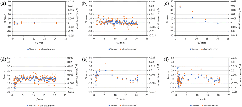
RPO methods were found to have little error (average % error for RPO step change = 2.5% Fig. 10b, and for RPO ramp = 3.5% Fig. 10d), although the error at the beginning of the RPO ramp is greater than expected. Notably, this demonstrates lower average percentage error for the RPO step change compared to the RPO ramp in this case. Interestingly, the error is negative, suggesting a lower residence time early on in the experiment than expected (Fig. 10d). However, once again the PO full step method (Fig. 10c) has significant error with both % error (blue dots) and absolute error (orange triangles, average % error = 12.9%) decreasing as the residence time increases. This suggests lower error at the beginning of the experiment (longer residence times) and increasingly greater error as the experiment progresses, presumably as the later data has experienced a greater time in the reactor at a flow rate which was below the expected value. Small PO step changes (0.2–1 mL min−1 and 1–5 mL min−1) show relatively little error compared to the full PO step change, although they deviate slightly more than the RPO step change data (Fig. 10b) and produce more sparse data. Error in the PO methods once again tends toward greater conversions, representing longer residence times than expected in all cases.
In this example, a longer 15 minute PO ramp (Fig. 10f) was also compared, which appears to have less deviation from steady state data, although this data is still relatively noisy. PO ramp data for both the 5 minute (Fig. 10e, average % error = 7.1%) and 15 minute ramps (Fig. 10f, average % error = 5.8%) show good low error at the beginning of the experiment (longer residence times) and then increase in error during intermediary residence times, before decreasing again towards the final steady state. The slower ramp rate may mitigate deviations from the steady state data by increasing flow rate at a rate at which the pumps can accurately change. If the pump rate of change is the key factor in the observed deviations of PO experiments, this could potentially be mitigated by using syringe pumps as these have a smoother transition in flow rate, although syringe pumps have other limitations such as lower maximum working pressures and limited volumes.
Aromatic Claisen rearrangement
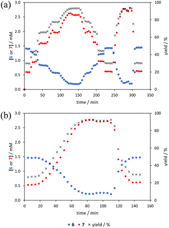
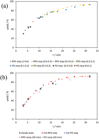
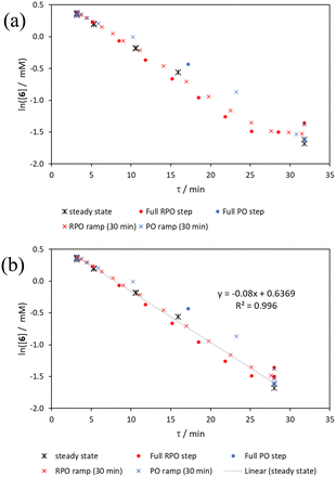
The comparison of methods for the aromatic Claisen rearrangement reaction was performed across two experiments (Fig. 11). In both experiments on-line HPLC analysis afforded quantification of the starting phenyl ether 6 concentration (blue dots) and the product phenol 7 concentration (red dots), and subsequently yield (grey crosses), through comparison of peak areas for 6 and 7 with the area of the internal standard peak. In the first experiment (Fig. 11a), small RPO and PO step changes (Fig. 12a, coloured diamonds and squares, respectively) were performed, followed by full RPO and PO step changes between 0.1–1 mL min−1 (Fig. 12b, red and blue dots, respectively) to capture the time course of the reaction. In the second experiment (Fig. 11b), a RPO linear flow rate ramp (1–0.1 mL min−1 over a 30 min ramp) followed by a PO linear flow rate ramp (0.1–1 mL min−1 over a 30 min ramp) were performed (Fig. 12b, red and blue crosses, respectively).The pseudo-first order behaviour of this reaction allowed data linearisation via a natural logarithm of the starting material (6) concentration to better compare error between methods (Fig. 13a). On performing this linearisation, it becomes apparent from the denser RPO methods (red dots and crosses) that there is an asymptote in the data after a residence time of 28 minutes at circa. 92% yield, potentially due to product auto inhibition or unseen side reactions at high conversions. It is noteworthy that this asymptotic behaviour is not readily observable from the less data dense methods such as the full PO step change (blue dots), PO ramp (blue crosses), or steady state data points (black asterisks). This discrepancy from pseudo-first order behaviour unfortunately makes method comparison by fitting a straight line to linearised steady state data points invalid. Further options for method comparison were curve fitting an arbitrary polynomial to the (low density) steady state data points (as utilised for the Knorr pyrazole synthesis example for an unknown kinetic rate law) or moving any data points at longer residence time than the asymptote time (28 min) to the asymptote time. The second option (Fig. 13b) was selected in this case to avoid inclusion of any potentially erroneous RPO data in the fitting.
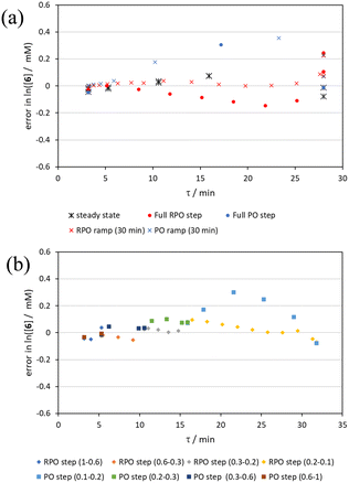
By the linearisation of this modified data, the error in the different methods can now be compared (Fig. 14), revealing, once again, greater discrepancy from PO methods (blue dots and crosses, and coloured squares). These data demonstrate that data collected via RPO methods are more accurate in all cases than those from PO methods, and that the best quality data can be obtained from RPO ramps (Fig. 14a, red crosses) or small RPO step changes (Fig. 14b, coloured diamonds), although the full RPO step (Fig. 14a, red dots) still produces relatively accurate data. Average error magnitude in the natural logarithm of concentration values of each method are ε = 0.09 (RPO step, red dots), 0.12 (PO step, blue dots), 0.04 (RPO ramp, red crosses), and 0.10 (PO ramp, blue crosses).
These data show that PO methods always under predict conversion (positive error in natural logarithm of starting material concentration), while RPO methods slightly over predict conversion. This contrasts with the previous examples in which the reaction progress was found to be over predicted for PO experiments. The inverse occurring in this case could be caused by the more extreme reaction temperature (220 °C). At faster flow rates there will be a greater length of reactor which takes longer to accurately reach the reaction temperature. This would cause PO methods – in which the reaction data is primarily collected at faster flow rates – to have a shorter reactor length at the reaction temperature and thus produce results with depressed reaction progress. This is a system limitation which could occur in any system independent of heating method when high flow rates and high temperatures are required, thus requiring greater heat flux. The effect of this insufficient heat flux is less pronounced in RPO methods due to the greater time spent at lower flow rates in which sufficient heating power can be applied.
Conclusions
‘Push out’ and ‘reverse push out’ cumulative flow rate step change and ramping methods were compared using three exemplar reactions of varying complexity: the hydrolysis of acetic anhydride, the Knorr pyrazole synthesis, and the aromatic Claisen rearrangement. Through direct comparison of data obtained from the different methods, and quantitative error analysis, all the examples demonstrated that RPO methods produce more accurate data than PO methods. These results suggest that previous work demonstrating errors from step changes can be primarily attributed to the direction of the step change, and therefore that RPO step changes are a useful simple method for collecting kinetic data from a reaction in flow.14,15 This method produced high quality kinetic data utilising a simple method with programmable single piston HPLC pumps. As the simple RPO step change can be performed manually, this could be achieved with other manually controlled or programmable pumps, and although utilisation of different types of pump may affect the error in the data obtained, the trends should remain similar.Development of an improved mathematical method for deconvoluting residence times from linear flow rate ramps allows more reaction data to be obtained from these ramps and in systems containing dead volumes. Utilising linear flow rate ramps it was demonstrated that RPO ramps were also more accurate than their equivalent PO ramps, although by ramping at a slow enough ramp discrepancies could be mitigated. This demonstrates that the standard use of RPO type linear flow rate ramps, and related linear residence time ramps, is justified in comparison to PO ramps. These linear flow rate ramps, however, require programmable pumps, although pumps with the capability of performing linear flow rate ramps are more available and cheaper than those for more complex flow rate ramps, such as those used to produce linear residence time ramps.
Comparing RPO step changes to RPO ramps demonstrated similar data accuracy and data density in the discussed examples. In light of this work, RPO step changes should be considered the preferred method for those new to the field for reaction time series data collection in transient flow experimentation, due to the simpler implementation and deconvolution of these methods. For those researchers in industry and academia interested in collecting accurate kinetic data a RPO step change should be a quick and easy first port of call, possible with almost all flow setups in either a manual or automated fashion. Of course, in exceptional cases in which residence times are small in comparison to analytical speed, or if greater experimental complexity is not prohibitive, a slower ramp should be used to increase data density. Other than these cases, the RPO step method offers comparable data accuracy while requiring simpler deconvolutional methods, cheaper less sophisticated equipment, less experimental time, and less material than a ramping method.
Author contributions
LS conducted the experimental work, collected and analysed the data. All other authors offered advice during the work and mentorship to LS. LS and KKH wrote the original draft and subsequent revisions of the manuscript, which were reviewed by all the other authors.Conflicts of interest
There are no conflicts to declare.Acknowledgements
We are grateful to BASF SE and the EPSRC REACT CDT [EP/S023232/1] for financial support. This project was supported by access to instrumentation and expertise at the Centre for Rapid Online Analysis of Reactions (ROAR) at Imperial College London [EPSRC, EP/R008825/1 and EP/V029037/1]. We are grateful to Imperial College Advanced Hackspace for their help in constructing the Peltier cooling device.References
- M. Rodriguez-Zubiri and F. O.-X. Felpin, Org. Process Res. Dev., 2022, 26, 1766–1793 CrossRef CAS.
- S. V. Ley, D. E. Fitzpatrick, R. J. Ingham and R. M. Myers, Angew. Chem., Int. Ed., 2015, 54, 3449–3464 CrossRef CAS PubMed.
- A. Gioiello, A. Piccinno, A. M. Lozza and B. Cerra, J. Med. Chem., 2020, 63, 6624–6647 CrossRef CAS PubMed.
- C. J. Taylor, J. A. Manson, G. Clemens, B. A. Taylor, T. W. Chamberlain and R. A. Bourne, React. Chem. Eng., 2022, 7, 1037–1046 RSC.
- D. E. Fitzpatrick, T. Maujean, A. C. Evans and S. V. Ley, Angew. Chem., Int. Ed., 2018, 57, 15128–15132 CrossRef CAS PubMed.
- C. P. Haas, M. Lübbesmeyer, E. H. Jin, M. A. McDonald, B. A. Koscher, N. Guimond, L. Di Rocco, H. Kayser, S. Leweke, S. Niedenführ, R. Nicholls, E. Greeves, D. M. Barber, J. Hillenbrand, G. Volpin and K. F. Jensen, ACS Cent. Sci., 2023, 9, 307–317 CrossRef CAS PubMed.
- L. Schrecker, J. Dickhaut, C. Holtze, P. Staehle, M. Vranceanu, K. Hellgardt and K. K. Hii, React. Chem. Eng., 2023, 8, 41–46 RSC.
- L. Schrecker, J. Dickhaut, C. Holtze, P. Staehle, A. Wieja, K. Hellgardt and K. K. Hii, React. Chem. Eng., 2023, 8, 3196–3202 RSC.
- J. Van Herck and T. Junkers, Chem.: Methods, 2022, 2, e202100090 CAS.
- C. J. Taylor, M. Booth, J. A. Manson, M. J. Willis, G. Clemens, B. A. Taylor, T. W. Chamberlain and R. A. Bourne, Chem. Eng. J., 2021, 413, 127017 CrossRef CAS.
- F. E. Valera, M. Quaranta, A. Moran, J. Blacker, A. Armstrong, J. T. Cabral and D. G. Blackmond, Angew. Chem., Int. Ed., 2010, 49, 2478–2485 CrossRef CAS PubMed.
- M. V. Gomez, A. M. Rodriguez, A. De La Hoz, F. Jimenez-Marquez, R. M. Fratila, P. A. Barneveld and A. H. Velders, Anal. Chem., 2015, 87, 10547–10555 CrossRef CAS PubMed.
- D. P. Rütti, M. Moser, A. G. Georg, E. S. Spier and D. M. Meier, Chem. Ing. Tech., 2021, 93, 1267–1272 CrossRef.
- S. Mozharov, A. Nordon, D. Littlejohn, C. Wiles, P. Watts, P. Dallin and J. M. Girkin, J. Am. Chem. Soc., 2011, 133, 3601–3608 CrossRef CAS PubMed.
- T. Durand, C. Henry, D. Bolien, D. C. Harrowven, S. Bloodworth, X. Franck and R. J. Whitby, React. Chem. Eng., 2016, 1, 82–89 RSC.
- C. A. Hone, N. Holmes, G. R. Akien, R. A. Bourne and F. L. Muller, React. Chem. Eng., 2017, 2, 103–108 RSC.
- J. S. Moore and K. F. Jensen, Angew. Chem., Int. Ed., 2014, 53, 470–473 CrossRef CAS PubMed.
- X. Duan, J. Tu, A. R. Teixeira, L. Sang, K. F. Jensen and J. Zhang, React. Chem. Eng., 2020, 5, 1751–1758 RSC.
- F. Florit, A. M. K. Nambiar, C. P. Breen, T. F. Jamison and K. F. Jensen, React. Chem. Eng., 2021, 6, 2306–2314 RSC.
- S. P. Asprey, B. W. Wojciechowski, N. M. Rice and A. Dorcas, Chem. Eng. Sci., 1996, 51, 4681–4692 CrossRef CAS.
- A. Zogg, F. Stoessel, U. Fischer and K. Hungerbühler, Thermochim. Acta, 2004, 419, 1–17 CrossRef CAS.
- A. Ładosz, C. Kuhnle and K. F. Jensen, React. Chem. Eng., 2020, 5, 2115–2122 RSC.
- D. P. N. Satchell, W. N. Wassef and Z. A. Bhatti, J. Chem. Soc., Perkin Trans. 2, 1993, 2, 2373–2379 RSC.
- C. A. Bunton, N. A. Fuller, S. G. Perry and V. J. Shiner, J. Chem. Soc., 1963, 44, 3028–3036 Search PubMed.
- W. N. White, D. Gwynn, R. Schlitt, C. Girard and W. Fife, J. Am. Chem. Soc., 1958, 80, 3271–3277 CrossRef CAS.
- H. Kobayashi, B. Driessen, D. J. G. P. Van Osch, A. Talla, S. Ookawara, T. Noël and V. Hessel, Tetrahedron, 2013, 69, 2885–2890 CrossRef CAS.
Footnote |
| † Electronic supplementary information (ESI) available. See DOI: https://doi.org/10.1039/d3re00696d |
| This journal is © The Royal Society of Chemistry 2024 |

