Development of a surrogate artificial neural network for microkinetic modeling: case study with methanol synthesis

Abstract

Microkinetic models allow the description of complex reaction kinetics but require high computational costs, hindering their combination with detailed reactor models. In this contribution, a methodology to develop a surrogate artificial neural network (ANN) was proposed and demonstrated for methanol synthesis on Cu/Zn-based catalysts. The resulting model accurately reproduces the simulations of the original microkinetic model, reducing the computational costs by orders of magnitude. In the developed methodology, the ANN learns only the kinetics of the global reaction rates, thereby decreasing model complexity and computational costs while ensuring thermodynamic consistency. In addition, an improved activation function for the ANN was designed in this work to minimize computational costs and to smooth out calculations. The proposed approach creates a bridge to integrate microkinetics into applications in the field of reaction engineering, such as reactor design, process optimization, and scale-up.

---

1. Introduction

Microkinetic modeling is the mathematical representation of global reactions (e.g. CH₃OH formation from CO and H₂) considering elementary steps (e.g. H₂ adsorption to H*) of a typically complex reaction network. This type of modeling has been significantly enhanced over the past years.¹ It has been supported by advances in quantum chemical calculations^2,3 and by improvements in the quality of kinetic experiments (e.g. better analytics, improved automation, better process monitoring and control) as well as in the possibility of faster generation of high amounts of data (e.g. by high-throughput experimentation).⁴

However, due to the high computational costs of microkinetic models (MKMs), their application in combination with detailed reactor models is hindered. A promising alternative is the development of surrogate models that are able to learn the behavior of the microkinetic model and reproduce its simulations at much lower computational costs.¹

Spline functions have been proposed to fulfill this purpose and have shown accurate results for a variety of reaction systems but have high storage requirements that scale exponentially with the number of inputs.^5–7 To overcome these storage limitations, the application of an in situ adaptive tabulation technique was shown to be successful.^8,9

As an alternative to spline interpolation, machine-learning techniques have been investigated for the development of surrogate models of microkinetics.^10–12 In comparison with spline functions, it has been demonstrated that artificial neural networks (ANNs) had much lower computational costs and storage requirements, while higher accuracy was achieved with a smaller training database.¹²

For reaction rates of a given system that span several orders of magnitude, model accuracy was improved by using the logarithmic function of the reaction rates and concentrations and the inverse of temperature.^5,10 As the logarithmic function requires strictly positive inputs, a question arises on how to deal with reaction rates that are sometimes positive and sometimes negative. Therefore, Partopour et al.¹¹ proposed to separately learn the adsorption and desorption of each participating species. Recently, Döppel and Votsmeier¹² proposed to map out the rate-determining steps and learn the forward and the reverse reactions separately.

In this contribution, a comprehensive methodology is presented to transfer information from a microkinetic model MKM to an ANN, maintaining model accuracy while sharply decreasing computational costs. The kinetics and thermodynamics of the global reaction rates are split, so that the former are learned by the ANN, while the latter are calculated afterward by known equations. This approach has two direct benefits: the kinetics are strictly positive (addressing the question posed in the last paragraph), and the thermodynamic consistency of the model is ensured. In addition, a new activation function for the ANN is proposed here, which was designed to minimize computational costs. To demonstrate this methodology, our recently published microkinetic model of the methanol synthesis on Cu/Zn-based catalysts¹³ was taken as a case study.

2. Methodology

2.1 Microkinetic model (MKM) description

The microkinetic model considered in this work¹³ is based on density functional theory (DFT).^14,15 It describes the methanol synthesis on Cu/Zn-based catalysts, with reactants and products in the gas phase, and intermediates adsorbed on the catalyst surface. In this model, all three main global reactions involved in the methanol synthesis were considered: CO hydrogenation (eqn (1)), CO₂ hydrogenation (eqn (2)), and the water-gas shift reaction (WGSR, eqn (3)). The reaction network is shown in Fig. 1.

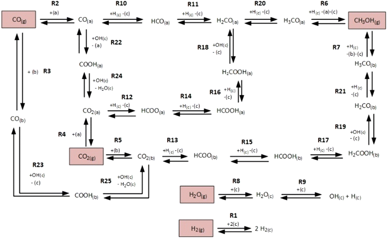Fig. 1 Reaction network of the microkinetic model. Adapted with permission from Campos et al.¹³ Copyright 2021 Royal Society of Chemistry.

In this model, three different active sites were considered: site (a) (pure Cu), site (b) (Cu/Zn), and site (c) (Cu or Cu/Zn available only for H₂ and H₂O adsorption). Assuming a mean-field approximation, the rate of a reversible elementary step k (r_k, in mol kg_cat⁻¹ s⁻¹) was calculated following the Eyring–Polanyi equation.^16,17 This rate equation can be split into intrinsic kinetics (i.e. reaction constant k), gas phase dependency (F_G), and catalytic surface dependency (F_C).

The reaction constant (k) was calculated as follows:

Here, T is the reaction temperature (K), β_k is a correction term to ensure thermodynamic consistency,^13,18k_b is the Boltzmann constant (kJ K⁻¹), h is the Planck constant (kJ s), E_A,k is the activation energy (kJ mol⁻¹), ΔS^≠_k is the entropy barrier (kJ mol⁻¹ K⁻¹), and R is the universal gas constant (kJ mol⁻¹ K⁻¹).

The gas phase and catalyst surface dependencies were calculated with the following expressions:

where N_G is the number of gas phase components, N_S is the number of surface intermediates, f_j is the fugacity of gas component j (bar), p₀ is the reference pressure (bar), n_M,Cat is the number of active sites per catalyst mass unit (mol kg_cat⁻¹), ϕ_i is the fraction of the site type of surface species i in relation to the total number of sites for carbon-containing compounds (sites a and b), θ_i is the surface coverage of intermediate i, is the stoichiometric coefficient of species i in the forward direction of reaction k, and is the stoichiometric coefficient of species i in the reverse direction of reaction k.

Finally, the rate of a reversible reaction k is given by combining eqn (4)–(6).

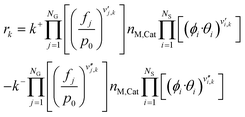
r_k = k⁺·F⁺_G·F⁺_C − k⁻·F⁻_G·F⁻_C (7)

Here, the superscripts + and − refer to the forward and reverse reactions, respectively.

The surface coverages were obtained with balance equations, resulting in a system of ordinary differential equations (eqn (9)).

In general, the time needed for the reactive surface to reach a steady-state after a perturbation is orders of magnitude lower than the time needed for the reactor to stabilize after a change in the process conditions.²³ Because of that, the steady-state solution of the kinetic model (eqn (9) with dθ_i/dt = 0) should be useful to simulate reactors in both steady-state and transient conditions. There are two ways to find the steady-state solution of eqn (9):

• To integrate the equations in time until steady state is achieved. MATLAB function ode23s was chosen to solve this stiff system.

• To make dθ_i/dt = 0, deriving a non-linear algebraic system of equations, which can be solved, e.g. with MATLAB function fsolve.

The second option has lower computational costs than the first one, but it requires educated initial values to converge to the correct solution. If these values are not known, then the time integration should be performed. In this work, the time integration from 0 to 15 s was performed, which was sufficient to reach steady state in all cases. The initial condition for the time integration was chosen case-by-case based on an initial guess method developed in a previous work (see Fig. S1 in the ESI†).¹³ With these educated guesses, a typical integration time to reach steady state was 1.5 s, while random initial conditions took longer but reached the same results (e.g. if all coverages were set to 0.01 as the initial condition, a typical time to reach steady state was 8 s).

Independently if the time integration or the algebraic system resolution is chosen, it is highly recommended to provide the analytical Jacobian matrix, as computational costs are significantly lowered and numerical instability is avoided. In addition, the analytical derivation of the Jacobian matrix for this type of mathematical system is relatively easy due to the nature of the equations (either linear or quadratic dependency on the variables).

The rates of the global reactions (eqn (1)–(3)) are equal to the rate of the following elementary steps (see Fig. 1):

r_CO = r₁₀ (10)

r_CO2 = r₁₄ + r₁₅ (11)

r_WGS = r₂₂ + r₂₃ (12)

The kinetic parameters (E_A,k, ΔS^≠_k) were taken from DFT calculations,^14,15 and only n_M,Cat was fitted to experimental data. A total of 690 steady-state experiments from different setups^13,24–26 were used to validate this model at a wide range of operating conditions. The kinetic parameters (E_A,k, ΔS^≠_k) and the correction terms (β_k) are provided in the ESI,† section S1.

2.2 Inputs of the artificial neural network (ANN)

To minimize the complexity and computational costs of the ANN, the number of inputs should be as low as possible. Still, the given inputs should sufficiently describe the reaction conditions (i.e. the number of inputs should be as high as necessary).

In our case study, the microkinetic model of the methanol synthesis requires six inputs to calculate the reaction rate of a certain reaction condition: temperature (T) and the fugacity of each gas species participating in the reactions (f_H2, f_CO, f_CO2, f_CH3OH, f_H2O). Therefore, these same inputs are considered for the ANN. Note here that the total pressure (p) must not be explicitly given as an extra input because the effect of non-ideality is already contained within the fugacities. Besides, the fugacity of (possible) inerts is only necessary in the reactor model and must not be given as extra inputs in the reaction model.

2.3 Outputs of the artificial neural network (ANN)

A microkinetic model generally provides the following outputs: the coverage of the surface species, the rate of the elementary steps, and the rate of the global reactions. In this work, the focus is on the rate of global reactions (in this case study: r_COr_CO2, r_WGS), which is normally the most interesting information for the reactor model. Nonetheless, the methodology described here is most likely to work for the other outputs as well.

It is known that the rate of a global reversible reaction consists in a kinetic part (r^K) and a thermodynamic part (r^T), which are multiplying each other. This is explicit in formal kinetic models, exemplified here for CO₂ hydrogenation to methanol:²⁷

r = [Kin. term]·(Therm. term) = r^K·r^T (13)

where A₂ and E_A,2 (kJ mol⁻¹) are kinetic parameters and (bar⁻²) is the global equilibrium constant of the CO₂ hydrogenation to methanol.

In microkinetic models, it is possible to isolate the kinetic and thermodynamic terms if there is a single global reaction (see the mathematical demonstration in the ESI,† section S2). For multiple global reactions, which is the case for the majority of the systems, the kinetic term of global reaction n (r^K_n) can be indirectly obtained by dividing the reaction rate (r_n) by the thermodynamic term (r^T_n):

where N_P is the number of products, N_R is the number of reactants, is the stoichiometric coefficient of species i in the forward direction of global reaction n, and is the stoichiometric coefficient of species i in the reverse direction of global reaction n.

The kinetic term is the most complex part of the reaction rate estimation. It is the subject of thorough theoretical and experimental investigations, and, therefore, the reason for a variety of kinetic models in the literature describing the same system. In contrast, the thermodynamic term of a global reaction, often called “the affinity of the reaction towards the equilibrium”,²⁸ can be easily calculated with fugacities and global equilibrium constants, which are generally described by known thermodynamic equations.

Therefore, the ANN should be used to learn and predict only the complex part (i.e. the kinetics, r^K), while the thermodynamics (r^T) can be calculated afterward with simple known equations (eqn (18)). The application of this procedure brings three benefits:

• A priori information is being used, reducing the amount of information the ANN has to learn and, therefore, its complexity.

• The thermodynamic consistency of the model is ensured.

• The kinetic terms (r^K) are strictly positive, giving a suitable solution to the issue discussed in the introduction, i.e. manipulating the reaction rates with the logarithmic function, which requires strictly positive values.

Hence, it makes sense to set the outputs of the ANN to be r^K_n instead of r_n. In this case study, the outputs of the ANN are then r^K_CO, , and r^K_WGSR. For the methanol synthesis, the thermodynamic terms and the equilibrium constants are given as follows:^13,27,29

K⁰_P,CO = T^−3.384·exp(10 092.4T⁻¹ − 4.200) (22)

K⁰_P,WGS = T^1.097·exp(5337.4T⁻¹ − 12.569) (24)

In Fig. 2, the pathways from inputs to outputs for both the MKM and the ANN are illustrated.

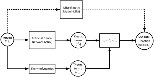Fig. 2 Pathway from inputs to outputs for the microkinetic model (MKM) (dashed lines) and the proposed artificial neural network (ANN) (solid lines).

2.4 Data generation with the microkinetic model

In order to train the ANN, data must be provided, which is to be generated by the validated microkinetic model. The data should be selected in a way that the ANN is sensitive to all input parameters at the desired operating window. The most straightforward and simple way would be to spread data points evenly across a relevant space regarding the inputs (temperature and fugacities). In our case, to avoid generating data in a region of methanol consumption far away from the equilibrium (a region in which the microkinetic model itself was not validated experimentally), an alternative methodology was applied, which is explained as follows.

The microkinetic model was coupled with a reactor model of a plug flow reactor (PFR), considering variations only along the reactor length (1D model) and assuming isobaric and isothermal conditions. These considerations resulted in the following balance equations along the reactor length:

where ṅ is the total mole flow (mol s⁻¹), z is the axial direction (m), m_cat is the total catalyst mass in the catalyst bed (kg), L is the catalyst bed length (m), y_j is the mole fraction of gas component j, is the stoichiometric coefficient of species i in the forward direction of global reaction n, and is the stoichiometric coefficient of species i in the reverse direction of global reaction n.

To model the real gas behavior and calculate the fugacities, the Peng–Robinson equation of state was used.¹⁹ Binary interaction parameters (k_ij) and other necessary data reported in the literature are considered,^20,21 and an effective hydrogen acentric factor of ω = −0.05 was assumed.²²

For a certain operating condition, first the equilibrium H₂ conversion (X_H2,eq.) was calculated (the methodology is provided in the ESI,† section S2). Then, the operation of a long PFR was simulated in MATLAB (integration with the function ode45), with the hydrogen conversion (X_H2) being calculated in each step (eqn (21)), and an event function to stop the integration if the system is close to chemical equilibrium (eqn (22)).

Stop integration if: X_H2 ≥ 0.95·X_H2,eq. (28)

Here, X_H2 is the H₂ conversion, ṅ_H2 is the hydrogen mole flow (mol s⁻¹), while the subscripts indicate the axial position.

Finally, data points were collected from the PFR simulation at different X_H2/X_H2,eq values, totalizing 21 points for each simulation. The differential equations (eqn (19) and (20)) were solved in MATLAB with the function ode45, with relative and absolute tolerances set to 10⁻⁸. In Table 1, the chosen operating conditions are summarized, amounting to a total of 5720 simulations and 120 120 data points.

Table 1 Operating conditions of the data generation with the microkinetic model

Parameter	Values	No. of conditions
Simulation conditions
Pressure (bar)	20, 25, 30, 35, 40, 45, 50, 55, 60, 65, 70	11
Temperature (K)	483.15, 488.15, 493.15, 498.15, 503.15, 508.15, 513.15, 518.15, 523.15, 528.15, 533.15, 538.15, 543.15	13
H2/COX in feed	0.67, 1.00, 1.50, 2.33, 4.00	5
CO2/COX in feed	0.02, 0.08, 0.15, 0.22, 0.29, 0.36, 0.43, 0.50	8
Total number of simulations		5720
Data point collection in each simulation
X H2/XH2,eq	0.00, 0.025, 0.05, 0.10, 0.15, 0.20, 0.25, 0.30, 0.35, 0.40, 0.45, 0.50, 0.55, 0.60, 0.65, 0.70, 0.75, 0.80, 0.85, 0.90, 0.95	21
Total number of data points		120 120

---

CO₂/CO_X in feed between 0.02 and 0.50 were chosen, because this is the region where this microkinetic model excels.¹³ The feed mole fractions of H₂, CO, and CO₂ (respectively , yⁱⁿ_CO, and ) were defined as follows:

The information saved in each data point are the six inputs (T, f_H2, f_CO, f_CO2, f_CH3OH, f_H2O) and the reaction rates (r_CO, r_CO2, r_WGS). Since the microkinetic model does not explicitly calculate the kinetic part of the reaction rates (r^K_n), this was calculated separately:

After this last calculation (eqn (26)–(28)), each data point contains the necessary information to train the ANN: six inputs (T, f_H2, f_CO, f_CO2, f_CH3OH, f_H2O) and three outputs (r^K_CO, , r^K_WGS).

2.5 Artificial neural network structure

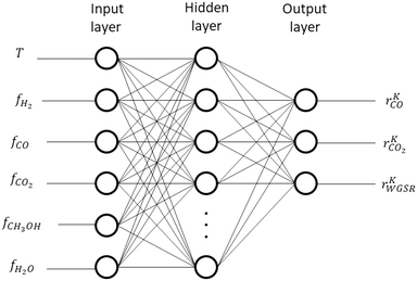
The chosen structure of the ANN consists of one input layer (IL) with six cells (corresponding to the number of inputs), one hidden layer (HL), and one output layer (OL) with three cells (corresponding to the number of outputs). ANNs with different number of cells in the hidden layer were developed, and the results were compared and discussed. The number of hidden layers was kept to one because good results were shown in the literature for related systems,¹² and adding further layers would significantly increase model complexity and computational time.

As mentioned in the introduction, the usage of the logarithmic function for both the reaction rates and the component concentrations is beneficial if the reaction rates span over several orders of magnitude.^5,10 As it was not the case for the present system, this approach was not followed in this case study. Instead, a normalization of input j in each cell j of the input layer (IL) was performed:

Here, I_j is the original value of input j, I_j,min is the minimum value of input j, I_max is the maximum value of input j, and I_j,norm, is the normalized value of input j. The minimum and maximum allowed values for each input are given in Table 2, which correspond to the operating window of Table 1 with a slight extension (5–10%).

Table 2 Minimum and maximum allowed values of the inputs and outputs of the ANN

Variable	Minimum	Maximum	Unit
Inputs
T	483.15	553.15	K
f H2	0	60	bar
f CO	0	50	bar
f CO2	0	30	bar
f CH3OH	0	30	bar
f H2O	0	5	bar
Outputs
r ^KCO	0	180	mol kgcat^−1 h^−1
	0	240	mol kgcat^−1 h^−1
r ^KWGSR	0	450	mol kgcat^−1 h^−1

---

In the hidden layer (HL), two mathematical operations occur in series in each cell w: first an aggregation function, then an activation function. Typically, the aggregation function is a sum of weighted inputs, which was also the approach considered here:

where s_w,in is the input value to cell w, p_wj is a model parameter of cell w and input j, p_w0 is a model parameter of cell w (independent term), and N_I is the number of ANN inputs.

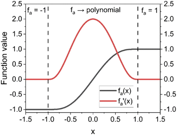
Generally, activation functions, named here f_a(x), are selected to give non-linearity to the model and to saturate at high absolute values of x (i.e. f_a tends to a constant value for high x on both positive and negative directions). Typical non-linear activation functions are the hyperbolic tangent (tanh) and the sigmoid function.

Our interest was that the activation function and its first derivative are continuous in the whole x domain, thereby smoothing out calculations. Finally, the main goal of this work was to minimize computational costs, which should be remembered when choosing or designing an activation function.

Considering these characteristics, a new activation function was developed in this work, which has not been proposed elsewhere, to the best of our knowledge. The function, presented in Table 3, has three regions: constant f_a = 1 for x ≥ 1 , constant f_a = −1 for x ≤ −1, and a ninth-degree polynomial for −1 < x < 1. The polynomial was designed to be an odd function, i.e. f(−x) = −f(x), and to provide a smooth transition between the three different regions, so that the activation function and its first derivative are continuous along the complete real domain. The continuity and smoothness of f_a(x) and can be seen in Fig. 3.

Table 3 Activation function proposed in this work (f_a) and its first derivative

x	f a(x) and
x ≤ −1	f a(x) = −1
−1 < x < 1	f a(x) = x·{2 + x^2 ·[−1.4375 + x^2·(0.1875 + x^2·(0.4375 – 0.1875·x^2))]}
x ≥ 1	f a(x) = 1

---

Fig. 3 Activation function proposed in this work [f_a(x)] and its first derivative .

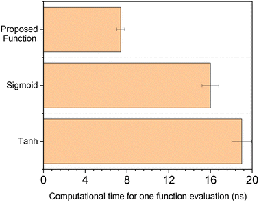
The computational time of the proposed function was compared to that of typical activation functions used in the literature for this field.^12,30 The methodology was to evaluate the function for a random input 10⁸ times in the range |x| ≤ 1.2. Both the sigmoid and the hyperbolic tangent were written using MATLAB function exp(x), instead of directly calling built-in functions tanh(x) or sigmoid(x), which are slower. Calculation time was given by MATLAB function tic toc, and the procedure was performed ten times to obtain average values and confidence intervals. All calculations were performed in MATLAB 2018a with the same computer (processor: Intel Core i7-7700 CPU @ 3.60 GHz, installed RAM: 32 GB, operating system: Windows 10 64 bit).

In Fig. 4, the computational time of the different functions is displayed. Our proposed function is more than two times faster than the hyperbolic tangent and the sigmoid function. Similar results were obtained by lowering the range of x to |x| ≤ 1, increasing it to |x| ≤ 2 or even to |x| ≤ 10.

Fig. 4 Average computational time of one function evaluation for different activation functions.

The computational costs of the developed activation function are significantly lower due to the following characteristics:

• In contrast to highly non-linear functions which must be calculated iteratively (e.g. sin(x), e^x), a polynomial is analytically calculated with simple operations (i.e. addition, subtraction and multiplication), requiring much lower computational costs.

• The polynomial was written in a way that minimizes the number of mathematical operations to only 10. This alternative description also avoids roundoff errors caused by finite-precision rounded arithmetic, which could appear in a typical polynomial calculation when adding up terms with large differences in the exponential factor.

• When the function is in the saturation region (|x| ≥ 1), the polynomial evaluation is not necessary, leading to minimal computational costs. This is another advantage of our activation function in relation to equations that tend to a constant value, such as tanh(x) and sigmoid(x), but still needs to be calculated in the whole function domain.

The output value of each cell w of the HL (s_w,out) is the outcome of the activation function:

s_w,out = f_a(s_w,in) (37)

In the output layer (OL), the aggregation function (eqn (38)) and the activation function (eqn (39)) are also present:

ŝ_w,out = f_a(ŝ_w,in) (39)

where ŝ_w,in is the input value of cell n, ŝ_n,out is the output value of cell n, N_HL is the number of cells of the HL, p_nw is a model parameter of cell w and output n, and p̂_0w is a model parameter of cell w (independent term).

With the output values of the activation function (ŝ_n,out), the kinetic part of the reaction rates (r^K_k) were then obtained:

r^K_n = 0.5·r^K_n,max·(ŝ_n,out + 1) (40)

Here, r^K_n,max is the maximum value allowed for r^K_n. The maximum allowed values of the outputs were set to values moderately higher than the operating window covered by the generated data, and they are summarized in Table 2. The structure of the ANN is illustrated in Fig. 5.

Fig. 5 ANN structure.

Finally, to obtain the reaction rates, the kinetic term of global reaction n (eqn (40)) and the corresponding thermodynamic term (eqn (19)–(21)) are multiplied, as already shown in Fig. 2.

r_n = r^K_n·r^T_n (41)

2.6 Artificial neural network training

The ANN with the structure described in section 2.4 has two matrices of parameters to be optimized:

• One for the hidden layer (p_wj, eqn (36)), with N_HL × N_I elements

• One for the output layer (p̂_nw, eqn (38)), with N_HL × N_O elementswhere N_HL is the number of cells in the hidden layer, and N_O is the number of outputs.

In order to estimate these parameters, the data points generated with the MKM (120 120 points) were randomly divided between training (80%), test (10%) and validation (10%). The training points were used to solve the optimization problem, whose goal was to minimize the deviations between the MKM and the ANN predictions of the r^K_n:

Here, N_GR is the number of global reactions, N_TP is the number of training points, w_ni are selected weights, and the subscripts MKM and ANN refer to simulations performed by the microkinetic model and the artificial neural network, respectively.

As the main interest is the prediction of the reaction rates (r_n), the weights chosen were the thermodynamic term of the reaction rates (r^T_n), reducing the influence of points close to the equilibrium. While r^T_n is limited to +1 in the positive direction, it is unlimited in the negative direction. Therefore, a limit of 10 was set to w_ni:

w_ni = |r^T_ni| (43)

if w_ni > 10, then w_ni = 10 (44)

In this work, ANNs with 10, 20, 30, and 40 cells in the hidden layer (N_HL) were trained. They are named here ANN₁₀, ANN₂₀, ANN₃₀, and ANN₄₀, respectively. First, ANN₁₀ was trained with random initial guesses. The parameters of the optimized ANN₁₀ were used as initial guesses to train ANN₂₀, with the new additional parameters (present only in ANN₂₀) receiving random initial guesses with low absolute values. The same procedure was applied when training ANN₃₀ and ANN₄₀.

To solve this minimization problem, the quasi-Newton method was applied. To find the search direction, the gradient of the objective function was analytically calculated, and the inverse of the Hessian matrix was iteratively updated with the Broyden–Fletcher–Goldfarb–Shanno (BFGS) algorithm. After the search direction was defined, the optimal step size was determined by line search. The optimization problem was written and solved in C language.

2.7 Coupling the ANN with reactor models

The ANN can be easily coupled with different reactor models, the same way as a formal kinetic model or a microkinetic model. As a final validation step in this work, the ANN was coupled to reactor models in order to reproduce real laboratory data.

For the plug flow reactor (PFR), the same procedure described in section 2.4 is made (eqn (23) and (24)), the only (obvious) difference being that r_CO, r_CO2, and r_WGS were calculated by the ANN instead.

For the continuous stirred tank reactor (CSTR), considering steady-state operation of a gradient-free reactor, the following balance equations for each component and the total mole flow exiting the reactor (ṅ_out) were solved:

ṅ_out = ṅ_in − 2·m_Cat·(r_CO + r_CO2) (46)

To solve this algebraic system, the function fsolve from MATLAB was used. The function and step tolerances were set to 10⁻⁸, and the experimental values were used as initial guesses of the mole fractions.

2.8 Quantifying the computational costs

To compare the computational costs between the models, the reaction rates of the 120 120 points were calculated. Calculation time was given by MATLAB function tic toc, and the procedure was performed ten times to obtain average values and confidence intervals. All calculations were performed in MATLAB 2018a with the same computer (processor: Intel Core i7-7700 CPU @ 3.60 GHz, installed RAM: 32 GB, operating system: Windows 10 64 bit).

It should be noted here that the reaction rates and derivatives were written one-by-one in the programming of the microkinetic model instead of using sparse coefficient matrices and long “for” loops, which would increase computational time. Besides, the system of equations (eqn (8) and (9)) were solved by integrating the equations from 0 to 15 s.

3. Results and discussion

The ANNs were successfully trained with the generated data from the MKM. The parameters of the ANNs are provided in the ESI† (section S4). The mean error (ME), the mean squared error (MSE), and the R² of the ANN for each reaction rate n (r_n) were calculated as follows:where N_P is the total number of data points.

In Fig. 6, statistical data of the ANN performance is presented for the different hidden layer (HL) sizes investigated. All ANNs present significantly low mean deviations, with the accuracy being considerably improved by increasing the HL size. In particular, ANN₃₀ and ANN₄₀ show excellent results, with R² close to 1, MSE close to 0, and ME below 0.15 mol kg_cat⁻¹ h⁻¹ (ca. 1% of mean reaction rate values). Since the accuracy of ANN₃₀ is significantly high and close to that of ANN₄₀, while its computational costs are lower than that of ANN₄₀ due to the former's lower complexity, ANN₃₀ seems to provide the best compromise between accuracy and computational costs. Therefore, ANN₃₀ is the model chosen for further analysis and validation.

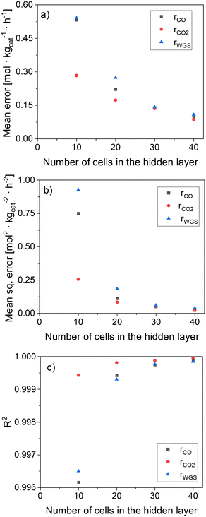Fig. 6 Statistical data of the ANN as a function of the HL size. (a) Mean error (ME). (b) Mean squared error (MSE). (c) R².

In Fig. 7, parity plots of the 120 120 reaction rate points (r_n) are shown for the ANN₃₀. The points are close to the bisector for the three global reactions, confirming that the model correctly simulates the data in the operating window studied. Besides, no significant systematic deviation was observed.

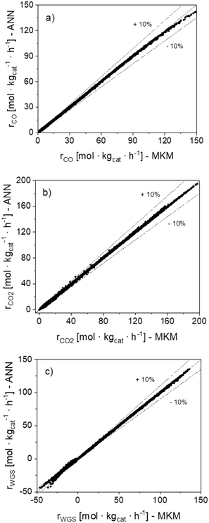Fig. 7 Parity plots of the 120 120 reaction rate points (r_n) simulated with the MKM and the ANN₃₀. (a) CO hyd. (b) CO₂ hyd. (c) WGS.

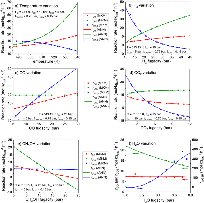
In Fig. 8, the effect of each input in the reaction rates is shown for the MKM and the ANN₃₀. The ANN₃₀ outputs are almost a perfect match to the MKM simulations, showing that the black box model correctly learned the influence of each input on the reaction rates, and no indication of overfitting is found. Some of the effects adequately learned by the ANN are, for example:

Fig. 8 Effect of each input in the rate of the global reactions simulated by the MKM and ANN₃₀. The value of each input is changed at a time, while the remaining ones are given the following constant values: T = 513.15 K, f_H2 = 25 bar, f_CO = 10 bar, f_CO2 = 5 bar, f_CH3OH = 0.75 bar, f_H2O = 0.15 bar. Variations in (a) temperature, (b) f_H2, (c) f_CO (d) f_CO2, (e) f_CH3OH, and (f) f_H2O.

• Significant temperature influence in all reactions, including a negative influence in the WGSR (as its reverse reaction is favored).

• Positive effect of H₂ fugacity in the methanol synthesis and strong negative effect of this input in the WGSR.

• Positive effect of CO fugacity on CO hydrogenation to methanol and the WGSR, while CO content does not affect CO₂ hydrogenation.

• Limited positive effect of CO₂ fugacity on CO₂ hydrogenation to methanol (as formate coverage becomes close to 100%).

• Negative effect of CO₂ fugacity on CO hydrogenation to methanol (inhibition by formate poisoning) and on the WGSR (formate inhibition and improved reverse reaction).

• Negative effect of CH₃OH fugacity on methanol synthesis (product inhibition) and no effect on the WGSR.

• Strong positive effect of H₂O fugacity on the WGSR, and negative effect on CO₂ hydrogenation to methanol (product inhibition). An inhibition of the methanol synthesis via a water intermediate (e.g. OH* or H₂O*) might probably be significant at higher water concentration, which is typical for the methanol synthesis at high CO₂ content.

The accurate reproduction of the input influence on the reaction rates is also an evidence that the ANN₃₀ can correctly predict reactor conditions at non-stoichiometric conversion. This is the case of simulations including diffusion in the mesoscale, in which the components may diffuse with different velocities and change the gas composition along the catalyst pores.

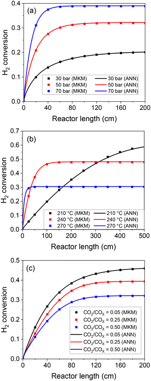
After this thorough model validation regarding the reaction rates, the ANN₃₀ was coupled with a reactor model (eqn (25) and (26)) and tested. Simulations of a plug flow reactor (PFR) at different conditions were performed by both models (ANN and MKM), and the axial profiles are presented in Fig. 9. The ANN₃₀ curves matched the MKM simulations, including correct prediction of the equilibrium. The influence of the total pressure, the temperature, and CO₂ content in both the kinetic and the thermodynamic regime was correctly described. In addition, no strange behavior is observed (e.g. oscillating behavior close to the equilibrium).

Fig. 9 Reactor simulations with the MKM and the ANN₃₀. (a) Conditions: 250 °C, 2 m³ h⁻¹ kg_cat⁻¹, feed: H₂/CO/CO₂/N₂ = 63/15/2/20% v/v. (b) Conditions: 50 bar, 0.8 m³ h⁻¹ kg_cat⁻¹, feed: H₂/CO/CO₂/N₂ = 60/20/10/10% v/v. (c) Conditions: 230 °C, 50 bar, 2 m³ h⁻¹ kg_cat⁻¹, feed: H₂/CO_X/N₂ = 70/20/10% v/v.

After all these validation steps, a final test was performed with the ANN₃₀: the simulation of real steady-state experimental data from two different setups: 234 points performed in a fixed-bed tube reactor (plug flow reactor, PFR),¹³ and 46 points performed in a Berty-type reactor (continuous stirred tank reactor, CSTR).²⁴ The operating window was wide: 30–60 bar, 210–260 °C, 3.6–40 m³ h⁻¹ kg_cat⁻¹, H₂/CO_X in feed: 0.6–5.0, CO₂/CO_X in feed: 0.09–0.50. Parity plots of the results are shown in Fig. 10.

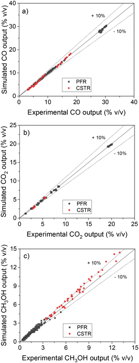Fig. 10 Validation of the ANN₃₀ with steady-state experimental data performed in a PFR¹⁰ and in a CSTR.¹⁸ (a) CO. (b) CO₂. (c) CH₃OH.

The ANN₃₀ coupled with reactor models correctly predicted the experimental data (see Fig. 10), with all points close to the bisection and most points predicted with less than 10% error. Low deviations are seen for the different reactor geometries (PFR and CSTR) and for the varied amounts of methanol produced. A systematic slight overestimation (5–15%) of the methanol points at high production can be observed, with an identical behavior occurring for the MKM (see Fig. S2†).

After confirming that the ANN₃₀ accurately reproduces both the MKM simulations and the experimental data, the computational costs were addressed. In Fig. 11, the average computational time of the MKM and all developed ANNs for one evaluation of the reaction rates is presented. Since the computational time to solve the MKM varies depending on the Jacobian matrix calculation method, it was provided for both the analytical Jacobian (AJ) and numerical Jacobian (NJ) evaluation. Additionally, the computational costs of the formal kinetic model (FKM) from Graaf et al.³¹ were also included as a reference. The confidence interval for a 0.05 level of significance was approximately ±0.7% of the corresponding average value in all cases.

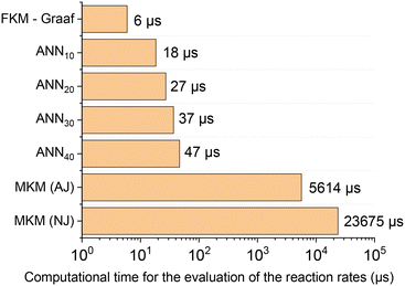Fig. 11 Average computational time of different models to calculate the reaction rates (μs). FKM – Graaf refers to the formal kinetic model developed by Graaf et al.²⁴ The microkinetic model was solved by two approaches: providing the analytical Jacobian matrix (AJ) and calculating the Jacobian matrix numerically (NJ).

The computational costs of the developed ANN₃₀ were two orders of magnitude lower in comparison with the MKM (three, if no analytical Jacobian is provided), a significant improvement. Besides, the computational time of ANN₃₀ is relatively close to the one of a well-known formal kinetic model in the literature³¹ (which is a simplified kinetic approach with lumped parameters). Therefore, the developed ANN is adequate for the combination with complex reactor models, e.g. computational fluid dynamics. In addition, the computational time of the ANN scales linearly with the hidden layer size, being no bottleneck in case larger ANNs are required to learn more complex reaction mechanisms.

4. Summary and conclusions

In this work, a comprehensive methodology to reduce the computational costs of a microkinetic model (MKM) by developing a surrogate artificial neural network (ANN) was presented and successfully demonstrated in a case study of methanol synthesis on Cu/Zn-based catalysts. The ANN accurately reproduced the MKM results and correctly learned the influence of each process parameter in the reaction rates. Thermodynamic consistency was ensured in the model, and the correct description of the equilibrium was demonstrated. As a concluding validation test, real experimental data were accurately described by the model, with most steady-state points reproduced with a relative error lower than 10%.

The computational costs were reduced by 2–3 orders of magnitude when using the ANNs, and they were relatively close to formal kinetic models describing the same system. An additional relevant contribution of this work was the design of a new activation function, which provides non-linearity to the model at significantly lower costs compared to common functions used in ANN development. In addition, neither the proposed function nor its first derivative contain any discontinuity, therefore smoothing out calculations, which is especially beneficial when solving optimization problems.

The proposed methodology should be applicable to reduce the computational costs of other microkinetic models. The resulting ANN enables coupling with catalyst deactivation models and complex reactor models.

Nomenclature

E A,k	Activation energy of reaction k (kJ mol^−1)
f j	Fugacity of component j (bar)
h	Planck constant (kJ s)
I j	Input j of the artificial neural network
K ^0P,n	Equilibrium constant of global reaction n
k b	Boltzmann constant (kJ K^−1)
k ij	Binary interaction parameters (—)
L	Catalyst mass length (m)
MEn	Mean error associated with global reaction n
MSEn	Mean squared error associated with global reaction n
m Cat	Total catalyst mass (kg)
N G	Number of gas phase components (—)
N GR	Number of global reactions (—)
N I	Number of inputs (—)
N R	Number of elementary reactions (—)
N S	Number of surface intermediates (—)
N TP	Number of data points for training the ANN (—)
N P	Total number of data points (—)
n M,Cat	Amount of active sites per catalyst mass (mol kgcat^−1)
ṅ	Total mole flow (mol s^−1)
p 0	Reference pressure (1 bar)
p̂ nw	Parameter of the output layer of output n and cell w
p wj	Parameter of the hidden layer of cell w and input j
R	Universal gas constant (kJ mol^−1 K^−1)
R ^2 n	R ^2 associated with global reaction n
r k	Rate of reaction k (mol kgcat^−1 s^−1)
s w	Value of cell w from the hidden layer (HL)
ŝ w	Value of cell w from the output layer (OL)
T	Temperature (K)
t	Time (s)
w ni	Selected weight of global reaction n and data point i
X j	Conversion of component j (—)
y j	Mole fraction of gas phase component j (—)
β k	Correction term of reaction k to ensure thermodynamic consistency (—)
ΔS^≠k	Entropy barrier of reaction k (kJ mol^−1 K^−1)
θ i	Surface coverage of intermediate i
	Stoichiometric coefficient of species i in the forward direction of reaction k
	Stoichiometric coefficient of species i in the reverse direction of reaction k
ϕ i	Fraction of the site type of surface species i in relation to the total number of sites for carbon-containing compounds (sites a and b)
ω	Acentric factor (—)

Subscripts

ANN	Simulated with the artificial neural network
eq.	Equilibrium
in	Inlet stream or input value
max	Maximum allowed value
min	Minimum allowed value
MKM	Simulated with the microkinetic model
norm	Normalized value
out	Outlet stream or output value

Superscripts

K	Kinetic term
T	Thermodynamic term
+	Forward reaction
−	Reverse reaction

Conflicts of interest

There are no conflicts to declare.

Acknowledgements

We thank Coordenação de Aperfeiçoamento de Pessoal de Nível Superior (CAPES) (Process Nr.: 88881.174609/2018-01) for providing a PhD scholarship for B. L. O. Campos. We acknowledge the financial support of the Conselho Nacional de Desenvolvimento Científico e Tecnológico (CNPq) (Process Nr.: 312248/2022-9). We acknowledge the financial support of the Helmholtz Research Program “Materials and Technologies for the Energy Transition (MTET), Topic 3: Chemical Energy Carriers”. Finally, we acknowledge the support from the KIT-Publication Fund of the Karlsruhe Institute of Technology.

References

1. J. Park, H. S. Kim, W. B. Lee and M.-J. Park, Catalysts, 2020, 10, 655.
2. M. Behrens, F. Studt, I. Kasatkin, S. Kühl, M. Hävecker, F. Abild-Pedersen, S. Zander, F. Girgsdies, P. Kurr, B.-L. Kniep, M. Tovar, R. W. Fischer, J. K. Nørskov and R. Schlögl, Science, 2012, 336, 893–897.
3. J. Fuller, Q. An, A. Fortunelli and W. A. Goddard, III, Acc. Chem. Res., 2022, 55, 1124–1134.
4. S. Wild, B. Lacerda de Oliveira Campos, T. A. Zevaco, D. Guse, M. Kind, S. Pitter, K. Herrera Delgado and J. Sauer, React. Chem. Eng., 2022, 7, 943–956.
5. M. Votsmeier, A. Scheuer, A. Drochner, H. Vogel and J. Gieshoff, Catal. Today, 2010, 151, 271–277.
6. A. Scheuer, W. Hauptmann, A. Drochner, J. Gieshoff, H. Vogel and M. Votsmeier, Appl. Catal., B, 2012, 111–112, 445–455.
7. B. Partopour and A. G. Dixon, Comput. Chem. Eng., 2016, 88, 126–134.
8. E. A. Daymo, M. Hettel, O. Deutschmann and G. D. Wehinger, Chem. Eng. Sci., 2022, 250, 117408.
9. J. M. Blasi and R. J. Kee, Comput. Chem. Eng., 2016, 84, 36–42.
10. M. Bracconi and M. Maestri, Chem. Eng. J., 2020, 400, 125469.
11. B. Partopour, R. C. Paffenroth and A. G. Dixon, Comput. Chem. Eng., 2018, 115, 286–294.
12. F. A. Döppel and M. Votsmeier, Chem. Eng. Sci., 2022, 262, 117964.
13. B. Lacerda de Oliveira Campos, K. Herrera Delgado, S. Wild, F. Studt, S. Pitter and J. Sauer, React. Chem. Eng., 2021, 6, 868–887.
14. F. Studt, M. Behrens and F. Abild-Pedersen, Catal. Lett., 2014, 144, 1973–1977.
15. F. Studt, M. Behrens, E. L. Kunkes, N. Thomas, S. Zander, A. Tarasov, J. Schumann, E. Frei, J. B. Varley, F. Abild-Pedersen, J. K. Nørskov and R. Schlögl, ChemCatChem, 2015, 7, 1105–1111.
16. M. G. Evans and M. Polanyi, Trans. Faraday Soc., 1935, 31, 875–894.
17. H. Eyring, J. Chem. Phys., 1935, 3, 107–115.
18. K. Herrera Delgado, L. Maier, S. Tischer, A. Zellner, H. Stotz and O. Deutschmann, Catalysis, 2015, 5, 871–904.
19. D.-Y. Peng and D. B. Robinson, Ind. Eng. Chem. Fundam., 1976, 15, 59–64.
20. L. Meng and Y.-Y. Duan, Fluid Phase Equilib., 2005, 238, 229–238.
21. L. Meng, Y.-Y. Duan and X.-D. Wang, Fluid Phase Equilib., 2007, 260, 354–358.
22. U. K. Deiters, Fluid Phase Equilib., 2013, 352, 93–96.
23. L. P. de Oliveira, D. Hudebine, D. Guillaume and J. J. Verstraete, Oil Gas Sci. Technol., 2016, 71, 45.
24. C. Seidel, A. Jörke, B. Vollbrecht, A. Seidel-Morgenstern and A. Kienle, Chem. Eng. Sci., 2018, 175, 130–138.
25. Y. Slotboom, M. J. Bos, J. Pieper, V. Vrieswijk, B. Likozar, S. R. A. Kersten and D. W. F. Brilman, Chem. Eng. J., 2020, 389, 124181.
26. N. Park, M.-J. Park, Y.-J. Lee, K.-S. Ha and K.-W. Jun, Fuel Process. Technol., 2014, 125, 139–147.
27. B. Lacerda de Oliveira Campos, K. Herrera Delgado, S. Pitter and J. Sauer, Ind. Eng. Chem. Res., 2021, 60, 15074–15086.
28. I. Chorkendorff and J. W. Niemantsverdriet, Concepts of Modern Catalysis and Kinetics, Wiley, 3rd edn, 2017.
29. E. Goos, A. Burcat and B. Ruscic, New NASA thermodynamic polynomials database, Available at: http://garfield.chem.elte.hu/Burcat/THERM.DAT, (Access in Mar. 2022).
30. A. Chakkingal, P. Janssens, J. Poissonnier, A. J. Barrios, M. Virginie, A. Y. Khodakov and J. W. Thybaut, React. Chem. Eng., 2022, 7, 101–110.
31. G. H. Graaf, E. J. Stamhuis and A. A. C. M. Beenackers, Chem. Eng. Sci., 1988, 43, 3185–3195.

---

Footnote

† Electronic supplementary information (ESI) available. See DOI: https://doi.org/10.1039/d3re00409k

---