Rapid quantitative analysis of petroleum coke properties by laser-induced breakdown spectroscopy combined with random forest based on a variable selection strategy

Abstract

Driven by the “double carbon” strategy, petroleum coke short-term demand is growing rapidly as a negative electrode material for artificial graphite. The analysis of petroleum coke physicochemical properties has always been an important part of its research, encompassing significant indicators such as ash content, volatile matter and calorific value. A strategy based on laser-induced breakdown spectroscopy (LIBS) in combination with chemometrics is proposed to realize the rapid and accurate quantification of the above properties. LIBS spectra of 46 petroleum coke samples were collected, and an original random forest (RF) calibration model was constructed by optimizing the pretreatment parameters. The RF calibration model was further optimized based on variable importance measures (VIM) and variable importance in projection (VIP) methods. After variable selection, the elemental spectral lines related to ash content, volatile matter and calorific value modeling were screened out, thus initially exploring the correlation between these properties and elements. Under the optimized spectral pretreatment method, VI threshold and model parameters, the mean relative error (MRE_P) of the prediction set of ash content, volatile matter and calorific value were 0.0881, 0.0527 and 0.006, the root mean square error (RMSE_P) of the prediction set of ash content, volatile matter and calorific value were 0.0471%, 0.6178% and 0.2697 MJ kg⁻¹, respectively, and the determination coefficient (R_P²) of the prediction set was 0.9187, 0.9820 and 0.9510, respectively. The combination of LIBS technology and chemometric methods can provide powerful technical means for the analysis and evaluation of the physicochemical properties of petroleum coke.

---

1. Introduction

Petroleum coke is a granular, columnar or needle-like carbon substance composed of tiny graphite crystals, including green coke, calcined coke and needle-like coke.^1–3 It is used as a raw material for various industries, including prebaked anodes, industrial silicon, negative materials for new energy lithium batteries and so on.^4–6 The analysis of petroleum coke physicochemical properties has always been crucial in its research, including ash content, volatile matter and calorific value. Ash content significantly impacts electrolytic energy consumption, loss and aluminum purity of anode products. Volatile matter is a measure of coking degree and plant economy. Meanwhile, calorific value reflects the combustion characteristics of petroleum coke. Therefore, the research on ash content, volatile matter, and calorific value holds significant importance in guiding the rational, clean, and efficient utilization of petroleum coke.^7,8 Analysis of the petroleum coke properties can be conducted through direct property determination or elemental content analysis. Direct property determination method covers traditional high-temperature calcination and oxygen bomb calorimetry method, and rapid techniques such as X-ray, γ-ray and microwave methods.^9–12 Commonly used methods for elemental content detection include wavelength dispersive X-ray fluorescence spectroscopy (WD-XRF), atomic absorption spectroscopy (AAS), inductively coupled plasma techniques (ICP-MS, ICP-OES), etc.^13–16 Although the above methods have remarkable detection sensitivity and accuracy, almost all of them target a single analytical index and involve complicated, time-consuming, and laborious sample preparation. Therefore, a rapid, simple pretreatment process and multi-element simultaneous detection method for petroleum coke analysis is required.

Laser-induced breakdown spectroscopy (LIBS) as a mature atomic spectral analysis technique,^17,18 has the obvious advantage of without complicated sample pretreatment and multi-element simultaneous analysis. Moreover, it has the advantages of real-time, fast, in situ and micro-damage, and has significant application value in key scientific fields such as deep space exploration, archaeological science, metallurgical analysis, environmental monitoring, geological exploration and biomedicine.^19–24 Petroleum molecular analysis is an important application field of LIBS. Currently, LIBS technology is mainly utilized for elemental analysis in the research of petroleum coke.^25,26 In 2021, Zhang et al. innovatively applied LIBS technology to the detection of V, Fe, and Ni in petroleum coke.²⁵ Subsequently, Lu et al. optimized the content of stearic acid binder in petroleum coke tablets and found that the performance of LIBS was significantly improved when stearic acid accounted for 30 wt%.²⁶ However, there is no report on the prediction of ash content, volatile matter, and calorific value of petroleum coke using LIBS.

Recently, the combination of spectroscopy and chemometrics has shown high feasibility in the analysis of petroleum molecules, aiming at material elements, properties and structures.^27,28 Aiming at the chemical composition diversity and spectral complexity of petroleum coke samples, an random forest (RF) calibration model based on ensemble learning and decision tree is used to achieve the requirements of rapid quantitative analysis of physicochemical properties of petroleum coke. Chen et al. compared RF, partial least squares (PLS), and least squares support vector machine (LSSVM) for predicting Zn, Cu, and Ni properties in a single micro-scale suspended particle.²⁹ The results indicated that RF exhibited superior performance, with the mean relative error (MRE) values of 0.0862, 0.1020, and 0.1323, respectively. Furthermore, Wang et al. compared the performance of multiple linear regression (MLR), RF, and deep fully connected neural network (DNN) in predicting coal structures.³⁰ In tests conducted with 300 and 1200 sample groups, RF demonstrated the highest accuracy of 83% and 86%, respectively, highlighting its advantages in precision and noise resistance.

Based on the actual demand for rapid and accurate analysis of petroleum coke properties, an optimized RF calibration model was proposed, integrating combined pretreatment strategy with variable importance measures (VIM) and variable importance in projection (VIP) for rapid determination of ash content, volatile matter, and calorific value. This study collected various petroleum coke types, such as sponge coke, shot coke, needle coke, calcined coke and pitch coke. Firstly, the LIBS spectrum was acquired from 46 samples, and an initial RF calibration model was constructed by optimizing pretreatment parameters. Secondly, by selecting appropriate thresholds for VIM and VIP, the model can be further optimized, eliminating irrelevant variables and retaining important variables related to analyte composition. Model performance was evaluated using determination coefficient (R²), MRE, and the root mean square error (RMSE). Finally, model stability was verified by calculating the values of the ratio of the standard deviation of the response variable to the RMSE_P (RPD), the ratio of the RMSE_P to the range (RER), and the relative standard deviation (RSD), which provides a novel approach for the petroleum coke properties analysis.

2. Materials and methods

2.1 Sample collection and preparation

The present article involved 46 samples of petroleum coke, in which 29 samples (no. 1–29) were mixed in different proportions from five kinds of petroleum coke standard sample powders (ZBM131, ZBM132, ZBM133, ZBM134 and ZBM135 petroleum coke standard samples purchased from Jinan Zhongbiao Technology Co., Ltd). And 17 actual samples (no. 30–46) provided by Shandong Zhigu Carbon Research Institute Co., Ltd.

For standard samples, a certain amount of powder was weighed according to different proportions and ball-milled and mixed evenly by QM-3SP2 planetary ball mill (Nanjing Laibu Technology Industrial Co., Ltd). For actual samples, a certain amount of solid block samples was weighed and grinded with planetary ball mill. The mixed mode is bidirectional interval alternation, the mixed time is set to 60 minutes, and the rotating speed is set to 450 rpm so that it is finely ground and sieved with a 200 mesh sieve. 20 g sieved powder samples were taken out to prepare the reference values determination of ash content, volatile matter and calorific value. Before LIBS spectral acquisition, each sieved petroleum coke powder sample was pressed into tablets by PC-24 tablet press (Pinchuang Technology Co., Ltd, the maximum pressure is 30 MPa) under 20 MPa for 5 min.

2.2 Reference value determination

For the determination of the reference value of ash content, petroleum coke samples were weighed and then were put into a muffle furnace, heated to 815 °C at a certain speed, ashed and burned until the quality is constant, and the mass fraction of the residue in the original quality of petroleum coke is taken as the reference value of ash content. For the determination of the reference value of volatile matter, sample powder was placed in a porcelain crucible with a cover, and heated for 7 minutes at 900 °C without air, so that the decreasing mass minus the mass fraction of water content in the coke mass is taken as the volatile matter of petroleum coke. The calorific value mentioned in this article is oxygen bomb calorific value. In order to reduce the error caused by a single test, each sample was tested three times. In the calculation process, the average result of three tests is taken as the analysis result. Table 1 presents the reference values of ash content, volatile matter and calorific value of each petroleum coke sample. During the modeling process, the training set and the prediction set were divide from 46 samples at a ratio of 3 : 1 by Kennard–Stone (KS) algorithm, and the prediction set was marked as superscript a.

Table 1 Reference values of ash content, volatile matter and calorific value in petroleum coke

No.	Ash (wt%)	Volatile matter (wt%)	Calorific value (MJ kg^−1)	No.	Ash (wt%)	Volatile matter (wt%)	Calorific value (MJ kg^−1)
a Selected for prediction sample.
1	0.35	18.88	36.26	24^a	0.49	15.57	35.72
2	0.34	10.48	35.01	25	0.54	16.62	35.86
3	0.30	14.08	35.65	26^a	0.42	17.37	36.06
4	0.26	4.02	33.75	27	0.47	10.85	35.06
5^a	0.28	11.85	34.96	28^a	0.42	11.94	35.23
6	0.28	15.03	35.63	29^a	0.50	12.58	35.26
7	0.30	6.34	34.28	30^a	0.50	11.00	35.57
8	0.40	8.32	34.59	31^a	0.25	9.23	35.51
9^a	0.25	5.67	34.08	32	0.24	10.15	34.90
10^a	0.34	8.94	34.54	33	1.33	13.22	35.53
11	0.28	11.52	35.12	34	0.87	10.59	34.92
12	0.35	7.86	33.81	35	0.40	15.99	35.64
13	0.24	11.74	34.63	36	0.20	12.16	35.77
14	0.33	15.39	35.44	37^a	0.88	1.65	31.89
15	0.36	4.17	33.40	38	1.12	1.46	32.46
16^a	0.38	6.55	33.83	39	0.66	1.29	32.54
17	0.36	8.46	34.37	40	1.10	1.15	32.55
18	0.38	5.73	33.52	41	0.72	1.39	32.64
19	0.46	8.69	34.22	42	1.87	1.33	32.41
20	0.50	11.59	34.89	43	0.68	1.19	32.17
21	0.36	14.00	35.54	44	0.58	9.24	34.99
22^a	0.36	16.15	35.83	45	0.45	54.74	37.31
23	0.39	17.62	36.02	46	0.59	42.12	38.09

---

2.3 LIBS spectrum collection

In this study, a commercially integrated LIBS instrument was employed. A Nd:YAG laser (LPS-1064-S) with a pulse width of 6 ns was used as the excitation light source, with a pulse energy of 150 mJ, laser spot diameter of 0.2 mm and a pulse repetition rate of 1 Hz. During the determination, the sample was placed directly on an automatically adjustable 3D displacement platform. The laser beam focused on the sample surface through the cage optical path, ablated the surface to generate plasma. Subsequently, the plasma radiation light is coupled to the optical fiber through the cage optical path, and then transmitted to the spectrometer (Avantes, AvaSpec-ULS4096CL-7-JLU, spectral ranges: 200–923 nm, minimum gate width: 9 μs, resolution: 0.07–0.18 nm) for analysis. To ensure the stability and accuracy of spectral measurements, following the configuration recommended in relevant literature,^31–33 each spectrum was acquired by averaging 10 laser pulses. The integration time was fixed to 150 μs. The optimal delay time was chosen based on the average signal-to-noise ratio (SNR) of each element across various delay time. The optimization results presented in Fig. S1,† revealing a final delay time of 1.5 μs. As the accuracy and precision of LIBS spectrum are easily affected by sample inhomogeneity, 50 different positions of each tablets are randomly selected for determination. The analytical spectra were obtained by averaging 10 spectra, and 230 spectral data were obtained from 46 samples.

2.4 Random forest

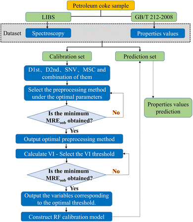
In this work, RF was used to establish calibration models for the ash content, volatile matter, and calorific value of petroleum coke. RF, proposed by Leo Breiman in 2001, is an algorithm based on Bagging integrated learning theory, developed from decision trees. It is commonly used to deal with classification and regression problems and has strong generalization energy.^34,35 There are two important parameters in the modeling process of RF, namely decision tree nodes number (m_try) and decision tree numbers (n_tree). In the training stage, 34 sample sets were randomly selected from 46 samples by the bootstrap resampling strategy as calibration set for the construction of 34 regression trees. In this step, the remaining sample sets were used as prediction set to calibrate the performance of each tree. The final prediction result of the RF model was the average result of all individual tree predictions. Fig. 1 shows a schematic diagram of quantitative analysis of petroleum coke properties by RF combined with pretreatment and variable selection methods. In this article, MRE_oob, RMSE_oob and R_oob² represents MRE, RMSE and R² calculated for out-of-bag (oob) samples of the model, respectively.

Fig. 1 The diagram of LIBS combined with random forest for properties analysis of petroleum coke.

3. Results and discussion

3.1 LIBS spectral analysis of petroleum coke samples

Fig. 2 presents the average normalized spectrum of the denoised petroleum coke sample 3#, and the characteristic spectral lines of elements in petroleum coke sample were identified based on the NIST database.³⁶ From Fig. 2, the trace elements in petroleum coke samples are mainly Fe, Al, Ca, Na, S, Ti, etc. Most of these elements are inherent in crude oil, while some of them enter during the coking process of petroleum coke and the storage and transportation of raw materials. Some of the elements exhibit lower spectral intensities, such as Fe I (358.119 nm), Ca I (422.673 nm) and Ti I (422.94 nm). Furthermore, there are many interference peaks around Fe, Ca, Ti, and other elements, which will lead to inaccurate quantitative and classification results. This indicates the need for preprocessing the spectrum.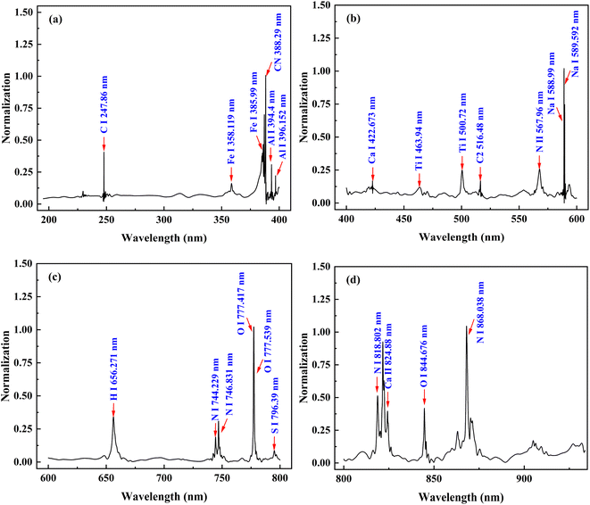

Fig. 2 Averaged LIBS spectrum of 3# petroleum coke sample based on noise reduction treatment ((a) 200–400 nm; (b) 400–600 nm; (c) 600–800 nm; (d) 800–935 nm).

3.2 The selection and optimization of preprocessing methods

During the LIBS spectral acquisition process, various factors such as instrument operating conditions and environmental influences can lead to phenomena such as baseline drift, noise, and overlapping peaks in the spectra. These issues will affect the accuracy of the quantitative analysis results. Consequently, it is crucial to preprocess the LIBS spectra before constructing calibration models, in order to ensure more accurate predictive performance of the models. Given the complexity of the petroleum coke sample substrate, there may be matrix effects caused by the different particle sizes of the samples. Standard normal variate transformation (SNV) and multivariate scattering correction (MSC) can effectively eliminate spectral differences caused by different solid particle sizes and surface scattering levels. Taking the spectral matrix derivative is an effective means to eliminate baseline drift and distinguish overlapping peaks. These methods effectively correct matrix effect and background interference, and eliminate scattering effects. Therefore, preprocessing methods such as the first derivative (D1st), second derivative (D2nd), SNV, and MSC are selected to analyze the original spectra. Merely using default parameter values for these preprocessing methods does not yield optimal preprocessing results, thus necessitating parameter optimization. MRE_oob, RMSE_oob and R_oob² are used as evaluation indices, with MRE_oob serving as the main evaluation index, whereas RMSE_oob and R_oob² serving as the auxiliary evaluation indices.

Taking the derivative of spectral matrix is an effective means to eliminate baseline drift, and distinguish overlapping peaks. The parameter optimization process of D1st is depicted in Fig. 3. As shown in Fig. 3(a), with the increase in smoothing points, the MRE_oob and RMSE_oob of the RF calibration model for ash content exhibit a trend of initial decrease, followed by an increase, and then a subsequent decrease. When the smoothness point is 13, the RF calibration model shows better predictions (R_oob² = 0.8233, MRE_oob = 0.1558, RMSE_oob = 0.1585). For volatile matter analysis, the optimal smoothing point is 25 and the RF calibration model obtained better prediction results (R_oob² = 0.9695, MRE_oob = 0.1708, RMSE_oob = 2.2174). For calorific value analysis, the optimal smoothing point is 25, and the RF calibration model obtains better prediction results (R_oob² = 0.9837, MRE_oob = 0.0036, RMSE_oob = 0.1836).

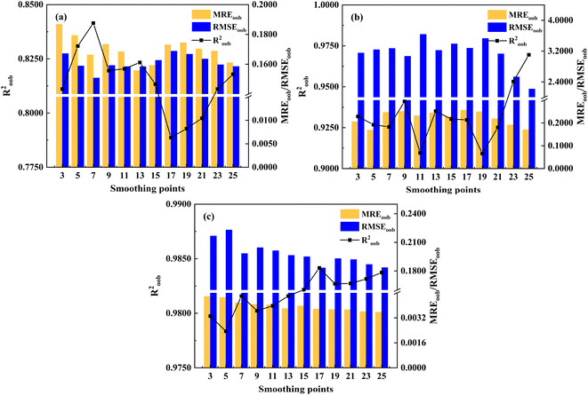Fig. 3 Prediction results of RF calibration model based on different D1st smoothing points ((a) ash content; (b) volatile matter; (c) calorific value).

Simultaneously, the impact of D2nd smoothing points on the analysis results of RF calibration models was discussed. Fig. 4 shows the impact of different smoothing points based on D2nd on the accuracy of the calibration model analysis results for ash content, volatile matter, and calorific value. As can be seen from Fig. 4, with the smoothing point increasing, the MRE_oob of the RF calibration model of ash content, volatile matter, and calorific value shows a trend of initial increase followed by a decrease. For ash content analysis, the RF calibration model showed better predictions (R_oob² = 0.8518, MRE_oob = 0.1550, RMSE_oob = 0.1455) when the smoothing point was 15. For volatile matter analysis, the optimal smoothing number was 9, and the model obtained better predictions (R_oob² = 0.9521, MRE_oob = 0.2109, RMSE_oob = 2.5631). For calorific value analysis, the optimal smoothing number was 19, and the RF calibration model obtained better prediction results (R_oob² = 0.9838, MRE_oob = 0.0037, RMSE_oob = 0.1866). In summary, by optimizing the selection of smoothing points for D1st and D2nd, the prediction accuracy of the RF calibration models for ash content, volatile matter, and calorific value analysis can be significantly improved.

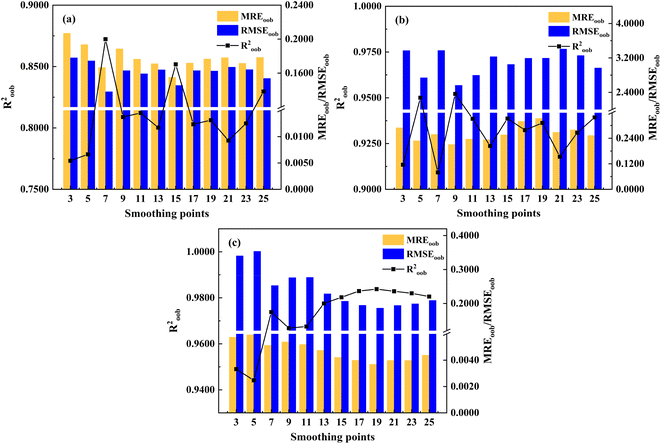Fig. 4 Prediction results of RF calibration model based on D2nd different smoothing points ((a) ash content; (b) volatile matter; (c) calorific value).

Due to the diversity of spectral interference causes and effects, a single pretreatment method may be insufficient to suppress the effects of spectral interferences on modeling effectiveness.³⁷ Thus, the impact of spectral preprocessing combination strategies on the predictive performance of the RF calibration models was further explored (as shown in Fig. 5). Fig. 5 shows that for the ash content model, SNV corresponds to the minimum MRE_oob and RMSE_oob, and D2nd to the maximum R_oob². Consequently, the combination of D2nd and SNV preprocessing methods was selected to train the ash content RF model. For volatile matter model, D1st combined with MSC pretreatment method corresponds to the minimum RMSE_oob and MRE_oob, and the maximum R_oob². However, the prediction result of D1st combined with MSC is inferior to that of MSC alone, which may be due to the over-fitting of the training data caused by the optimization of model parameters, thus reducing the generalization effect of the model. For calorific value model, D1st combined with MSC pretreatment method corresponds to the minimum RMSE_oob and MRE_oob, and the maximum R_oob². Therefore, the RF model of calorific value is trained by selecting D1st combined with MSC pretreatment method.

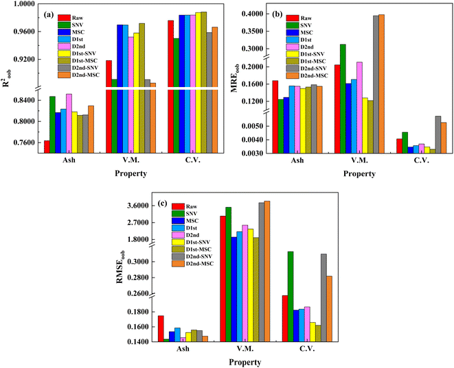Fig. 5 Effects of different preprocessing methods on the predictive performance of RF calibration model (note: Ash: ash content, V.M.: volatile matter, C.V.: calorific value).

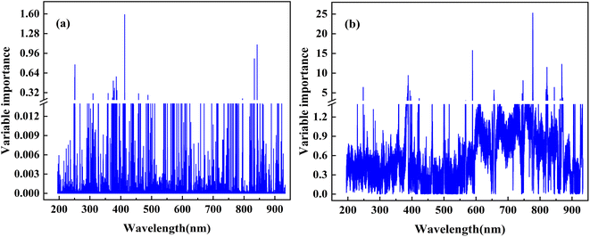
3.3 Selection and optimization of input variables

In the modeling process, some irrelevant variables do not contribute to the model establishment and even lead to increased modeling time, thereby affecting the stability and predictive accuracy of the calibration model. Therefore, extracting and optimizing input variables is critical for improving the predictive performance of the model. For VIM and VIP variable selection methods, the VI value of each input variable is typically calculated when creating RF calibration models. Fig. 6 illustrates the relationship between the VI value and the LIBS wavelengths.

Fig. 6 The RF model VI value selected of the ash content ((a) VIM; (b) VIP).

Based on the optimal spectral preprocessing combination strategy, a comparison was conducted to assess the influence of the VI thresholds in the VIM/VIP algorithms on the predictive results of the RF calibration model. Fig. 7 examines the performance of different VI thresholds on the VIM/VIP-RF models for predicting three properties of petroleum coke. For ash content and volatile matter analysis, the VIM-RF model achieved better predictive performance. From Fig. 7(a), as the VI values increase, the MRE_oob values initially decrease and then increase. A minimum MRE_P is achieved at a threshold of 0.006 (R_P² = 0.9187; MRE_P = 0.0881; RMSE_P = 0.0471). Therefore, a VI threshold of 0.006 is selected as the input variable for constructing the VIM-RF (ash content) calibration model. In contrast, for volatile matter analysis, the MRE_oob value initially increases and then decreases with increasing VI threshold. When the threshold is 0.08, MRE_P is at its minimum (R_P² = 0.9820; MRE_P = 0.0527; RMSE_P = 0.6178). Therefore, the VI threshold value of 0.08 is selected as the input variable, and the VIM-RF (V.M.) calibration model is constructed. For calorific value analysis, VIP-RF model achieves better prediction performance. Fig. 7(b) shows that as the VI threshold increases, the MRE_oob value first increases and then decreases. As the threshold is 1.0, MRE_oob is the minimum (R_P² = 0.9510; MRE_P = 0.0060; RMSE_P = 0.2697). Thus, the VI threshold of 1.0 is selected as the input variable and the VIP-RF (C.V.) calibration model is constructed.

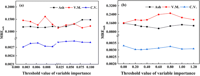Fig. 7 Predictive performance of the RF model of ash content, volatile matter, and calorific values under different thresholds ((a) VIM; (b) VIP).

After comparing the feature-selected spectral lines with the original spectra, the elemental spectral lines related to ash content modeling are selected, such as Fe I 358.12 nm, 385.99 nm, AI I 394.40 nm, 396.15 nm, Ca I 824.88 nm, S I 796.39 nm. Notably, the Fe elemental spectral lines have a large VI value. Interestingly, although a significant VI value was observed near the peak of the Si element at approximately 250 nm, no Si elemental peak was evident in Fig. 2. It is speculated that the Si element peak may be obscured in the Fig. 2 due to excessive noise reduction. For volatile matter, the spectral lines of C, H, O and N have the greatest correlation with modeling after variable selection, and the VI value is about 40. The spectral lines Fe, Ca and Ti of metal elements also show correlation, but the VI value is lower, indicating that non-metallic elements may play a more dominant role in the modeling of volatile matter. For calorific value, the spectral lines of elements with large VI value are mainly C, O, N, and CN, which proves that there is a strong correlation between these elements and calorific value, and metal elements such as Fe, Ca and Na also have certain correlation.

3.4 Verification of prediction performance of different models

After spectral preprocessing and variable selection, the RF calibration models for ash content (D2nd-SNV-VIM-RF), volatile matter (MSC-VIM-RF), and calorific value (D1st-MSC-VIP-RF) exhibited superior predictive performance, as shown in Table 2. The R_oob² for ash content improved from 0.7635 to 0.8924, an increase of 16.9%, while MRE_oob decreased from 0.1679 to 0.1167, a reduction of 30.5%. Similarly, RMSE_oob decreased from 0.1748 to 0.1186, a decrease of 32.2%. For volatile matter, R_oob² increased from 0.9183 to 0.9781, an enhancement of 6.5%, while MRE_oob decreased from 0.2046 to 0.1153, a substantial reduction of 43.6%. RMSE_oob also decreased significantly, from 3.0454 to 1.6333, a drop of 46.4%. Regarding calorific value, R_oob² increased from 0.9759 to 0.9838, an increment of 0.8%. Meanwhile, MRE_oob decreased from 0.0041 to 0.0031, a decrease of 24.4%, and RMSE_oob also decreased from 0.2164 to 0.1796, a reduction of 17.0%. These results demonstrate that appropriate preprocessing methods combined with variable selection strategies can effectively enhance the predictive performance of the models.

Table 2 Predictive performance of RF model after optimal spectral preprocessing and variable selection

Property	Model	Roob^2	MREoob	RMSEoob	RP^2	MREP	RMSEP	RPD	RSD (%)	RER
Ash	D2nd-SNV-VIM-RF	0.8924	0.1167	0.1186	0.9187	0.0881	0.0471	3.82	2.90	14.62
V.M.	MSC-VIM-RF	0.9781	0.1153	1.6333	0.9820	0.0527	0.6178	7.21	3.88	25.45
C.V.	D1st-MSC-VIP-RF	0.9838	0.0031	0.1796	0.9510	0.0060	0.2697	4.20	0.22	15.46

---

It can be seen from the table that the idea of VIM/VIP variable selection after preprocessing method is feasible. Fig. 8 shows the relationship between reference values and predicted values under different RF calibration models. R_P² of ash content, volatile matter and calorific value increased by 35.8%, 7.46% and 9.15%, respectively. MRE_P decreased significantly, by 55.2%, 43.5% and 41.7%, respectively. RMSE_P decreased by 50.6%, 60.7% and 35.1%, respectively. For ash content analysis, a D2nd-SNV-VIM-RF calibration model was established, achieving a low prediction RSD of 2.9%. The RPD value of the model, representing the ratio of the standard deviation of the response variable to RMSE_P,³⁸ was 3.82, indicating high accuracy. Generally, a RPD value exceeding 3 indicates acceptable prediction results. Furthermore, the RER value (RER = R_n/RMSE_P,³⁹ where R_n is the concentration range) reached 14.62, far exceeding the threshold of 10, demonstrating the model suitability for quality control applications and high robustness. For volatile matter analysis, an MSC-VIM-RF model exhibited a prediction performance with an RSD of 3.88%. The RPD value was calculated as 7.21, and the RER value was 25.45. For calorific value analysis, a D1st-MSC-VIP-RF model was established, the predicted performance of the calibration model being RSD 0.22%. The RPD value was 4.20, and the RER value was 15.47, both indicating high precision and strong robustness of the model.

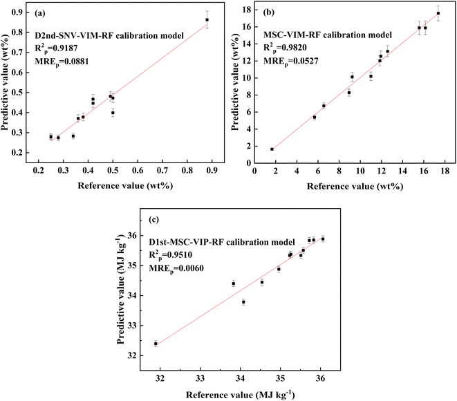Fig. 8 The relationship between the reference value and predictive value obtained by different RF calibration models ((a) ash content; (b) volatile matter; (c) calorific value).

Furthermore, the model prediction results were compared with those of similar complex systems. Firstly, in the LIBS-based analysis of petroleum coke, compared to the previous research by Lu et al., the currently established models for ash content, volatile matter, and calorific value exhibited lower RSD values of 2.90%, 3.88%, and 0.22%, respectively, compared to their models for V, Na, and Ca element analysis, which had RSD values of 3.65%, 4.38%, and 5.53%.²⁶ This demonstrates the superior stability of the current models. Additionally, the RMSE_P values of the current models were 0.0471% for ash content, 0.6178% for volatile matter, and 0.2697 MJ kg⁻¹ for calorific value. When compared to approximate analysis results based on coal, He et al. reported an RMSE_P of 0.9687% for ash content and 1.3218% for volatile matter using a KELM model based on a primary spectral fusion strategy.⁴⁰ Zhang et al. employed four calibration models, namely partial least squares regression (PLSR), support vector regression (SVR), artificial neural networks (ANN), and principal component regression (PCR), to quantitatively analyze 40 coal samples, achieving RMSE_P values of 0.69% for ash content, 0.87% for volatile matter, and 0.56 MJ kg⁻¹ for calorific value.⁴¹ The results obtained in this research further validating the effectiveness of the established calibration models.

Finally, the validity and limitation of the model in the study of ash content, volatile matter and calorific value were discussed. Considering the solid flake characteristics of petroleum coke samples, SNV and MSC effectively eliminate spectral differences arising from particle size and surface scattering. Additionally, derivative techniques correct for matrix effects and background interference. VIM and VIP feature selection techniques facilitate the identification of key spectral features, simplifying the model structure and enhancing prediction accuracy. Furthermore, the RF algorithm excels in handling high-dimensional data and nonlinear relationships, providing valuable variable importance assessments. Nevertheless, the quality and integrity of data are crucial, and different datasets may necessitate adjustments in preprocessing methods. Moreover, the RF algorithm may encounter challenges such as overfitting and computational efficiency. Therefore, it is crucial to comprehensively consider these factors when applying the model to practical petroleum coke detection.

4. Conclusion

LIBS technique combined with RF calibration model has successfully predicted the ash content, volatile matter and calorific value of petroleum coke. During the research, LIBS spectral data were collected from 46 samples, including standard and actual petroleum coke samples. Then, the impact of spectral preprocessing combination strategies on RF-calibration model predictive results was discussed. Finally, irrelevant variables were maximally removed from the spectral data through variable selection methods VIP and VIM. The results showed that the D2nd-SNV-VIM-RF calibration model obtained the best predictive results for ash content analysis (R_P² = 0.9187; MRE_P = 0.0881; RMSE_P = 0.0471). For volatile matter analysis, the MSC-VIM-RF calibration model obtained the best predictive result (R_P² = 0.9820, MRE_P = 0.0527, RMSE_P = 0.6178). For calorific value analysis, the D1st-MSC-VIP-RF calibration model obtained the best predictive result (R_P² = 0.9510, MRE_P = 0.0060, RMSE_P = 0.2697). Further research shown that pretreatment methods, relevant parameters and combination strategies have great influence on the predictive results of RF calibration model. Generally speaking, the combination of LIBS and chemometric algorithms can improve the research accuracy in quantitatively determining the chemical composition of petroleum coke.

Author contributions

Shunfan Hu: methodology, sample, experiment, data collection, writing-original draft preparation. Jianming Ding: data curation, investigation. Yan Dong: writing-review & editing. Tianlong Zhang: writing-review & editing. Hongsheng Tang: funding acquisition, supervision and writing-review & editing. Hua Li: funding acquisition, supervision, and project administration.

Conflicts of interest

There are no conflicts of interest to declare.

Acknowledgements

This work was supported by the National Natural Science Foundation of China [no. 22173071 and 22073074].

References

1. H. Al-Haj Ibrahim, Recent Adv. Petrochem. Sci., 2017, 3, 555619.
2. Z. You, J. Xiao, Q. Mao, X. Zhang and Q. Zhong, Fuel, 2022, 330, 125521.
3. H. Liu, S. Jiao, W. Liu, B. W. Biney, F. Wang, K. Chen, A. Guo and Z. Wang, J. Anal. Appl. Pyrolysis, 2022, 162, 105454.
4. H. Ran, M. Elchalakani, M. A. Sadakkathulla, J. Cai and T. Xie, Constr. Build. Mater., 2023, 407, 133513.
5. C. Kumar, A. Gupta, P. Saharan, M. Singh and S. R. Dhakate, Diamond Relat. Mater., 2023, 140, 110433.
6. K. Nanaji, A. Nirogi, P. Srinivas, S. Anandan, R. Vijay, R. N. Bathe, M. Pramanik, K. Narayan, B. Ravi and T. N. Rao, J. Energy Storage, 2022, 55, 105650.
7. B. Wang, W. Li, C. Ma, W. Yang, D. Pudasainee, R. Gupta and L. Sun, J. Energy Inst., 2022, 102, 1–13.
8. V. Lazic, M. Romani, L. Pronti, M. Angelucci, M. Cestelli-Guidi, M. Mangano and R. Fantoni, Spectrochim. Acta, Part B, 2023, 201, 106601.
9. C. J. Donahue and E. A. Rais, J. Chem. Educ., 2009, 86, 222–224.
10. F. Brown and S. A. Jones, Adv. X-Ray Anal., 1979, 23, 57–63.
11. M. Yazdi and S. A. Esmaeilnia, Int. J. Coal Geol., 2003, 55, 151–156.
12. N. G. Cutmore, D. A. Abernethy and T. G. Evans, J. Microw. Power Electromagn. Energy, 1989, 24, 79–90.
13. K. Tsuji, in Encyclopedia of Analytical Science, ed. P. Worsfold, C. Poole, A. Townshend and M. Miró, Academic Press, Oxford, 3rd edn, 2019, pp. 459–470,  DOI:10.1016/B978-0-12-409547-2.14477-4.
14. S. L. C. Ferreira, M. A. Bezerra, A. S. Santos, W. N. L. dos Santos, C. G. Novaes, O. M. C. de Oliveira, M. L. Oliveira and R. L. Garcia, TrAC, Trends Anal. Chem., 2018, 100, 1–6.
15. J.-L. Todolí, in Encyclopedia of Analytical Science, ed. P. Worsfold, C. Poole, A. Townshend and M. Miró, Academic Press, Oxford, 3rd edn, 2019, pp. 209–217,  DOI:10.1016/B978-0-12-409547-2.14473-7.
16. M. L. Fernández-Sánchez, in Encyclopedia of Analytical Science, ed. P. Worsfold, C. Poole, A. Townshend and M. Miró, Academic Press, Oxford, 3rd edn, 2019, pp. 169–176,  DOI:10.1016/B978-0-12-409547-2.14542-1.
17. X. Li, L. Zhang, Z. Tian, Y. Bai, S. Wang, J. Han, G. Xia, W. Ma, L. Dong, W. Yin, L. Xiao and S. Jia, J. Anal. At. Spectrom., 2020, 35, 2928–2934.
18. A. W. Miziolek, V. Palleschi and I. Schechter, Laser Induced Breakdown Spectroscopy, Cambridge University Press, Cambridge, 2006.
19. X. Wan, R. Yuan, H. Wang, Y. Cheng, J. Jia, R. Shu, W. Xu, C. Li, Y. Xin, H. Ma, P. Fang and Z. Ling, Anal. Chem., 2021, 93, 7970–7977.
20. F. Ruan, T. Zhang and H. Li, Appl. Spectrosc. Rev., 2019, 54, 1–29.
21. T. Zhang, S. Wu, J. Dong, J. Wei, K. Wang, H. Tang, X. Yang and H. Li, J. Anal. At. Spectrom., 2015, 30, 368–374.
22. Y. Zhang, T. Zhang and H. Li, Spectrochim. Acta, Part B, 2021, 181, 106218.
23. T. Chen, T. Zhang and H. Li, TrAC, Trends Anal. Chem., 2020, 133, 116113.
24. B. Busser, S. Moncayo, J.-L. Coll, L. Sancey and V. Motto-Ros, Coord. Chem. Rev., 2018, 358, 70–79.
25. W. Zhang, Z. Zhuo, P. Lu, T. Sun, W. Sun and J. Lu, Spectrochim. Acta, Part B, 2021, 177, 106076.
26. P. Lu, Z. Zhuo, W. Zhang, T. Sun, W. Sun and J. Lu, Spectrochim. Acta, Part B, 2022, 190, 106388.
27. K. T. Butler, D. W. Davies, H. Cartwright, O. Isayev and A. Walsh, Nature, 2018, 559, 547–555.
28. L. Verma, F. Kremer and K. Chevalier-Jabet, Prog. Nucl. Energy, 2023, 160, 104686.
29. T. Chen, T. Zhang, C. Niu, T. Feng, H. Tang, X. Cheng and H. Li, Anal. Chem., 2022, 94, 17595–17605.
30. Z. Wang, Y. Cai, D. Liu, F. Qiu, F. Sun and Y. Zhou, Int. J. Coal Geol., 2023, 268, 104208.
31. C. Yan, T. Zhang, Y. Sun, H. Tang and H. Li, Spectrochim. Acta, Part B, 2019, 154, 75–81.
32. J. Qi, T. Zhang, H. Tang and H. Li, Spectrochim. Acta, Part B, 2018, 149, 288–293.
33. C. Yan, J. Liang, M. Zhao, X. Zhang, T. Zhang and H. Li, Anal. Chim. Acta, 2019, 1080, 35–42.
34. L. Breiman, Mach. Learn., 2001, 45, 5–32.
35. Z. Sun, G. Wang, P. Li, H. Wang, M. Zhang and X. Liang, Expert Syst. Appl., 2024, 237, 121549.
36. https://physics.nist.gov/PhysRefData/Handbook/periodictable.htm.
37. M. Guo, M. Li, H. Fu, Y. Zhang, T. Chen, H. Tang, T. Zhang and H. Li, Spectrochim. Acta, Part A, 2023, 287, 122057.
38. B. M. Nicolaï, K. Beullens, E. Bobelyn, A. Peirs, W. Saeys, K. I. Theron and J. Lammertyn, Postharvest Biol. Technol., 2007, 46, 99–118.
39. P. Williams and D. Sobering, Near Infrared Spectroscopy: The Future Waves, 1996, pp. 185–188.
40. T. He, J. Liang, H. Tang, T. Zhang, C. Yan and H. Li, Spectrochim. Acta, Part B, 2021, 178, 106112.
41. Y. Zhang, Z. Xiong, Y. Ma, C. Zhu, R. Zhou, X. Li, Q. Li and Q. Zeng, Anal. Methods, 2020, 12, 3530–3536.

---

Footnote

† Electronic supplementary information (ESI) available. See DOI: https://doi.org/10.1039/d4ra02873b

---