DOI:
10.1039/D4RA02475C
(Paper)
RSC Adv., 2024,
14, 19331-19348
Predicting micropollutant removal through nanopore-sized membranes using several machine-learning approaches based on feature engineering
Received
1st April 2024
, Accepted 5th June 2024
First published on 17th June 2024
Abstract
Predicting the efficacy of micropollutant separation through functionalized membranes is an arduous endeavor. The challenge stems from the complex interactions between the physicochemical properties of the micropollutants and the basic principles underlying membrane filtration. This study aimed to compare the effectiveness of a modest dataset on various machine learning tools (ML) tools in predicting micropollutant removal efficiency for functionalized reverse osmosis (RO) and nanofiltration (NF) membranes. The inherent attributes of both the micropollutants and the membranes are utilized as input factors. The chosen ML tools are supervised algorithm (adaptive network-based fuzzy inference system (NF), linear regression framework (linear regression (LR)), stepwise linear regression (SLR) and multivariate linear regression (MVR)), and unsupervised algorithm (support vector machine (SVM) and ensemble boosted tree (BT)). The feature engineering and parametric dependency analysis revealed that characteristics of micropollutants, such as maximum projection diameter (MaxP), minimal projection diameter (MinP), molecular weight (MW), and compound size (CS), exhibited a notably positive impact on the correlation with removal efficiency. Model combination with key variables demonstrated high prediction accuracy in both supervised and unsupervised ML for micropollutant removal efficiency. An NF-grid partitioning (NF-GP) model achieved the highest accuracy with an R2 value of 0.965, accompanied by low error metrics, specifically an RMSE and MAE of 3.65. It is owed to the handling of the complex spatial and temporal aspects of micropollutant data through division into consistent subsets facilitating improved identification of rejection efficiency and relationships. The inclusion of inputs with both negative and positive correlations introduces variability, amplifies the system responsiveness, and impedes the precision of predictive models. This study identified key micropollutant properties, including MaxP, MinP, MW, and CS, as crucial factors for efficient micropollutant rejection during real-time filtration applications. It also allowed the design of pore size of self-prepared membranes for the enhanced separation of micropollutants from wastewater.
Introduction
Globally, the significant escalation of micropollutants in aquatic ecosystems, attributed to both anthropogenic activities and natural disasters, is raising serious concerns. This has resulted in the diminished availability of water resources and jeopardized the provision of potable drinking water. Approximately 350![[thin space (1/6-em)]](https://www.rsc.org/images/entities/char_2009.gif) 000 chemical substances are authorized for usage worldwide,1 and concerningly, close to 100000 of entities are detected in aquatic environments.2 Micropollutants present a toxic threat to the biosphere at concentrations in the nanogram per liter range, covering a broad array of chemical entities.3 The major micropollutants are pharmaceutically active compounds (PhACs), personal care products (PCPs), pesticides, herbicides, and other industrial compounds such as polycyclic aromatic hydrocarbons (PAHs) and flame retardants chemicals.4,5 Such micropollutants can cause harmful effects including neurological disorders, cancer, mutations, reproductive issues, skin problems, and physical deformities.6,7
000 chemical substances are authorized for usage worldwide,1 and concerningly, close to 100000 of entities are detected in aquatic environments.2 Micropollutants present a toxic threat to the biosphere at concentrations in the nanogram per liter range, covering a broad array of chemical entities.3 The major micropollutants are pharmaceutically active compounds (PhACs), personal care products (PCPs), pesticides, herbicides, and other industrial compounds such as polycyclic aromatic hydrocarbons (PAHs) and flame retardants chemicals.4,5 Such micropollutants can cause harmful effects including neurological disorders, cancer, mutations, reproductive issues, skin problems, and physical deformities.6,7
Low pore size nanofiltration (NF) and reverse osmosis (RO) membranes were shown to be an effective and sustainable method for eliminating micropollutants from water environments.8–10 The process of eliminating micropollutants encompasses a multifaceted mechanism that includes not only the primary sieving and electrostatic repulsion but also hinges on the physicochemical characteristics of the micropollutants. Lower pore size membranes exhibit a heightened vulnerability to micropollutant fouling, attributable to synergistic effects of size-based exclusion, electrostatic interaction, and the dynamic interactions mediated by the hydrophilic or hydrophobic properties of the micropollutants in relation to the surface characteristics of the membrane.11,12 This fouling phenomenon leads to a twin detriment: a decline in micropollutant removal efficiency and a reduction in overall membrane performance. Consequently, impacting the feasibility of its application on a large scale in the production of clean water. The application of modeling techniques for the prediction of membrane flux and rejection efficiency has become increasingly significant, serving as a promising process to improve filtration efficacy and identification of key parameters.
The recent emergence of machine learning (ML) has gained prominent interest in membrane separation using different techniques like classification, regression estimation clustering, principal component analysis (PCA), reinforcement learning, unsupervised learning and fitting.13,14 ML utilizes computational and algorithmic approaches to optimize membrane systems within high-dimensional spaces, facilitating rapid and precise predictions of the relationships between input variables, such as membrane characteristics and filtration experiments, and output variables related to separation performance.15–17 ML models achieve generalization and enhance their learning processes through the iterative optimization of learning algorithms and the utilization of extensive and diverse datasets. Neural networks, decision Trees, random forests, SVM, gradient boosting machines (GBMs), ensemble algorithm and k-nearest neighbors (KNN) are the widely adopted tools in the membrane separation for wastewater treatment, desalination, organic solvent nanofiltration (OSN) and gas separation.18–22 In the field of membrane science and technology, the deployment of ML techniques is critical for the prediction of vital performance metrics like flux, rejection rates, and tendencies towards fouling, despite the constraints of limited data availability. The challenges of such limited dataset approaches include diminished accuracy, generalizability, overfitting risks, complex interaction identification issues, tuning difficulties, and restricted exploration of membrane system complexities.
In the filtration processes targeting micropollutants, a spectrum of tailored NF and RO membranes demonstrate unique operating principles, thus contributing to the complex retention dynamics of these diminutive pollutants. These dynamics are primarily governed by the inherent physicochemical attributes of micropollutants.23 Lately, the application of ML algorithms is increasingly being leveraged to refine the prediction of micropollutant behavior within NF/RO membrane systems. Jeong et al., studied the extreme gradient boosting (XGBoost) for the prediction of NF and RO membranes on micropollutant removal efficiency.24 The data splitting technique was utilized to decrease data leakage and ensure accurate predictions for the dataset of 1968 instances. A dataset consists of 1968 instances with 231 types of micropollutant and 49 types of RO membrane. Featuring 231 different micropollutants and 49 varieties of NF and RO membranes. Zhu et al. evaluated a total of six ML algorithms for the dataset encompassing 2102 instances, 276 micropollutants, and 52 varieties of NF and RO membranes.25 The deployed ML algorithms are MLR, artificial neural network (ANN), SVM, kNN, random forest (RF), gradient boosting decision tree (GBDT), light gradient boosting model (LightGBM), and extreme gradient boosting (XGBoost). Ensemble models demonstrated superior predictive capabilities regarding the rejection rate. Additionally, the molecular weight cut-off (MWCO), the molecular weight (MW) of micropollutants, and the McGowan volume of micropollutants were identified as the key determinants in the effectiveness of micropollutant removal. Wang et al. developed a new data-knowledge co-driven model (DKD model) that employs ML strategies to enhance predictive accuracy.26 XGBoost with shapley additive explanations (SHAP) was applied to a dataset comprising 2160 data points, including 227 micropollutants and 37 commercial polyamide membranes, aiming to improve model interpretability. The recent ML approach of low-pore membranes for micropollutant removal efficiency is presented in Table 1. These studies indicated that ML algorithms have proven to be effective for predicting the behavior of micropollutants within substantial datasets. Furthermore, literature predominantly focuses on commercially available membranes, incorporating input variables with diverse influence on model performance. Variables exhibiting weaker dependencies have been demonstrated to degrade model accuracy, leading to decreased predictive power and increased model complexity. Hence, a novel approach has been proposed that leverages feature selection and model combination to enhance the prediction of micropollutant rejection efficiency in self-prepared membranes.
Table 1 Recent ML approach in low pore size (NF and RO) membrane separation for micropollutant removal
| Model |
Micropollutant type |
Input variables |
Optimized model prediction performance |
Remarks |
References |
| XG-Boost-SHAP |
Dye, antibiotics, and per- and polyfluoroalkyl substances (PFAS) |
pH, MW, CC, Kow, CS, MinP, and MaxP), MWCO, MCA, MC, TC TMP, T and C0 |
MAE-6.25 |
To predict the micropollutant rejection efficiency |
24 |
| MLR, SVM, ANN, kNNRF, GBDT, XGBoost, LightGBM |
PhACs, volatile organic compounds, industrial chemicals and PFAS |
MWCO, McGowan volume of solute (V), MW, TC, CA, overall hydrogen bond (A), basicity of solute (B), T, TMP, C0, and pH |
XGBoost R2-0.995, RMSE-1.674 |
To predict the micropollutant rejection efficiency |
25 |
| XG-Boost-SHAP |
Neutral hydrophilic organic micropollutant, neutral hydrophobic micropollutant and charged micropollutant |
MW, MaxP, MinP, molar volume, density, diffusion coefficient, molecular radius, pKa1, pKa2, Kow, MWCO, purewater |
R2-1.00, RMSE-0.5 |
To predict the micropollutant rejection efficiency |
26 |
| Permeability, MCA, NaCl rejection, MC, pore radius, roughness, pH, T, TMP, C0, and cross-flow velocity (CV) |
| RF |
PhACs, disinfection by-products (DBPs) and industrial chemicals |
MWCO, water/NaCl selectivity, surface charge, MW, organic micropollutant charge (OMC) and Kow |
R2-0.9611 |
To predict the micropollutant rejection efficiency |
28 |
| MLR, SVM, MLP, RF, XGBoost |
Haloacetic acids |
pH, T, MW, C0, TMP, Stokes radius (rs), CV, Kow, and ionic strength (IS) |
RF R2-0.980, RMSE-1.674 |
To predict the haloacetic acids rejection efficiency |
29 |
| ANN, RF XGBoost |
Polymer |
MW, TMP, T, C0 and CS |
ANN R2-0.9795, RMSE-0.155 |
To predict the polymer rejection efficiency |
30 |
Membrane modification has also gained prominence in the selective exclusion of micropollutants, thereby adding further intricacy to the phenomena of micropollutant rejection.27 Furthermore, data on the separation efficacy of self-prepared low pore size NF and RO membranes for micropollutants are limited, and the correlations between the physicochemical properties of micropollutants and their separation outcomes remain insufficiently explored. Jeong et al. used XGBoost for modeling micropollutant removal in both commercial and self-prepared membranes, reporting MAEs between 6.25 and 19.28, indicating varying prediction accuracies.24 This study aimed to study on data-driven modeling of self-prepared membranes with a feature selection on model combination and comparison of supervised algorithm, linear regression framework, and unsupervised algorithm. This study focused on data-driven ML modeling of self-prepared membranes, incorporating feature selection to analyze and compare various model combinations. It involves the comparison of performance of multiple algorithms including of supervised algorithms (adaptive network-based fuzzy inference system (NF)), linear regression framework (linear regression (LR), stepwise linear regression (SLR) and multivariate linear regression (MVR)), and unsupervised algorithm (support vector machine (SVM)) and ensemble boosted tree (BT) on the prediction of micropollutant removal efficacy corresponding to input variables. The chosen input variables are pH of feed solution (pH), micropollutant molecular weight (MW), micropollutant compound charge (CC), micropollutant octanol–water partition coefficient (Kow), micropollutant minimal projection diameter (MinP), micropollutant maximum projection diameter (MaxP), micropollutant compound size (CS), membrane molecular weight cut off (MWCO), membrane contact angle (MCA), membrane surface charge (MC), total charge (TC), transmembrane pressure (TMP), time interval (T), and initial micropollutant concentration (C0). The distinctive aspect of the study is its method of using model combinations to analyze the impact of input variables on micropollutant removal, selecting these variables based on their correlation significance.
Data collection
The dataset comprises 990 data points partitioned into 66 subsets, with each point containing 14 input features and a single output variable for rejection efficiency. The dataset consisted of a curated selection of self-prepared membranes derived from literature.24 Data on micropollutant rejection correlating with input variables were acquired from the literature of functional NF and RO membranes.31–36 The functional thin film composite (TFC) membrane are structured with an active layer atop a support layer, where the active polyamide layer serves as the crucial intrinsic barrier for micropollutant separation. The functional self-fabricating membranes assessed for their active layer compositions encompass poly-(piperazine-amide), imidazolium ionic liquid (specifically, 1-aminoethyl-3-methylimidazolium modified poly-(piperazine-amide)), polyethyleneimine-amide, and cellulose cross-linked regenerated cellulose cross-linked thin film composite membranes, in addition to ceramic membranes modified with silica, titania, and zirconia. Prior to model development, the raw data was subjected to several pre-processing to remove the noise and other redundancies within the data. Data was normalized for the development of all the models using eqn (1) and subsequently, de-normalized for evaluation criteria.| |
 | (1) |
where y is the normalized data. x is the measured data, ![[x with combining macron]](https://www.rsc.org/images/entities/i_char_0078_0304.gif) is the mean of the measured data, xmax is the maximum value of the measured data, and xmin is the minimum value.
is the mean of the measured data, xmax is the maximum value of the measured data, and xmin is the minimum value.
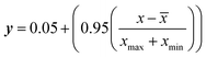
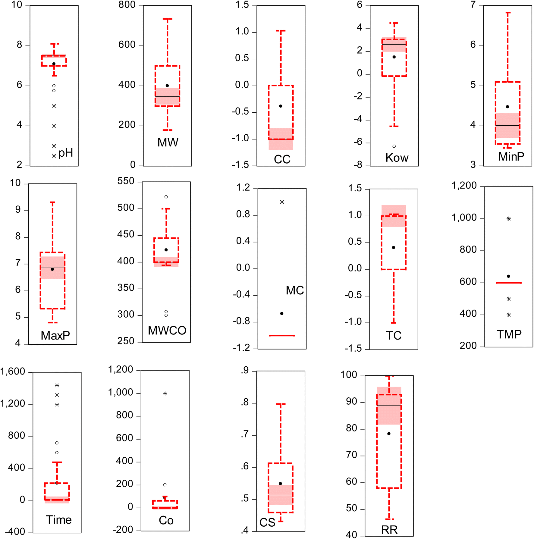
Despite the significant advancements in AI-driven models, they are limited by issues such as underfitting or overfitting, which significantly hinder the model's performance. Overfitting impairs the model's ability to generalize beyond the training data, leading to discrepancies between training outcomes and validation performance. It is imperative to employ rigorous validation techniques to enhance model robustness and reliability. In line with the findings of several researchers, both internal and external validations are crucial during the model development process to ensure the models' applicability to unseen data. This research highlights the effectiveness of k-fold cross-validation in assessing the models' performance across various scenarios. Moreover, alternative validation methodologies such as the leave-one-out, holdout, and others have been effectively implemented, as demonstrated by recent studies. It is worth mentioning that noise in this context refers to any irrelevant or extraneous data points that could distort the model's predictive accuracy. This includes measurement errors, inconsistencies in data sources, and outliers that do not follow the general trend of the dataset. The study employed human-inspection and statistical visualization to identify noise. For instance, outlier detection methods such as the box-whisker analysis were used to pinpoint irregular near and far outliers' data points (Fig. 1). Furthermore, domain-specific knowledge was applied to identify and remove data points that were deemed inconsistent with expected membrane performance metrics. Similarly, redundant elimination data points, such as duplicate entries or highly correlated variables, were checked, identified, and removed.
 |
| | Fig. 1 Box-whisker analysis of output and input variables. | |
Proposed methodology
Linear regression (LR)
LR is a statistical technique used to model the relationship between a dependent variable and one or more independent variables using a linear equation applied to observed data. The micropollutant removal efficiency is represented by the dependent variable (y), while the independent variables (x) function as predictors. The regression coefficients (β) function as weights for x, representing micropollutant properties, membrane properties, and experimental conditions. They signify the anticipated variation in y, which denotes micropollutant removal efficiency, in response to a unit change in x while holding other variables constant.where ε is the error function. LR relies on four critical assumptions: the presence of a linear relationship between the dependent and independent variables, independence of observations, homoscedasticity, and normal distribution of error terms, which ensures the reliability of statistical inferences.37 LR is commonly employed for predicting patterns, assessing the strength of predictors, and elucidating relationships between variables.
Stepwise linear regression (SLR)
SLR automates the selection of predictive variables for regression models, iteratively adding or removing variables based on their statistical significance and criteria like p-values or information criteria such as Akaike Information Criterion (AIC) or Bayesian Information Criterion (BIC). This method simplifies model building by systematically evaluating each variable's contribution and ensuring only statistically relevant predictors are included while balancing complexity and interpretability to mitigate potential overfitting. It employs forward selection, backward elimination, or hybrid approaches to dynamically adjust the model, continuously evaluating fit to ensure improvements and balance between fit and complexity. The general equation formulation for predicting micropollutant removal efficiency (y) through SLR entails constructing a linear association with a collection of independent variables (x1, x2, x3). This equation can be expressed as:| | |
y = β0 + β1x1 + β2x2 + β3x3 + ε
| (3) |
SLR relies on fundamental assumptions such as a linear relationship between dependent and independent variables, absence of perfect multicollinearity, homoscedasticity, and normally distributed errors.38 The selection criteria for variables need to accurately reflect their contribution to the model, avoiding bias or overfitting. Ultimately, SLR aims to identify a concise model that incorporates the most pertinent predictors while mitigating overfitting and ensuring both precision and conciseness in the final model.
Multivariate linear regression (MLR)
MLR is a statistical technique used to analyze the relationship between multiple independent variables and a single dependent variable. MLR relies on key assumptions such as linearity between dependent and independent variables, independence of errors, homoscedasticity ensuring consistent error variance, normality of error distribution aiding accurate estimation, and absence of multicollinearity to maintain model interpretability. The coefficients in MLR represent the relationship between each independent variable and the dependent variable, with the error term representing the discrepancy between observed and predicted values of the dependent variable.39 The goal of MLR is to minimize the sum of squared errors to produce the best-fitting model explaining the relationship between independent variables and the dependent variable, enabling analysis of intricate datasets for deeper insights into factors impacting the dependent variable. The general equation formulation for predicting micropollutant removal efficiency (y) via MLR entails creating a linear relationship with a group of independent variables (x1, x2, …, xn). This equation can be articulated as:| | |
y = β0 + β1x1 + β2x2 + β3x3…βnxn + ε
| (4) |
Support vector machine (SVM)
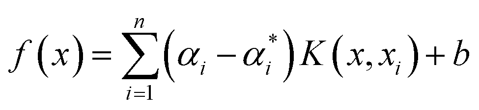
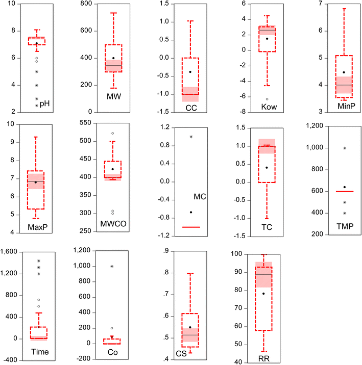
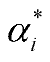
SVM models are robust supervised learning algorithms utilized for classification and regression tasks. Their operation involves identifying an optimal hyperplane to separate distinct classes within the dataset, maximizing the margin between this hyperplane and the nearest data points termed support vectors. SVMs demonstrate efficacy particularly in high-dimensional datasets, even when dimensions exceed the number of data points. Leveraging the kernel trick, SVMs adeptly address non-linear data by transforming it into higher-dimensional spaces conducive to linear separation.40 Furthermore, SVMs showcase memory efficiency by employing only a subset of training data (support vectors) for prediction. Nonetheless, they come with trade-offs, such as computational complexity in optimizing the hyperplane for sizable datasets and the necessity for careful selection of kernel functions for non-linear data, often necessitating experimentation. Scheme 1 shows the SVM model structure for micropollutant RR(%).The training set consists of the regression vector representing micropollutant properties, membrane properties, and experimental conditions in the input space (x1, x2, …, xn), along with their corresponding output space of micropollutant removal efficiency (y1, y2, …, yn).The mapping function (φx) transforms the input data into a higher-dimensional feature space, denoted as follows:41where ω and b are the weight vector and bias, respectively. The regression function associated with Lagrange multipliers (αi,  ) and the kernel function (K(x,xi)) for constrained optimization problems are expressed as follows:
| |
 | (6) |
 |
| | Scheme 1 Schematic of SVM, BT and NF model structure. | |
SVMs operate on several assumptions, including the need for scaled features to prevent dominance by any single feature and reliance on clean, representative data free from significant errors or outliers. They are primarily designed for binary classification tasks, although extensions exist for multi-class scenarios, and in the absence of a specified kernel, SVMs default to assuming a linear decision boundary.
Boosted trees (BT)
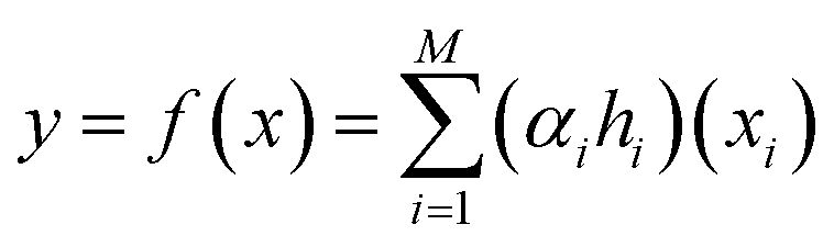
BT, also known as gradient boosting machines, amalgamate numerous weak learners, typically decision trees, to construct a robust predictive model via ensemble learning. Unlike standalone decision trees, BT iteratively generate a sequence of trees, with each subsequent tree rectifying errors from its predecessors. This iterative process emphasizes misclassified or inadequately predicted data points, diminishing model bias and bolstering overall accuracy. By amalgamating predictions from multiple trees, BT adeptly capture intricate data patterns, making them effective for regression and classification tasks. Despite their efficacy, they may be susceptible to overfitting if not finely tuned, and training may be computationally demanding compared to simpler models. Nonetheless, BT remain widely employed due to their resilience and exceptional predictive capabilities across diverse domains. The process involves sequentially fitting decision trees to the residuals of prior trees, with each tree aiming to rectify errors from its predecessors. Model representation entails aggregating these trees into a single predictive model, where each tree contributes by assigning a weight to its output. The final prediction results from combining the outputs of all trees, forming an ensemble model where each tree's contribution depends on its ability to reduce overall prediction error. The schematic of BT model structure for micropollutant RR(%) is shown in Scheme 1. The BT regression equation for predicting micropollutant removal efficiency (y) based on input variable (x) is defined by the ith weight (αi), the ith prediction (hi), and the total number of trees (M). It can be presented as follows:42| |
 | (7) |
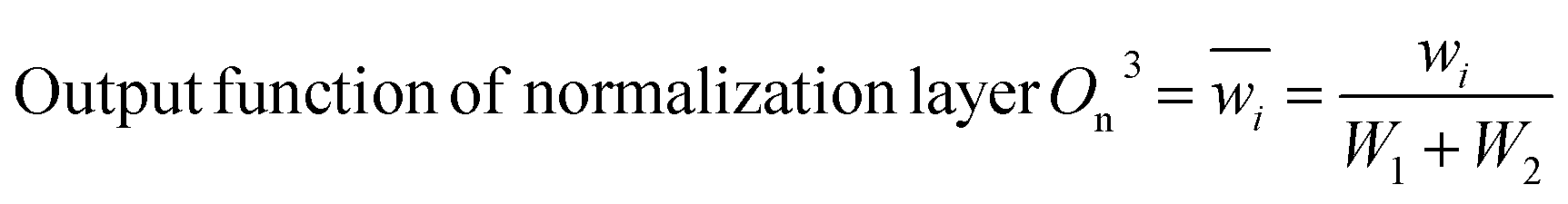
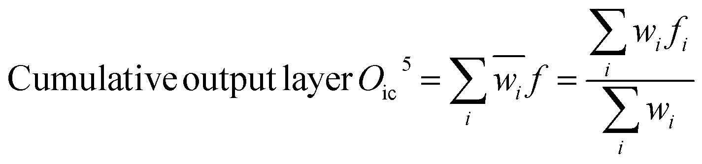
Adaptive network-based fuzzy inference system (NF)
The Neuro-Fuzzy (NF) approach combines neural networks learning capabilities with the human-like reasoning of fuzzy inference systems. In NF systems, fuzzification maps discrete inputs to fuzzy sets, followed by the application of fuzzy rules in the inference layer and defuzzification to convert fuzzy outputs to precise values.43| | |
Output function of input layer Oi1 = μAi(x)
| (8) |
| | |
Output function of fuzzification layer Of2 = wi = μAi(x) × μBi(y)
| (9) |
| |
 | (10) |
| |
 | (11) |
| |
 | (12) |
Scheme 1 shows the NF model structure for micropollutant RR(%). In the NF architecture, the backpropagation algorithm precisely adjusts the membership function parameters within the neural network layer to optimize the input-to-fuzzy-value mapping. Simultaneously, the least-squares estimation (LSE) method refines the consequent parameters of fuzzy logic rules for optimal parameter estimation in the output stage. This procedural sequence enables NF systems to efficiently adapt and fine-tune parameters, making them proficient in simulating and navigating intricate, non-linear dynamics. NF requires data to train its fuzzy membership functions and rules, with more complexity demanding more data for effective learning. It strikes a balance between interpretability and accuracy, although prioritizing interpretability may require limiting model complexity, potentially affecting accuracy.
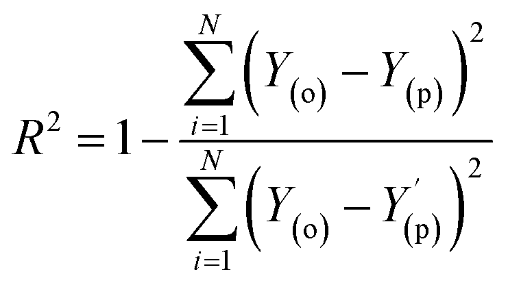
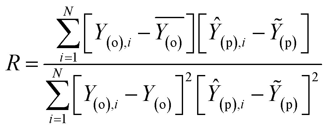
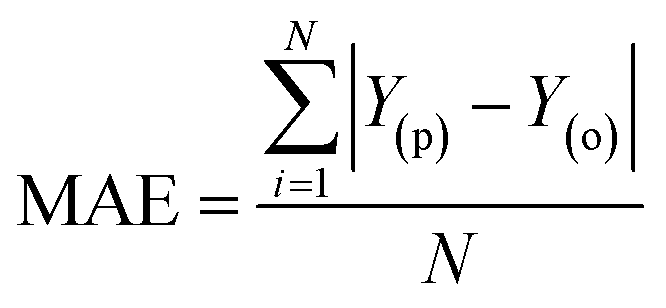
Evaluation criteria
The evaluation of ML algorithm predictive accuracy for micropollutant removal efficiency encompasses the use of various statistical and error metrics. It includes measures such as correlation coefficient (R), determination coefficient (R2), mean squared error (MSE), mean absolute error (MAE), and root mean squared error (RMSE). The metrics are computed utilizing the observed data (Y(o)), predicted Y(p) dataset with a total number of data points (N). They are expressed through the following equations.| |
 | (13) |
| |
 | (14) |
| |
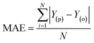 | (15) |
| |
 | (16) |
| |
 | (17) |
Results and discussion
In this study, the models such as NF-GP, NF-SC SVM, BT, LR, and SLR were implemented using the MATLAB 2023b (R2023b) predictive toolbox while the MVR was used in Microsoft Data toolbox. Similar to other data-driven algorithms, the optimal parameters for NF, SVM, and BT were identified through a series of trial-and-error methods. These methods involve hyper-parameter tuning and evaluating the model's performance to find the best combination. The models were initially calibrated using the training data to ensure they could accurately learn the underlying patterns. Once calibrated, the trained models were applied to the testing data to validate their predictive capabilities and to fine-tune the parameters further. For the NF modeling, we explored different types of membership functions (MFs) through an iterative trial and error process. This involved testing various MF types and adjusting epoch iterations to find the best configuration for the NF model. Each structure's performance was assessed to ensure that the chosen configuration provided the most accurate predictions. For the SVM models, we investigated different structural configurations for all possible input combinations. To achieve the highest accuracy in the SVM models, it was essential to determine the optimal values for the C and g parameters, which control the trade-off between achieving a low training error and a low testing error, and the kernel's influence, respectively. We employed the grid search method, a systematic approach that involves searching through a manually specified subset of the hyperparameter space of the learning algorithm, to identify the optimal parameter values. This comprehensive approach to parameter tuning, involving trial and error for NF and grid search for SVM, ensures that the models are robust, accurate, and well-suited to the data. Each step, from model calibration to parameter optimization, is crucial in developing predictive models that can generalize well to unseen data, providing reliable and accurate predictions. The procedure was applied to other employed models employed in this study.
The predictive ML algorithm analysis of micropollutant rejection rate involves the feature selection and data distribution examination across 14 input variables and 6 model configurations. Additionally, it involves evaluating the predictive performance of 7 ML algorithms and comparing the superior algorithm's effectiveness in prediction. The perfect model demonstrates the highest prediction accuracy while exhibiting minimal error metrics. Comprehending the impact of dataset features and model architecture on predictive performance is crucial for a thorough evaluation in ML algorithm. Table 2 shows the accuracy and error metrics of predictive NF-GP, NF-SC, LR, SLR, MVR, SVM and BT ML algorithm on micropollutant removal rate. Sparse dataset modeling is greatly affected by variations in distributions, noise levels, and patterns, as well as differences in model complexity, assumptions, and algorithms. Feature selection is crucial for enhancing prediction accuracy in small datasets, as informative features are meticulously chosen to mitigate noise and prioritize impactful variables, improving model performance despite data scarcity challenges. A convenient and effective modeling strategy of feature selection combined ML algorithm approach for the efficient predicting micropollutant removal rates.
Table 2 Evaluating statistical indicators and error metrics for ML algorithms predicting micropollutant rejection rates (%)
| Models |
Calibration phase |
Verification phase |
| R2 |
R |
MSE |
RMSE |
MAE |
R2 |
R |
MSE |
RMSE |
MAE |
| NF-GP-C1 |
0.916 |
0.957 |
31.563 |
5.618 |
0.544 |
0.649 |
0.806 |
27.522 |
5.246 |
0.544 |
| NF-SC-C1 |
0.950 |
0.975 |
18.860 |
4.343 |
0.044 |
0.872 |
0.934 |
10.003 |
3.163 |
0.044 |
| NF-GP-C2 |
0.932 |
0.965 |
25.754 |
5.075 |
0.003 |
0.731 |
0.855 |
21.119 |
4.596 |
0.003 |
| NF-SC-C2 |
0.945 |
0.972 |
20.950 |
4.577 |
0.259 |
0.766 |
0.875 |
18.372 |
4.286 |
0.259 |
| NF-GP-C3 |
0.229 |
0.479 |
291.074 |
17.061 |
0.434 |
0.825 |
0.909 |
13.683 |
3.699 |
0.434 |
| NF-SC-C3 |
0.225 |
0.475 |
292.514 |
17.103 |
0.499 |
0.842 |
0.917 |
12.406 |
3.522 |
0.499 |
| NF-GP-C4 |
0.932 |
0.965 |
25.664 |
5.066 |
0.703 |
0.667 |
0.817 |
26.126 |
5.111 |
0.703 |
| NF-SC-C4 |
0.947 |
0.973 |
19.850 |
4.455 |
0.561 |
0.673 |
0.820 |
25.656 |
5.065 |
0.558 |
| NF-GP-C5 |
0.965 |
0.982 |
13.328 |
3.651 |
0.217 |
0.910 |
0.954 |
7.041 |
2.653 |
0.217 |
| NF-SC-C5 |
0.965 |
0.982 |
13.398 |
3.660 |
0.193 |
0.910 |
0.954 |
7.089 |
2.663 |
0.193 |
| NF-GP-C6 |
0.219 |
0.468 |
295.070 |
17.178 |
0.581 |
0.639 |
0.799 |
28.329 |
5.323 |
0.581 |
| NF-SC-C6 |
0.227 |
0.477 |
291.898 |
17.085 |
0.497 |
0.860 |
0.927 |
10.988 |
3.315 |
0.526 |
| LR-C1 |
0.612 |
0.783 |
146.418 |
12.100 |
1.630 |
0.553 |
0.744 |
92.958 |
9.641 |
1.630 |
| LR-C2 |
0.470 |
0.686 |
199.983 |
14.142 |
0.325 |
0.342 |
0.585 |
97.386 |
9.868 |
0.325 |
| LR-C3 |
0.130 |
0.361 |
328.574 |
18.127 |
1.493 |
0.132 |
0.364 |
68.047 |
8.249 |
1.493 |
| LR-C4 |
0.215 |
0.464 |
296.303 |
17.213 |
3.659 |
0.437 |
0.661 |
123.578 |
11.117 |
3.659 |
| LR-C5 |
0.940 |
0.970 |
22.507 |
4.744 |
0.005 |
0.762 |
0.873 |
18.637 |
4.317 |
0.005 |
| LR-C6 |
0.171 |
0.413 |
313.242 |
17.699 |
0.828 |
0.287 |
0.535 |
40.273 |
6.346 |
0.828 |
| SLR-C1 |
0.833 |
0.913 |
63.028 |
7.939 |
1.134 |
0.751 |
0.867 |
47.636 |
6.902 |
1.134 |
| SLR-C2 |
0.939 |
0.969 |
23.204 |
4.817 |
0.198 |
0.739 |
0.860 |
20.471 |
4.525 |
0.198 |
| SLR-C3 |
0.133 |
0.365 |
327.443 |
18.095 |
2.039 |
0.105 |
0.324 |
78.485 |
8.859 |
2.039 |
| SLR-C4 |
0.137 |
0.371 |
386.269 |
19.654 |
2.933 |
0.126 |
0.355 |
98.966 |
9.948 |
2.933 |
| SLR-C5 |
0.929 |
0.964 |
26.810 |
5.178 |
0.613 |
0.711 |
0.843 |
22.631 |
4.757 |
0.613 |
| SLR-C6 |
0.133 |
0.365 |
327.443 |
18.095 |
2.039 |
0.148 |
0.385 |
78.485 |
8.859 |
2.039 |
| MVR-C1 |
0.636 |
0.797 |
137.621 |
11.731 |
1.262 |
0.567 |
0.753 |
91.499 |
9.566 |
1.262 |
| MVR-C2 |
0.494 |
0.703 |
190.981 |
13.820 |
0.097 |
0.337 |
0.580 |
97.733 |
9.886 |
0.097 |
| MVR-C3 |
0.186 |
0.431 |
307.358 |
17.532 |
1.591 |
0.182 |
0.426 |
64.163 |
8.010 |
1.591 |
| MVR-C4 |
0.220 |
0.469 |
294.653 |
17.165 |
3.705 |
0.188 |
0.434 |
122.460 |
11.066 |
3.705 |
| MVR-C5 |
0.735 |
0.857 |
100.156 |
10.008 |
0.993 |
0.563 |
0.750 |
104.227 |
10.209 |
0.993 |
| MVR-C6 |
0.165 |
0.407 |
315.239 |
17.755 |
2.243 |
0.142 |
0.377 |
78.081 |
8.836 |
2.243 |
| SVM-C1 |
0.856 |
0.925 |
54.459 |
7.380 |
0.458 |
0.696 |
0.834 |
23.830 |
4.882 |
0.585 |
| SVM-C2 |
0.923 |
0.961 |
29.220 |
5.406 |
0.201 |
0.726 |
0.852 |
21.521 |
4.639 |
0.281 |
| SVM-C3 |
0.157 |
0.397 |
474.849 |
21.791 |
10.545 |
0.135 |
0.367 |
67.833 |
8.236 |
0.850 |
| SVM-C4 |
0.914 |
0.956 |
32.633 |
5.713 |
1.291 |
0.648 |
0.805 |
27.572 |
5.251 |
0.259 |
| SVM-C5 |
0.919 |
0.959 |
30.609 |
5.533 |
0.166 |
0.745 |
0.863 |
20.008 |
4.473 |
0.542 |
| SVM-C6 |
0.156 |
0.395 |
459.096 |
21.427 |
11.289 |
0.270 |
0.520 |
57.216 |
7.564 |
0.787 |
| BT-C1 |
0.901 |
0.949 |
37.470 |
6.121 |
3.422 |
0.659 |
0.812 |
26.768 |
5.174 |
1.284 |
| BT-C2 |
0.907 |
0.952 |
35.291 |
5.941 |
2.824 |
0.654 |
0.808 |
27.163 |
5.212 |
1.882 |
| BT-C3 |
0.175 |
0.418 |
311.623 |
17.653 |
2.480 |
0.205 |
0.452 |
51.297 |
7.162 |
2.227 |
| BT-C4 |
0.880 |
0.938 |
45.240 |
6.726 |
2.499 |
0.577 |
0.759 |
48.869 |
6.991 |
2.208 |
| BT-C5 |
0.909 |
0.954 |
34.295 |
5.856 |
3.106 |
0.772 |
0.879 |
17.891 |
4.230 |
1.600 |
| BT-C6 |
0.169 |
0.411 |
313.848 |
17.716 |
2.573 |
0.135 |
0.367 |
50.927 |
7.136 |
2.133 |
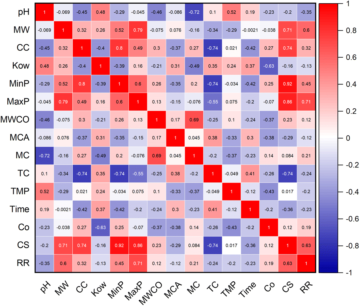
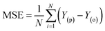
Analysis of feature selection and data distribution
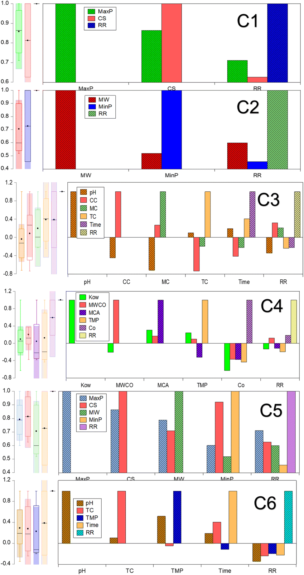
The proposed ML algorithm tools were aimed to evaluate the impact of various input variables, such as properties of micropollutant, membrane specifications, and experimental parameters, precisely predicting the target variable as removal rate (RR) (%). The chosen 14 input variables are properties of micropollutant (pH, MW, CC, Kow, CS, MinP, and MaxP), functionalized membrane (MWCO, MCA, MC, TC) and experimental parameters (TMP, T and C0). The deployed ML tools are NF, LR, SLR, MVR, SVM and BT. Fig. 2 shows the parametric dependency analysis between the 14 input variables and rate of micropollutant removal. The model configurations are classified according to the hierarchical value of the correlation between the input variable and the targeted micropollutant removal rate (%). It is important to note that model selection is a crucial step in building a predictive model, as it ensures that the selected features significantly contribute to the accuracy and reliability of the predictions. By carefully analyzing the dependency between various variables and the target variable (RR), we can identify and prioritize those that have the most substantial impact. The study approach involved categorizing the variables into different classes (C1 to C6) based on their correlation strength with RR. For instance, C1 (MaxP, CS, RR), C2 (MW, MinP, RR), C3 (pH, CC, MC, TC, Time, RR), C4 (Kow, MWCO, MCA, TMP, Co, RR), C5 (MaxP, CS, MW, MinP, RR), C6 (pH, TC, TMP, Time, RR). In C1, we used variables with strong direct positive correlations with RR, ranging between 60–80%, such as CS (0.626), MaxP (0.711), and MW (0.599). For C2, we selected moderate direct positive variables with correlations ranging between 20-40%, including MinP (0.455) and Co (0.186). C3 included both direct and indirect variables with correlations between 50-60%, such as CC (0.317) and MC (0.208). In C4, we considered both direct and indirect variables with correlations ranging between 10-20%, including MCA (−0.118), TMP (−0.199), and time (−0.226). For C5, we focused on the strongest positive variables overall, ensuring they significantly impact the prediction, such as CS and MaxP. Finally, in C6, we included the strongest negative variables to understand their adverse impact on RR, such as pH (−0.346) and TC (−0.243). This systematic and detailed approach to model selection ensures that our predictive model for rejection rate (RR) is robust, reliable, and highly accurate (Fig. 2). The reasons behind the specific parameter choices for our model selection are established in their dependency strengths with the target variable (RR) and their potential impact on the model's predictive power. The study included parameters with strong direct positive correlations because they significantly improve rejection rate predictions. Moderate direct positive variables were selected for their positive but less significant contributions. Both direct and indirect variables help capture the relationship between compound characteristics and rejection rate. Similarly, the variables with smaller correlations for a comprehensive model. The strongest positive variables were chosen for their consistently high correlations with RR. Furthermore, this study also considered the strongest negative variables to understand their adverse impacts on RR. This systematic approach ensures that our predictive model for RR is robust, reliable, and highly accurate.
 |
| | Fig. 2 Correlation analysis of input variables on micropollutant rejection rate. | |
As seen in Fig. 3, MaxP demonstrated a robust correlation, quantified as 0.711, with the removal rate (%) of micropollutants, specifically under the model configuration (C1) that accounted for the highest influence, spanning from 70% to 60%. Table 3 shows the statistical features of data distribution of input and out variables. The additional significant variable, CS, displayed a low standard deviation (SD) of 0.109, with its data extending from 0.438 to 0.798 Å. For the configuration C2, where the correlation of input variables like MinP and MW ranged between 40–50%, Mw displayed the highest correlation with the rejection rate (%). The distribution of Mw data ranged from 179 to 733 g mol−1, exhibiting a higher SD and modest skewness value of 145.495 and 0.969, respectively. The correlation and feature engineering indicated that the micropollutant properties such as MaxP, MinP, MW and CS are significant control in the RO and NF membranes. This mechanism was due to the MW and CS are dominant in the size exclusion phenomena and other MaxP and MinP corresponds to the adsorption of micropollutant on the membrane surface. The effectiveness of size exclusion in filtering micropollutants is largely determined by their MW and CS, which dictate the retention of micropollutant in low pore size NF and RO membranes. In contrast, the adsorption process, where micropollutants bind to the membrane surface, is significantly influenced by their MaxP and potentially MinP, highlighting the physical properties impact the separation process. The subsequent configuration, C3, incorporates variables such as pH, CC, MC, TC, and time interval, which all fall within a 20–30% correlation range with respect to the targeted removal rate percentage. pH, T and TC had inverse relationship with micropollutant rejection rate (%). Within the input variables of configuration C3, the range between the maximum and minimum values is notably wider for the T, covering from 1440 to 10 minutes. The distribution of MC and TC data closely aligned within the range of −1 to 1.032, with a lower skewness observed for both pH and TC. It was crucial to note that key parameters, including Kow, MWCO, MCA, TMP, and C0, exhibited minimal correlation dependency, ranging from 10–20%, with the target dataset within the C4 combination. The TMP showed the greatest standard deviation, recorded at 169.586, and an inverse correlation with the targeted output response was noted for TMP, along with Kow and MCA. These combinations suggest that the datasets are intricate, displaying complex and non-linear correlations with the micropollutant rejection rate (%). Therefore, meticulous attention is required in the selection of input variables for effective modeling to prevent data leakage. Consequently, the four foremost input variables demonstrating either positive or negative correlations were systematically segregated into two distinct groups, combinations C5 and C6. This stratification was executed to scrutinize their respective influences on the accuracy of predicting the targeted response for micropollutant removal. The four primary input variables exhibiting significant positive correlations in combination C5 include MaxP, MinP, MW, and CS. It revealed that the micropollutant properties such as MaxP, MinP, MW, and CS are meticulously considered into account for the real-time filtration application. This study also enables the design of self-fabricated membranes with optimized pore sizes for improved separation of micropollutants from wastewater.
 |
| | Fig. 3 Parametric dependency analysis of input variables on micropollutant rejection rate. | |
Table 3 Impact of descriptive statistics and subset data of input variables for micropollutant removal rate
| Variables |
Mean |
SD |
Skewness |
Minimum |
Maximum |
Subset data |
| pH |
7.09 |
1.12 |
−2.42 |
2.5 |
8.1 |
Experimental data source,24 total data instances: 990, data characteristics: 15 variables (14 inputs and 1 output), type of membrane: dual layer hollow fiber TFC membrane,31 crosslinked cellulose TFC membrane,32 poly(piperazine-amide) TFC membrane,33 ceramic NF membrane,34 imidazolium ionic liquid plugged poly(piperazine-amide) TFC membrane35 and zwitterionic poly(amino piperazine-amide) membrane36 |
| MW |
400.15 |
145.5 |
0.97 |
179.22 |
733.94 |
| CC |
−0.38 |
0.76 |
0.77 |
−1 |
1.03 |
| Kow |
1.5 |
2.86 |
−0.98 |
−6.3 |
4.49 |
| MinP |
4.47 |
1.09 |
1 |
3.45 |
6.83 |
| MaxP |
6.8 |
1.36 |
0.33 |
4.81 |
9.32 |
| MWCO |
422.84 |
49.94 |
−0.24 |
300 |
522 |
| MCA |
40.79 |
9.05 |
−0.83 |
11 |
65.9 |
| MC |
−0.67 |
0.75 |
1.86 |
−1 |
1 |
| TC |
0.41 |
0.75 |
−0.83 |
−1 |
1.03 |
| TMP |
639.34 |
169.59 |
1.41 |
400 |
1000 |
| Time |
218.52 |
412.33 |
2.02 |
10 |
1440 |
| Co |
86.92 |
219.44 |
3.7 |
0.02 |
1000 |
| CS |
0.55 |
0.11 |
1.05 |
0.43 |
0.8 |
| RR |
78.26 |
18.65 |
−0.61 |
46.33 |
100 |
Performance evaluation of predictive ML algorithm: error metrics and accuracy
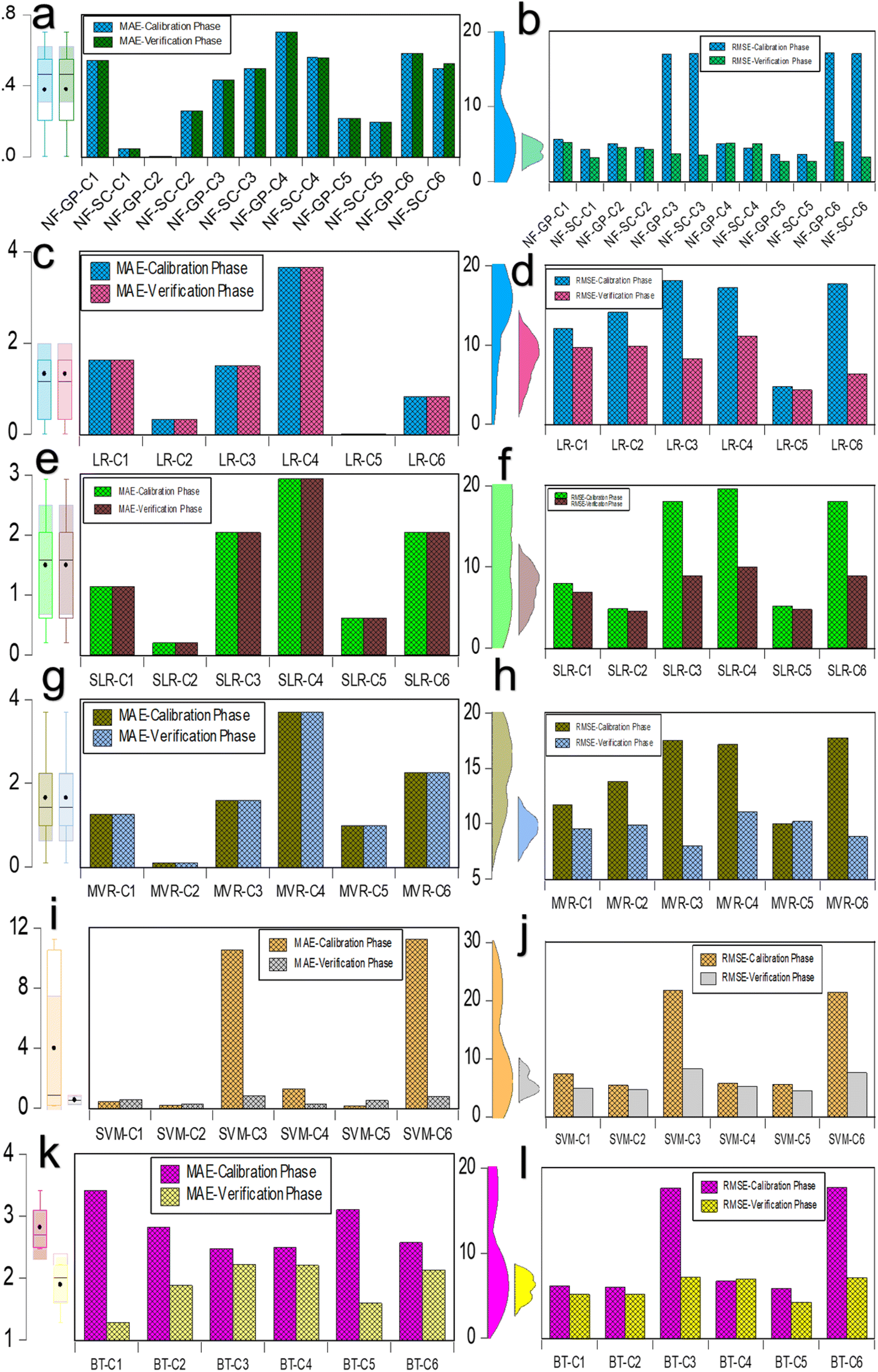
Fig. 4 illustrates the comparative analysis of MAE and RSME data for the predictive NF, LR, SLR, MVR, SVM and BT models evaluated on calibration and verification datasets for combinations C1 through C6. As seen in Fig. 4a and b, MAE does not have much deviation in both the NF grid partition (NF-GP) and subtractive clustering (NF-SC) for the combination C1 to C6. It indicated that both grid partition (GP) and subtractive clustering (SC) methods held similarly minor prediction errors of micropollutant removal rate (%). Among the combination in NF, NF-GP-C4 exhibit highest MAE value (0.703) and predominant with NF-GP-C1 (0.544), NF-SC-C4 (0.561), and NF-GP-C6 (0.860). In RMSE, the deviation was observed in data mining and segmentation strategies of GP and SC notably in the C3 and C6. The deviation in verification and calibration phase was due to the data distribution and descriptive statistics. In GP, the dataset is segmented into a uniform grid of hypercubes, leading to variations in data distribution representation. Conversely, SC delineates clusters based on the density of data points, yielding enhanced distinctions and more precise predictive outcomes. GP divides the data space into a grid of hypercubes, assigning data points to these cubes, which can lead to a uniform treatment of the data space regardless of the density of points. This method may not always capture the nuances in data distribution, potentially affecting the precision of predictions and, consequently, the MAE and RMSE values. In contrast, SC identifies cluster centers based on the density of data points, which can result in a more nuanced and potentially more accurate modeling of data relationships, impacting the MAE and RMSE values differently. Another, RMSE confines the identification of large errors in the predictive model dataset. The NF-GP-C5 and NF-SC-C5 exhibited notably lower MAE values of 0.217 and 0.193, respectively, accompanied by minimal RMSE values of 3.651 and 3.660. In comparison to neural fuzzy models, the MAE and RMSE values were higher in LR frameworks across all the combinations except C5. It was imperative to observe that MAE has no deviation in both calibration and verification phase for the LR framework of LR, SLR and MLR (Fig. 4c–h). In LR framework (LR, SLR and MLR), C4 displayed the maximum MAE value owed to the predictive rejection rate (%) for the input variables (Kow, MWCO, MCA, TMP and Co). Combination C4 emerged from a correlation significance range of 10–20% among input variables, indicating a relatively minor impact. This pattern of LR approaches had good agreement with above NF-GP model. The other combination ranking based on MAE varied with one another in LR approaches. The observed pattern can be attributed to the fact that LR relies on assumption of linearity between variables, SLR operates through an automated process of iterative forward selection and backward elimination and MLR characterized by its reliance on multiple dependent variables. In evaluating regression models, the lowest MAE of 0.005 was found in the model LR-C5. However, this model also exhibited a high RMSE of 4.744, indicating the influence of outliers or significant errors. Generally, MAE values exceeded one across most configurations in LR, SLR, and MLR, suggesting suboptimal performance in these models. Moreover, the RSME value showed significant deviation in the verification and calibration phase in LR approaches (LR, SLR and MLR). The discrepancy in RMSE and MAE metrics across verification and calibration datasets underscores the predictive model's challenges in generalizing to unseen data and adapting to variations in data distribution. RMSE exhibits heightened sensitivity to substantial errors, a result of its methodology of squaring the deviations between predicted and actual values prior to averaging them. This sensitivity enabled the identification of significantly divergent values are exist in the testing dataset. Compared to LR frameworks, SVM exhibited lower MAE and RMSE values for all combinations except for C3, which had MAE and RMSE values of 10.545 and 21.791, respectively, and C6, which had values of 11.289 and 21.427, during the verification phase (Fig. 4i and j). The minimal error metric was due to the SVM utilizing the kernel function and its parameters to identify the optimal hyperplane that separates different classes in the feature space. The regularization term critically influences the attainment of an optimal solution through error minimization, harmonizing the model's intricacy with its capacity to generalize across unseen data. In BT model, calibration shower higher MAE than calibration across all combinations (Fig. 4k and l). It revealed that during the calibration phase, the BT model was not adequately refined and instead became overly tailored to the specifics of the training data, leading to a decrease in its ability to data generalization. Among the combinations, C5 displayed an advantageous result in both MAE and RMSE across each distinct model, including NF-GP-C5, NF-SC-C5, LR-C5, MVR-C5, and BT-C5. The combination C5 positively correlates with input variables including MaxP, CS, MW and MinP. This study also indicates that data splitting and data leaking have potential effect with combinations. The error metrics of the predictive model indicated model combinations had wider influence in data generalization and optimal solution for prediction accuracy. This independent model examination unequivocally demonstrates the complexity inherent within the datasets, highlighting the specific combinations significantly influence the error metrics associated with predicting micropollutant rejection rates.
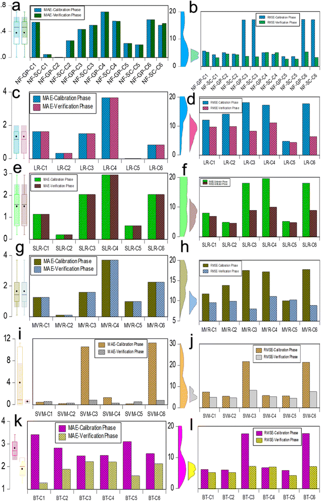 |
| | Fig. 4 Comparison of MAE and RMSE data for predictive ML models assessed on calibration and verification datasets across six combinations. (a and b) MAE and RMSE assessments for the NF-GP and NF-SC models prediction; (c and d) MAE and RMSE for the LR model predictions; (e and f) MAE and RMSE for the SLR model predictions; (g and h) MAE and RMSE for the MVR model predictions; (i and j) MAE and RMSE for the SVM model predictions; and (k and l) MAE and RMSE for the BT model predictions during both calibration and verification phases. | |
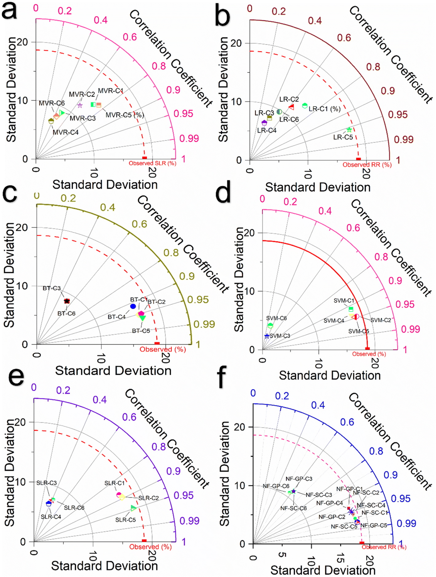
Fig. 5 presents a comparison using a Taylor plot of the correlation coefficients (R) for various predictive models including NF-GP, NF-SC, LR, SLR, MVR, SVM and BT across six combination C1 to C6. As seen in Fig. 5f, NF-GP and NF-SC models showed a linear relationship with superior correlation coefficient for the C1, C2, C4 and C5. For the C5 combination, both the NF-GP and NF-SC models achieved R of 0.982, indicating a very high degree of linear correlation between predicted and observed values. However, the performance was lower in the C6. The reduced linear correlation for C3 and C6 in the GP and SC models suggests a limitation within these models to discern the intricate patterns in the input variables of C3 (pH, CC, MC, and TC) and C6 (pH, CC, TMP, and time). Among a total of 12 model combinations evaluated in NF, 8 displayed a close linear relationship in comparison with the NF-GP and NF-SC models. The enhancement in correlation coefficient can be attributed to the GP model's efficient organization of the dataset, focusing on localized patterns within individual grid cells, alongside the SC model's precise identification of cluster centers through subtractive clustering. It reveals a potential challenge in effectively modeling the complexity inherent in these specific pH and TC combinations. For the C5 combination, both the NF-GP and NF-SC models achieved R of 0.982, indicating a very high degree of linear correlation between predicted and observed values. However, the performance was lower in the C6. A similar pattern was noted, though with slightly decreased correlation coefficients, in both the SVM and BT models Fig. 5c and d. The SVM excels in classification and regression tasks within high-dimensional contexts, adeptly managing complex input variables even when features outnumber samples. In the SVM model, the C5 combination showed a strong R of 0.959 with lower error metrics than other combinations in both verification and calibration phase, indicating efficient predictive accuracy. This makes SVM highly effective for elucidating the complex dynamics between input variables and micropollutant removal rates. Meanwhile, BT stand out for their capacity to reduce bias and variance, enhancing predictive precision, notably in linking complex inputs to micropollutant removal efficiency. C5 combination achieved a correlation coefficient (R) of 0.954, indicating a very high degree of linear correlation between the predicted and observed values in BT model. In the LR framework, models demonstrated linear correlations with the data combinations of C1, C2, and C5. The improved outcomes can be attributed to the distinct capabilities of each modeling approach: LR accurately depicted the dependent variable's variation via linear correlations with independent variables (Fig. 5b). SLR pinpointed critical subset of predictors affecting the dependent variable (Fig. 5e). In contrast, MLR comprehensively explored the dependent variable's linear relationships by including several independent variables (Fig. 5a). Among the LR framework, the L5-C5 combination showed the highest R (0.970), indicating strong predictive performance, followed by SLR-C2 (0.969). Conversely, MVR-C5 displayed a lower R value of 0.857. Other combinations, specifically C3 and C6, also exhibited lower R values, suggesting weaker predictive capabilities.
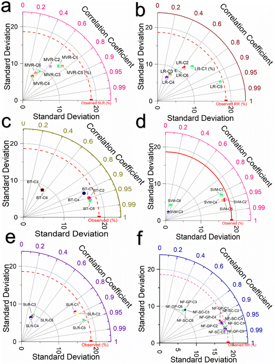 |
| | Fig. 5 Taylor plot illustrating the correlation coefficients (R) for different predictive ML models across six combinations. (a) R evaluation for the MVR model prediction; (b) R for the LR model predictions; (c) R for the BT model predictions; (d) R for the SVM model predictions; (e) R for the SLR model predictions; and (f) R for the NF-GP and NF-SC models predictions. | |
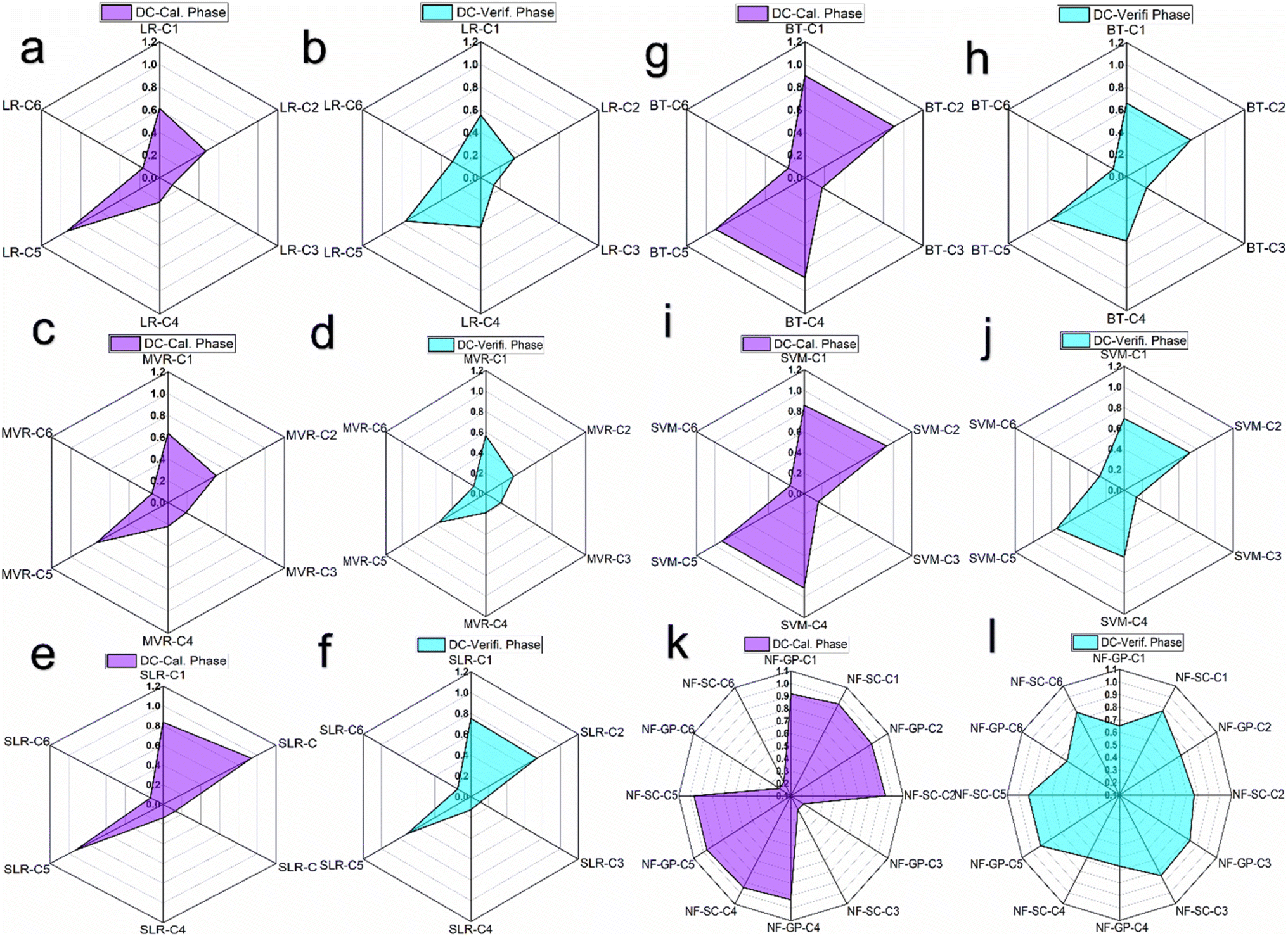
Fig. 6 presents a radar chart depicting the coefficient of determination (R2) for a range of predictive models including NF-GP, NF-SC, LR, SLR, MVR, SVM and BT evaluated across six distinct combinations C1 to C6. As seen in Fig. 6(a–f), a consistent pattern of lesser R2 value dispersion was observed for the LR paradigm of LR, SLR and MVR across data combinations C1 to C6. Among the combinations, C5 exhibited an enhanced coefficient of determination (R2) of 0.94, 0.93 and 0.74 in the LR models of LR, SLR and MVR, respectively. The diminished R2 values observed for other combinations may result from the intrinsic linear assumption within regression models (LR, SLR and MVR), which might prove inadequate for datasets characterized by complex, multidimensional constructs, and substantial data variability. Consequently, this limitation can impede the effective detection of the underlying patterns within the data. Enhanced predictive accuracy was noted for SVM and BT models in configurations C1, C2, C4, and C5, with R-squared values ranging from 0.856 to 0.923 for SVM and 0.880 to 0.909 for BT (Fig. 6(g–j)). The enhanced predictive accuracy of SVM and BT models, in comparison to conventional LR framework (LR, SLR and MVR), is primarily due to their ability to model non-linear relationships. SVM achieves this through the application of kernel functions, allowing for the accommodation of non-linear data patterns, while BT, leveraging its ensemble learning approach, significantly improves data generalization. Another reason is SVM and BT model incorporate strategies to mitigate overfitting; SVM utilizes regularization parameters to refine the margins, whereas BT employs boosting and bagging techniques to regulate tree depth. It was imperative to observe that NF models demonstrated significantly improved prediction accuracy relative to other models for combinations C1, C2, C4, and C5 (Fig. 6k and l). The R-squared value of 0.965 for both NF-GP-C5 and NF-SC-C5 indicates a high predictive accuracy, with these models explaining a substantial proportion of the variance in the dependent variable. The improved prediction accuracy was due to the intrinsic structure of NF models is specifically designed to address data uncertainty, utilizing the adjustment of fuzzy rules and membership functions to achieve a higher degree of model flexibility. Through employing grid partitioning and subtractive clustering, NF models excel in the reduction of dimensionality, effectively isolating vital clusters in smaller datasets. The lower R2 for the C6 combination across all ML models indicate that these models were less effective at explaining the variance in this configuration.
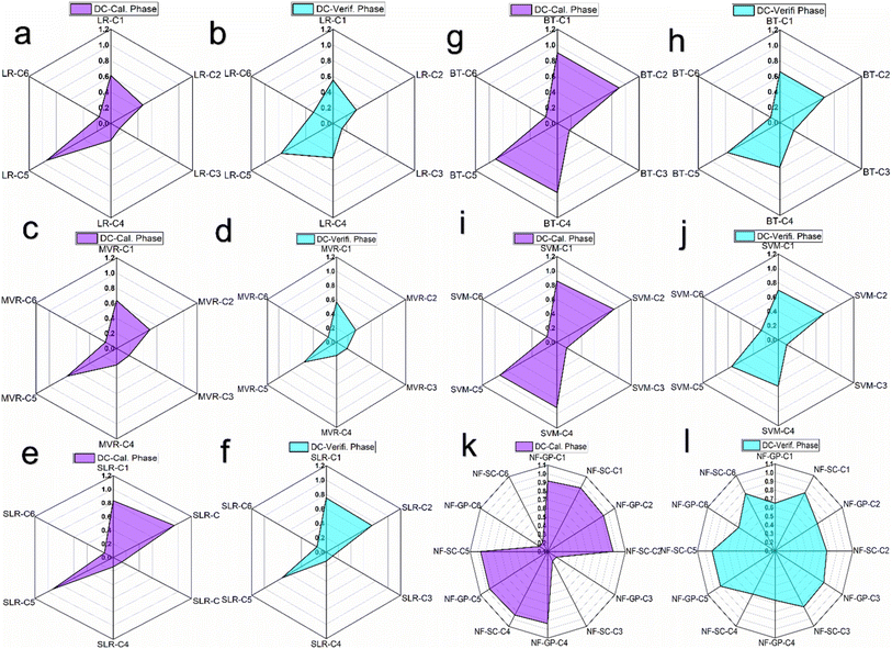 |
| | Fig. 6 Radar chart illustrating the comparison of coefficient of determination (R2) across six distinct combinations for various predictive models. (a and b) R2 assessments for the LR model prediction; (c and d) R2 for the MVR model predictions; (e and f) R2 for the SLR model predictions; (g and h) R2 for the BT model predictions; (i and j) R2 for the SVM model predictions; and (k and l) R2 for the NF-GP and NF-SC models prediction predictions during both calibration and verification phases. | |
Comparative analysis of predictive ML algorithm
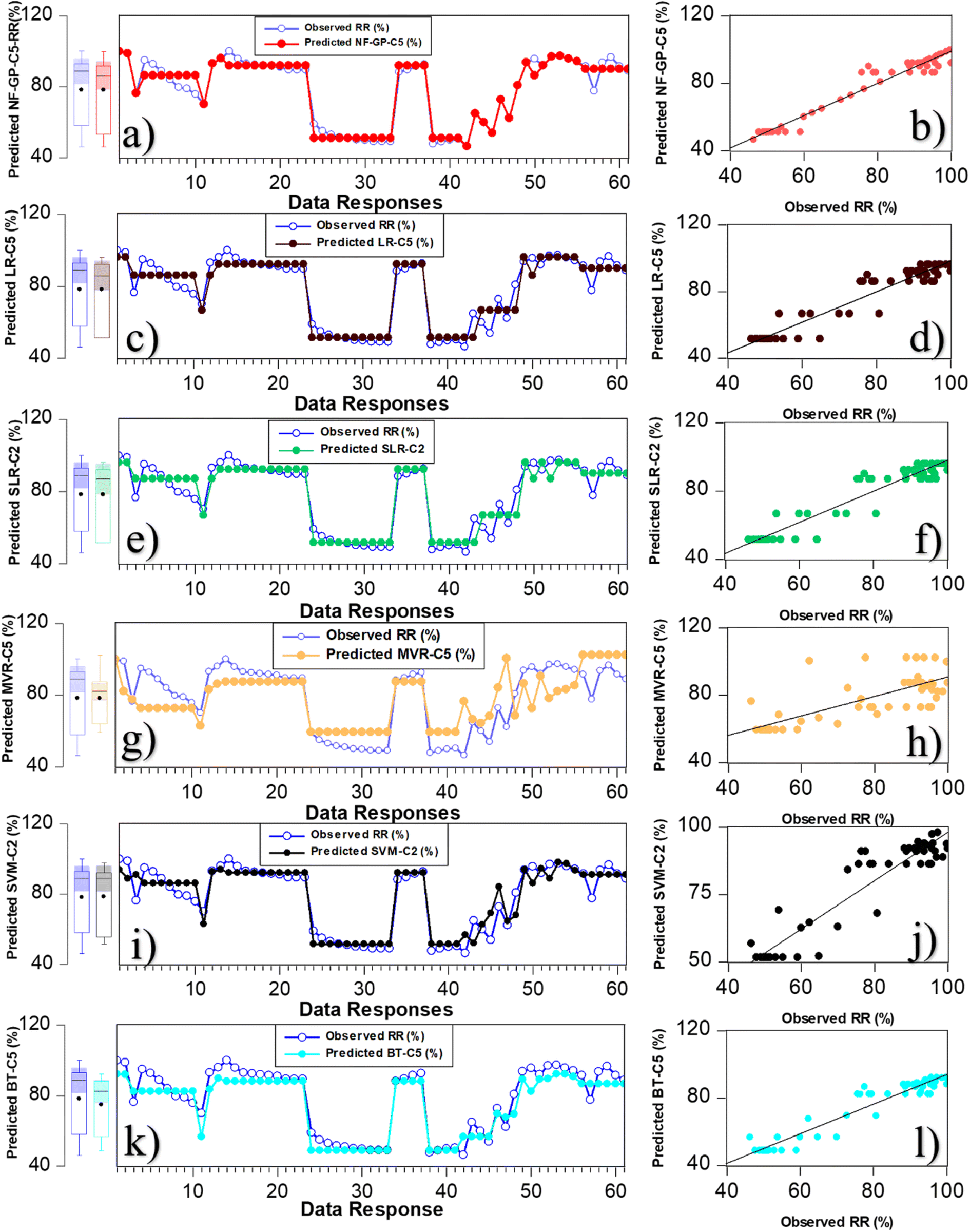
Fig. 7 shows the comparison of micropollutant rejection rate (%) data response and scatter plot for the superior predictive model of NF-GP-C5, LR-C5, SLR-C2, MVR-C5, SVM-C2 and BT-C5. From Fig. 7(a and b), the predictive model NF-GP-C5 demonstrated a high degree of fit in the data response plot, achieving an optimal R-squared (R2) value of 0.965 for the prediction of micropollutant rejection rate (%) under calibration phase. The scatter plot further substantiates this observation, with data points uniformly distributed along the line of agreement between observed and predicted values, underscoring the model's predictive precision. Similarly, the predictive models LR-C5 and SLR-C2 demonstrated a good level of agreement with the experimental data, as evidenced by their data response and scatter plot analyses (Fig. 7c–f). In the LR approaches, the models LR-C5, SLR-C2, and MVR-5 exhibited R-squared (R2) values of 0.940, 0.939, and 0.735, respectively. LR-C5 and SLR-C2 indicated that the model had linear correlation with the input variables of combination C5 and C2, respectively. The enhanced R2 metrics in LR and SLR are attributable to their focus on maintaining simplicity and clarity within the model framework, consequently leading to improvements in the precision of predictions. The SVM-C2 model exhibited an R2 of 0.923, showcasing substantial predictive precision (Fig. 7i and j). However, data points are clustered at the upper and lower boundaries of the dataset, suggesting potential limitations in the model's ability to uniformly predict across the entire range of data. This observed pattern in the SVM model can be attributed to inadequate generalization arising from its treatment of data points in proximity to the decision boundary. The BT-C5 model exhibited a minor deviation in data response yet demonstrated a commendable fit, reflected by an R2 value of 0.909 (Fig. 7k and l). The scatter plot further revealed that the data distribution followed to a normal. Table 4 presents a comparison of the prediction performance of the superior performance model during the verification phase. As seen in Table 4, the NF-GP-C5 model emerged as the superior performer, achieving an R2 value of 0.910, indicating a strong correlation between predicted and actual values. Additionally, the low RMSE of 2.653 and MAE of 0.217 demonstrate the model's accuracy in predicting rejection efficiency. The NF-GP model distinctive architecture, which combines neural networks with fuzzy logic, is particularly adept at managing complex, non-linear data with localized variations. This results in enhanced accuracy, improved interpretability, and minimal error metrics.
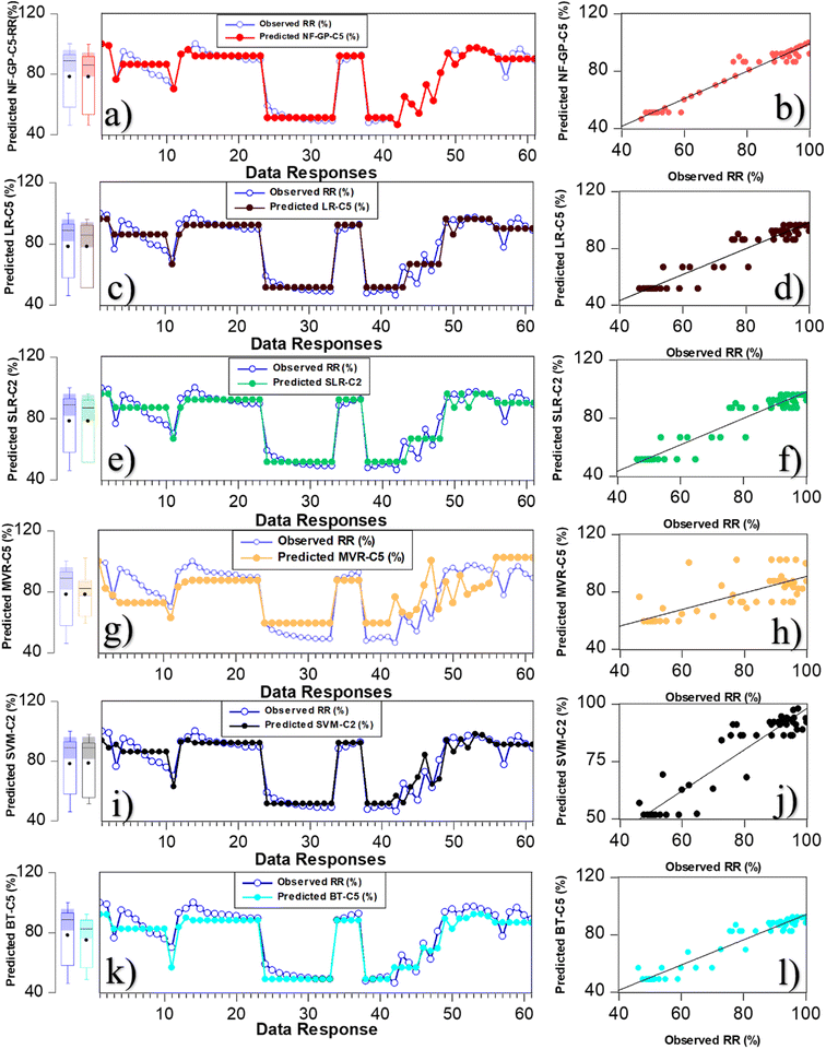 |
| | Fig. 7 Comparison of micropollutant rejection rate (%) data response alongside a scatter plot illustrating the performance of the superior predictive models NF-GP-5 (a and b), LR-C5 (c and d), SLR-C2 (e and f), MVR-C5 (g and h), SVM-C2 (i and j) and BT-C5 (k and l). | |
Table 4 Comparison of superior predictive performance of the NF-GP-5, LR-C5, SLR-C2, MVR-C5, SVM-C2 and BT-C5 models
| Models |
Verification phase |
| R2 |
R |
MSE |
RMSE |
MAE |
| NF-GP-C5 |
0.910 |
0.954 |
7.041 |
2.653 |
0.217 |
| LR-C5 |
0.762 |
0.873 |
18.637 |
4.317 |
0.005 |
| SLR-C2 |
0.739 |
0.860 |
20.471 |
4.525 |
0.198 |
| MVR-C5 |
0.563 |
0.750 |
104.227 |
10.209 |
0.993 |
| SVM-C2 |
0.726 |
0.852 |
21.521 |
4.639 |
0.281 |
| BT-C5 |
0.772 |
0.879 |
17.891 |
4.230 |
1.600 |
The predictive performance of the ML algorithm in estimating micropollutant removal efficiency was benchmarked against existing literature. Xu et al. explored the use of the Lindeman-Merenda-Gold (LMG) model to assess the impact of input variables, including the physiochemical characteristics of six distinct NF membranes and micropollutants, as experimental parameters on the rejection rate (%).44 The factor analysis associated with the LMG model revealed that membrane pore size and TMP have significant contribution in the micropollutant rejection. The predictive analysis conducted using the Random Forest Regression (RFR) model for optimizing the rejection prediction model yielded a R2 of 0.73, with the MAE and RMSE recorded at 6.92%, and 12.22% respectively. Zhu et al., compared the 10 ML algorithm including MLR, Bayesian regression (Bayes), SVM, ANN, extreme learning machine (ELM), and kNN and RF, GBDT, XGBoost and LightGBM for the effective prediction of micropollutant rejection rate (%) under forward osmosis (FO) operation.45 XGBoost-18 model, enhanced with SHAP, exhibited a coefficient of determination (R2) of 98% in predicting the micropollutant rejection rate (%), considering 18 significant factors related to the membrane, micropollutant, and experimental conditions. Mousavi and Sajjadi compared the ANN-quantitative structure–activity relationship (QSAR) model strategy for the prediction of 72 micropollutant removal rate in RO membranes.46 The ANN-QSAR model outperformed the MLR model, achieving higher accuracy with a R2 of 0.95 and a lower RMSE of 6.4224. Teychene et al., conducted research using a decision tree model to assess the performance of reverse osmosis (RO) and nanofiltration (NF) membranes in removing 22 different polar micropollutants, focusing on the removal rate (%).47 The decision tree analysis indicated that NF membrane separation is predominantly influenced by electrostatic interactions and size exclusion phenomena, while the RO membrane performance is chiefly determined by the diffusive transport of polar micropollutants. The present study into both supervised and unsupervised learning models, specifically NF-GP-C5, NF-SC-C5, SVM-C2, and BT-C5, demonstrated comparable predictive accuracies with minimal error margins, with NF-GP-C5 exhibiting the most superior predictive performance over all the combinations. This research indicated that employing feature engineering in conjunction with ML techniques shows promise for selecting optimal combinations of input variables, thereby achieving high prediction accuracy. Predicting micropollutant rejection efficiency may enable the design of membranes with optimal pore sizes, enhancing clean water production efficiency. Additionally, optimizing experimental conditions based on these predictions can reduce energy consumption and operational costs.
Conclusions
The ML algorithm including NF-GP, NF-SC, LR, SLR, MVR, SVM and BT ML were adeptly modeled and predicted the micropollutant removal efficiency, considering the influence of 14 input variables based on the influence of membrane characteristics, micropollutant properties, and filtration conditions. The feature engineering analysis revealed that a strategic combination of micropollutant property models holds significant potential in influencing and controlling the filtration performance of custom-designed functional membranes. MaxP, MinP, MW, and CS are dominant factors, attributed to their role in dictating the filtration mechanism of adsorption or sieving tendencies within the functional membrane. An inverse relationship was noted among crucial input variables, including Kow, MWCO, MCA, TMP, and C0. The constrained variability and scope of data points, in conjunction with intricate data distributions, can veil fundamental patterns, thus hindering the elucidation of definitive correlations. Among the combination, C5 showed demonstrated enhanced predictive capability for micropollutant removal rate efficiency under ML tools. Optimal prediction accuracy for rejection efficiency was attained using a NF-GP model, characterized by an optimal parameter setting with an R2 value of 0.965 and both RMSE and MAE values at 3.65. NF-GP and NF-SC showed superior predictive in rejection across all six combinations. SVM and BT excel over LR by adeptly managing non-linear data, offering greater flexibility, reducing overfitting, thriving in high-dimensional scenarios, and achieving better generalization. The modeling approach highlighted that adaptations in data combinations significantly influence the input variables, as revealed through feature engineering analysis. Feature engineering, combined with ML algorithms, exhibited exceptional capability in underlying intricate patterns within micropollutant properties, membrane attributes, and experimental conditions. This ML algorithm would prospect for employing sparse datasets to precisely predict the efficacy of membrane performance.
Data availability
Data for this article, including all descriptions of data types are available at https://pubs.acs.org/doi/10.1021/acs.est.1c04041.
Conflicts of interest
There are no conflicts to declare.
Acknowledgements
This publication is based upon work supported by King Fahd University of Petroleum & Minerals. The author(s) at KFUPM acknowledge the Interdisciplinary Research Center for Membranes & Water Security and DROC for the support received. This research was funded by the Deanship of Research Oversight and Coordination (DROC) at King Fahd University of Petroleum & Minerals (KFUPM) under the Interdisciplinary Research Center for Membranes and Water Security.
References
- Z. Wang, G. W. Walker, D. C. G. Muir and K. Nagatani-Yoshida, Environ. Sci. Technol., 2020, 54, 2575–2584 CrossRef CAS PubMed.
- M. Carere, A. Antoccia, A. Buschini, G. Frenzilli, F. Marcon, C. Andreoli, G. Gorbi, A. Suppa, S. Montalbano, V. Prota, F. De Battistis, P. Guidi, M. Bernardeschi, M. Palumbo, V. Scarcelli, M. Colasanti, V. D'Ezio, T. Persichini, M. Scalici, A. Sgura, F. Spani, I. Udroiu, M. Valenzuela, I. Lacchetti, K. di Domenico, W. Cristiano, V. Marra, A. M. Ingelido, N. Iacovella, E. De Felip, R. Massei and L. Mancini, J. Environ. Manage., 2021, 300, 113549 CrossRef CAS PubMed.
- M. Lim, D. Patureau, M. Heran, G. Lesage and J. Kim, Environ. Sci.: Water Res. Technol., 2020, 6, 1230–1243 RSC.
- Y. Luo, W. Guo, H. H. Ngo, L. D. Nghiem, F. I. Hai, J. Zhang, S. Liang and X. C. Wang, Sci. Total Environ., 2014, 473–474, 619–641 CrossRef CAS PubMed.
- M. Vecchiato, T. Bonato, C. Barbante, A. Gambaro and R. Piazza, Sci. Total Environ., 2021, 796, 149003 CrossRef CAS PubMed.
- J. F. Nure and T. T. I. Nkambule, J. Ind. Eng. Chem., 2023, 126, 92–114 CrossRef CAS.
- P. Bhatt, G. Bhandari and M. Bilal, J. Environ. Chem. Eng., 2022, 10, 107598 CrossRef CAS.
- E. Alonso, C. Sanchez-Huerta, Z. Ali, Y. Wang, L. Fortunato and I. Pinnau, J. Membr. Sci., 2024, 693, 122357 CrossRef CAS.
- Y. S. Khoo, P. S. Goh, W. J. Lau, A. F. Ismail, M. S. Abdullah, N. H. Mohd Ghazali, N. K. E. M. Yahaya, N. Hashim, A. R. Othman, A. Mohammed, N. D. A. Kerisnan, M. A. Mohamed Yusoff, N. H. Fazlin Hashim, J. Karim and N. salmi Abdullah, Chemosphere, 2022, 305, 135151 CrossRef CAS PubMed.
- M. Heiranian, H. Fan, L. Wang, X. Lu and M. Elimelech, Chem. Soc. Rev., 2023, 52, 8455–8480 RSC.
- A. Matin, S. M. S. Jillani, U. Baig, I. Ihsanullah and K. Alhooshani, J. Environ. Manage., 2023, 338, 117682 CrossRef CAS PubMed.
- M. An, L. Gutierrez, A. D'Haese, L. Tan, A. Verliefde and E. Cornelissen, Desalination, 2023, 565, 116861 CrossRef CAS.
- D. Lu, X. Ma, J. Lu, Y. Qian, Y. Geng, J. Wang, Z. Yao, L. Liang, Z. Sun, S. Liang and L. Zhang, Desalination, 2023, 564, 116748 CrossRef CAS.
- A. Mohammed, H. Alshraideh and F. Alsuwaidi, Desalination, 2024, 574, 117253 CrossRef CAS.
- H. M. Chang, Y. Xu, S. S. Chen and Z. He, Sci. Total Environ., 2022, 838, 156009 CrossRef CAS PubMed.
- Z. Haider Jaffari, H. Jeong, J. Shin, J. Kwak, C. Son, Y. G. Lee, S. Kim, K. Chon and K. Hwa Cho, Chem. Eng. J., 2023, 466, 143073 CrossRef CAS.
- N. D. Viet and A. Jang, J. Cleaner Prod., 2023, 389, 136023 CrossRef CAS.
- P. Dansawad, Y. Li, Y. Li, J. Zhang, S. You, W. Li and S. Yi, Adv. Membr., 2023, 3, 100072 CrossRef.
- G. Ignacz, N. Alqadhi and G. Szekely, Adv. Membr., 2023, 3, 100061 CrossRef.
- J. W. Barnett, C. R. Bilchak, Y. Wang, B. C. Benicewicz, L. A. Murdock, T. Bereau and S. K. Kumar, Sci. Adv., 2020, 6, eaaz4301 CrossRef CAS PubMed.
- P. Priya, T. C. Nguyen, A. Saxena and N. R. Aluru, ACS Nano, 2022, 16, 1929–1939 CrossRef CAS PubMed.
- N. Baig, S. I. Abba, J. Usman, M. Benaafi and I. H. Aljundi, Environ. Sci.: Adv., 2023, 2, 1446–1459 CAS.
- N. K. Khanzada, M. U. Farid, J. A. Kharraz, J. Choi, C. Y. Tang, L. D. Nghiem, A. Jang and A. K. An, J. Membr. Sci., 2020, 598, 117672 CrossRef CAS.
- N. Jeong, T. H. Chung and T. Tong, Environ. Sci. Technol., 2021, 55, 11348–11359 CrossRef CAS PubMed.
- T. Zhu, Y. Zhang, C. Tao, W. Chen and H. Cheng, Sci. Total Environ., 2023, 857, 159348 CrossRef CAS PubMed.
- H. Wang, J. Zeng, R. Dai and Z. Wang, Environ. Sci. Technol., 2024, 58, 5878–5888 CrossRef CAS PubMed.
- Y. Wu, M. Chen, H. J. Lee, M. A. Ganzoury, N. Zhang and C. F. De Lannoy, ACS ES&T Eng., 2022, 2, 1574–1598 Search PubMed.
- Y. Liu, K. Wang, Z. Zhou, X. Wei, S. Xia, X. M. Wang, Y. F. Xie and X. Huang, Environ. Sci. Technol., 2022, 56, 15220–15237 CrossRef CAS PubMed.
- F. Wang, W. Wang, H. Wang, Z. Zhao, T. Zhou, C. Jiang, J. Li, X. Zhang, T. Liang and W. Dong, Sci. Total Environ., 2023, 883, 163610 CrossRef CAS PubMed.
- P. Masuodi, F. Bahmanzadegan, A. Hemmati and A. Ghaemi, Case Stud. Chem. Environ. Eng., 2024, 9, 100750 CrossRef CAS.
- S. P. Sun, T. A. Hatton, S. Y. Chan and T. S. Chung, J. Membr. Sci., 2012, 401–402, 152–162 CrossRef CAS.
- T. Puspasari, N. Pradeep and K. V. Peinemann, J. Membr. Sci., 2015, 491, 132–137 CrossRef CAS.
- J. Wang, L. Wang, C. Xu, R. Zhi, R. Miao, T. Liang, X. Yue, Y. Lv and T. Liu, Chem. Eng. J., 2018, 332, 787–797 CrossRef CAS.
- Y. ying Zhao, X. mao Wang, H. wei Yang and Y. F. Xie, J. Membr. Sci., 2018, 563, 734–742 CrossRef.
- B. He, H. Peng, Y. Chen and Q. Zhao, J. Membr. Sci., 2020, 608, 118202 CrossRef CAS.
- X. D. Weng, Y. L. Ji, R. Ma, F. Y. Zhao, Q. F. An and C. J. Gao, J. Membr. Sci., 2016, 510, 122–130 CrossRef CAS.
- A. F. Schmidt and C. Finan, J. Clin. Epidemiol., 2018, 98, 146–151 CrossRef PubMed.
- L. Davies, arXiv, 2016, preprint, arxiv:1605.04542, DOI:10.48550/arXiv.1605.04542.
- A. T. C. Goh and W. G. Zhang, Eng. Geol., 2014, 170, 1–10 CrossRef.
- U. Alhaji, E. Chinemezu and S. Isah, Bioresour. Technol. Rep., 2022, 19, 101167 CrossRef.
- J. Xing, K. Luo, H. Wang, Z. Gao and J. Fan, Energy, 2019, 188, 116077 CrossRef.
- G. Wang, J. K. S. Paw, J. Pasupuleti, C. T. Yaw, T. Yusaf, A. N. Abdalla and Y. Cai, Case Stud. Therm. Eng., 2024, 53, 103729 CrossRef.
- J. R. Jang, IEEE Trans. Syst. Man Cybern., 1993, 23, 665–685 CrossRef.
- R. Xu, Z. Zhang, C. Deng, C. Nie, L. Wang, W. Shi, T. Lyu and Q. Yang, Environ. Res., 2024, 244, 117935 CrossRef CAS PubMed.
- T. Zhu, Y. Zhang, Y. Li, C. Tao, Z. Cao and H. Cheng, J. Environ. Chem. Eng., 2023, 11, 110847 CrossRef CAS.
- S. L. Mousavi and S. M. Sajjadi, RSC Adv., 2023, 13, 23754–23771 RSC.
- B. Teychene, F. Chi, J. Chokki, G. Darracq, J. Baron, M. Joyeux and H. Gallard, Water Supply, 2020, 20, 975–983 CrossRef CAS.
|
| This journal is © The Royal Society of Chemistry 2024 |
Click here to see how this site uses Cookies. View our privacy policy here. 
 Open Access Article
 This Open Access Article is licensed under a Creative Commons Attribution-Non Commercial 3.0 Unported Licence
 a,
Sani I. Abba
a,
Sani I. Abba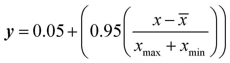
 ) and the kernel function (K(x,xi)) for constrained optimization problems are expressed as follows: