
 Open Access Article
 This Open Access Article is licensed under a
 Creative Commons Attribution 3.0 Unported Licence
Unsupervised learning and pattern recognition in alloy design
Ninad
Bhat
a,
Nick
Birbilis
b and
Amanda S.
Barnard
 *c
*c
aSchool of Engineering, Australian National University, Acton, Australia
bFaculty of Science, Engineering and Built Environment, Deakin University, Waurn Ponds, Australia
cSchool of Computing, Australian National University, Acton, Australia. E-mail: amanda.s.barnard@anu.edu.au
First published on 28th October 2024
Abstract
Machine learning has the potential to revolutionise alloy design by uncovering useful patterns in complex datasets and supplementing human expertise and experience. This review examines the role of unsupervised learning methods, including clustering, dimensionality reduction, and manifold learning, in the context of alloy design. While the use of unsupervised learning in alloy design is still in its early stages, these techniques offer new ways to analyse high-dimensional alloy data, uncovering structures and relationships that are difficult to detect with traditional methods. Using unsupervised learning, researchers can identify specific groups within alloy data sets that are not simple partitions based on metal compositions, and can help optimise and develop new alloys with customised properties. Incorporating these data-driven methods into alloy design speeds up the discovery process and reveals new connections that were not previously understood, significantly contributing to innovation in materials science. This review outlines the key scientific progress and future possibilities for using unsupervised machine learning in alloy design.
 Ninad Bhat | Mr Ninad Bhat is a PhD candidate at the School of Engineering, Australian National University. His research focuses on developing machine learning models for designing aluminium alloys with optimised properties. Before pursuing his PhD, Ninad completed his Bachelor's and Master's degrees from the Indian Institute of Technology Bombay, where he majored in Metallurgical Engineering and Materials Science. |
 Nick Birbilis | Professor Nick Birbilis is the Executive Dean of the Faculty of Science, Engineering and Built Environment at Deakin University, Australia. His research has sought to rationalise the behaviour of engineering alloys from a deterministic perspective. He has interests including computational studies of materials and machine learning tools to accelerate materials discovery. His awards include the H. H. Uhlig Award, the Australian Academy of Technological Sciences and Engineering Batterham Medal, along with recognition as a Fellow of ASM International, The Electrochemical Society, International Society of Electrochemistry, NACE (National Association of Corrosion Engineers) and Engineers Australia. |
 Amanda S. Barnard | Professor Amanda Barnard is the Deputy Director of the School of Computing at the Australian National University, and leader of Computational Science. Her research occupies the intersection of high-performance computing, machine learning, materials science and nanotechnology, focussing on method development addressing small data challenges, (causal) structure–property relationships and explainable AI. She is a Fellow of the Australian Institute of Physics, the Australian Computer Society and the Royal Society of Chemistry. Her awards include the Physical Scientist of the Year from the Prime Minister of Australia, the Frederick White Prize from the Australian Academy of Science, the ACS Nano Lectureship from the American Chemical Society, and the Feynman Prize (Theory) from the Foresight Institute. In 2022 she was appointed a Member of the Order of Australia for services to computational science. |
1 Introduction
Materials design has undergone a significant change in recent years, seeing increased adoption of machine learning (ML)1 to overcome limitations of empirical methods, which have been principally based on domain expertise and trial-and-error experimentation.2–4 This has been supported by the availability of large-scale materials data, computational resources and collaboration between the materials, statistics and computer science communities.5 Machine learning offers a new paradigm for materials design,6–10 uncovering relationships, patterns and trends that are otherwise obscured in conventional research. By leveraging computational and experimental results, ML models can predict material properties,11–14 optimise processing routes,15,16 and recommend superior material compositions.17 The integration of ML into materials development not only accelerates the discovery process18 but enables exploration of material spaces that were previously deemed too complex or computationally expensive to investigate.19–23One of the key strengths of ML is its versatility. A single ML method can be used for multiple tasks, and applied to multiple data sets with entirely different volume, veracity and distributions. Supervised learning techniques are ideal for predictive tasks where historical data can be learned to predict future outcomes.24,25 These models learn from labelled data sets, where input features are mapped to known outputs, allowing for the prediction of material properties based on compositional and processing variables. This predictive capability is invaluable in the design of alloys,26 polymers,27 and nanomaterials.28–30 By systematically exploring the relationship between input variables and material properties, supervised ML models can guide the design of new materials with optimised characteristics.31–34 Alternatively, unsupervised learning identifies hidden patterns within data, regardless of the target properties,35 and can inform new research direction and investments, well in advance of applications. While unsupervised learning is used throughout materials informatics, currently this is an underdeveloped area of metal alloy design, with excellent potential to extract latent knowledge buried in high dimensional combinatorial data. Examples are limited, but include nanoalloys,36–40 high entropy alloys,41–58 and industrial Al and Mg alloys discussed in more detail in the coming sections.
1.1 Alloys and applications
Alloys play a crucial role in a wide range of industries, making them essential in most aspects of our modern lives, including communications, healthcare, transport, infrastructure and our supply of water and electricity. For example, in aerospace,59 high-strength, lightweight alloys such as aluminium and titanium are essential for constructing aircraft components, where balancing strength and weight is critical.60 In the automotive industry,61,62 aluminium alloys are extensively used to reduce vehicle weight and improve fuel efficiency.62 In construction,63 steel alloys are utilised due to their durability and load-bearing capacity.64 In electronics, copper alloys are widely used in electrical wiring and connectors, due to their excellent conductivity and corrosion resistance.65Alloys are materials composed of two or more metallic elements, often combined with non-metallic elements, to enhance their properties compared to their individual components.66 The primary objective of creating alloys is to achieve superior strength, hardness, fatigue or fracture resistance, corrosion resistance, or other desired characteristics tailored to specific applications.67 Each alloy is typically defined by the primary component, known as the 'base metal'. In the case of steel, one of the most widely used alloys, the primary components are iron and carbon.68 The addition of carbon to iron significantly increases the material's strength and hardness, making steel viable for modern construction and manufacturing.68
Alloys are further categorised based on their main alloying elements, using a range of internationally recognised numbering systems that reflect industry standards.69,70 For example, wrought aluminium alloys are divided into eight series (denoted by Nxxx), such as 6xxx (aluminium–magnesium–silicon) and 7xxx (aluminium–zinc) alloys, based on the primary alloying element.71 Similarly, magnesium alloys are organised into series such as AZ, where aluminium and zinc are the key alloying elements, and AM, where aluminium and manganese are predominant.71 More information on this numbering system and the alloy designations can be found in ref. 72.
Broadly, there are two main types of alloy: substitutional alloys,73 where atoms of the alloying element replace atoms of the base metal, and interstitial alloys,74 where smaller atoms fit into the spaces between the base metal atoms (an exception being a small number of amorphous alloys, that are non-crystalline). Alloys are produced by blending the base metal with the alloying elements. The most common method to achieve this is via melting.75 A molten alloy mixture is then cooled or cast into a solidified structure. Other methods include powder metallurgy,76 where metals are blended in powdered form and then fused together, and chemical vapour deposition,77 used for creating thin-film alloys. The production of alloys requires precise control over the composition, temperature, and cooling rate to achieve the desired microstructure.78 The resulting microstructure of the alloy determines its mechanical and physical properties. This complexity is a significant challenge in alloy design, as even minor variations can lead to substantial differences in performance.
After solidification, further processing is often required to modify the microstructure and enhance the properties of the alloy. Post-solidification processing, termed thermo-mechanical processing, can also be highly complex. These processes include rolling,79 forging,80 heat-treatment,71 and solid–state processes that also include controlled quenching81 (for example, to form martensite in steels) or precipitation hardening82 (the basis for achieving aerospace aluminium alloys, necessary for aviation).
For these reasons designing alloys is inherently complicated, occupying a vast high dimensional combinatorial design space71,83,84 where the number of potential multi-component alloys is difficult to explore experimentally. The process of optimising alloys often involves property trade-offs, since enhancing one characteristic, such as strength, can negatively impact another, such as ductility.85 The growing demand for sustainable materials further complicates alloy design, as it adds the pressure of developing alloys that not only fulfil technical requirements but also minimise environmental impact and cost.86 To achieve these objectives, traditional alloy design has followed a trial-and-error approach, where the selection of elements and their proportions is guided by the experience and intuition of materials scientists.82,87 This often involves systematically varying a small subset of alloying element concentrations or processing conditions to achieve the desired properties,88–90 or rationalising the underlying mechanisms through complex and time-consuming characterisation methods.
2 Research questions
As the demand for new materials with specific properties increases,86,91 there is a growing need for more efficient and predictive design approaches, that can narrow down the possibilities before attempting to train structure–property models. Conventional methods of alloy development,92,93 are time-consuming and resource-intensive,94 and so researchers are increasingly turning to data-driven techniques to address some of the challenges related to traditional materials design processes.95,96Unsupervised learning techniques have emerged as powerful tools in this context, offering the ability to analyse complex, high-dimensional data sets that are common in materials science,97,98 without the added cost of measuring properties. The objective of unsupervised learning is to identify patterns in an unlabelled data set when no information on the physicochemical properties is available. Common unsupervised learning tasks include cluster analysis99 and dimensionality reduction (DR).100 Cluster analysis involves the grouping of data instances (individual structures) based on their similarities or differences in a high dimensional space using distance metrics. Representative structures (prototypes) can be identified from each cluster centroid. DR involves obtaining lower-dimensional representations of data, which allows simplification and acceleration of model training and improvement in model generalisability. DR includes methods that reduces the number of features needed to describe an alloy, and methods that reduce the number of alloys to the most influential and important subset.101 These methods enable researchers to uncover hidden patterns, reduce the complexity of data, and identify novel outliers that may correspond to new, previously unexplored materials or properties. Applications of these methods to alloy design are still relatively rare, so there is a considerable untapped opportunity to address important research questions in the field.
2.1 The curse of dimensionality
One of the key challenges in alloy design is the high dimensionality102 and low volume of data. This results in “curse of dimensionality”103–105 and makes it difficult to analyse using traditional methods. Dimensionality reduction techniques can address this issue,84 by reducing the number of independent variables (features), while retaining the essential information. These methods simplify the analysis and help in identifying the underlying patterns in the data set.1062.2 Recognising hidden patterns
The detection of patterns in high-dimensional data is another critical use of unsupervised learning in alloy design.107 Alloys exhibit complex relationships between composition, processing, and properties, which are often non-linear.108 Unsupervised learning algorithms, such as clustering and manifold learning, are particularly well-suited for uncovering these patterns without labelling data. Clustering techniques can also group similar data instances based on their features, which can help to focus research.2.3 Identifying special cases
In virtually every data set, there are special cases that can be useful or detrimental to the training of models and, ultimately, to predictions.109–111 Examples include archetypes, prototypes, stereotypes, and outliers. Archetypes are the ‘pure’ instances (on the convex hull), prototypes are the representative instances (or average in high-dimensional space), stereotypes are instances with intrinsic importance (such as thermodynamically stable structures), and outliers are anomalies that can be due to poor sampling, errors in data collection, or rare events. Anomalies can also be caused by defects in the alloys, including microstructural imperfections or processing artefacts.112 Identifying these defect-related outliers is important for ensuring the quality and reliability of the final alloy produced.1132.4 Structure of the review
This tutorial review has been structured around the unsupervised learning methods used to address these research questions, with sections describing different approaches to dimensionality reduction (Section 3), manifold learning (Section 4), clustering (Section 5), outlier detection (Section 6) and semi-supervised learning (Section 7). These sections contain brief summaries of different methods, highlighting their advantages and disadvantages, and recommended uses in alloy design. Each section concludes with a survey of some previous applications to alloys and alloying metals, to demonstrate the utility and highlight how new knowledge can be gained. To date there are few instances of unsupervised learning of metal alloys and but these applications are aggregated in Table 1, cross referenced by metals, ML methods and applications. As this area of research is still at an early stage, this review provides a foundation for future studies and complements other reviews covering supervised learning of structure–property relationships.114–118| Author | Year | Application(s) | Base metal(s) | ML method(s) | Reference |
|---|---|---|---|---|---|
| Sun et al. | 2017 | Biomedical | Nano Ag | k-Means | 119 |
| Syuhada et al. | 2018 | Chemical analysis | Al, Ti, Cu, Zn | PCA | 120 |
| Sun et al. | 2018 | Biomedical | Nano Ag | SOM | 121 |
| Shirinyan et al. | 2019 | Magnetic applications (sensors, electromagnets) | Fe | SOM | 122 |
| Verma et al. | 2019 | Structural | Fe | t-SNE | 123 |
| Jha et al. | 2019 | Aerospace | Ti, Al, Cr, V | SOM | 124 |
| Krishnamurthy et al. | 2019 | Structural | Fe | t-SNE | 125 |
| Verma et al. | 2019 | Structural | Fe | t-SNE | 126 |
| Sun et al. | 2019 | Biomedical | Nano Ag, Pt | t-SNE, SOM | 127 |
| Parker et al. | 2020 | Electrocatalysis | Nano Pt | ILS | 128 |
| Dasgupta et al. | 2020 | Catalytic design | Single atom alloy | LOFA | 129 |
| Tian et al. | 2020 | Structural | Cu, Zr | RANSAC | 130 |
| Parker et al. | 2020 | Electrocatalysis | Nano Pt | AA | 131 |
| Esterhuizen et al. | 2021 | Catalysis | Rh, Pd, Pt, Ir | PCA | 132 |
| Jung et al. | 2021 | Structural | Fe | AE | 133 |
| Liu et al. | 2021 | Thermal coating | Al | UMAP | 134 |
| Esterhuizen et al. | 2021 | Catalysis | Ir, Pt, Pd, Rh | PCA | 135 |
| Subbarao et al. | 2021 | Aerospace, biomedical | Ti, Al, V | PCA | 136 |
| Kim et al. | 2021 | Structural | Fe | AE | 137 |
| Yin et al. | 2021 | Structural, automobile | HEA | AE | 138 |
| Lee et al. | 2022 | Structural, automobile | HEA | k-Means | 139 |
| Chintakindi et al. | 2022 | Marine | Ni | PCA | 140 |
| Lee et al. | 2022 | Structural, Automobile | HEA | k-Means | 141 |
| Xin et al. | 2022 | Structural | Si | PCA | 142 |
| Wenzlick et al. | 2022 | Structural | Fe | LOFA | 113 |
| Bundela et al. | 2022 | Structural, automobile | HEA | PCA | 143 |
| Foggiatto et al. | 2023 | Sensors | Fe, Ga | PCA | 144 |
| Ahmad et al. | 2023 | Microstructure modelling | Binary Alloy | AE | 145 |
| Bhat et al. | 2023 | Aerospace | Al | ILS | 146 |
| Ghorbani et al. | 2023 | Automobile, electronics | Mg | t-SNE | 147 |
| Chen et al. | 2023 | Biomedical | Al, Ni | UMAP | 148 |
| Tiwari et al. | 2023 | Structural | Al | k-Means | 149 |
| Ting et al. | 2023 | Electrocatalysis | Nano Ru | ILS | 150 |
| Roncaglia et al. | 2023 | Catalysis, biomedical | Ag, Au, Pd, Cu | PCA, k-means | 151 |
| Vela et al. | 2023 | Aerospace | W, Mo, V, Ta, Nb, Al | UMAP | 152 |
| Fetni et al. | 2023 | Microstructure modelling | Binary Alloy | AE | 153 |
| Moses et al. | 2024 | Automobile, electronics | Mg | k-Means | 154 |
| Lie et al. | 2024 | Structural | Fe | t-SNE | 155 |
| Usuga et al. | 2024 | Catalysis | Bimetallic alloys | UMAP | 156 |
3 Dimensionality reduction
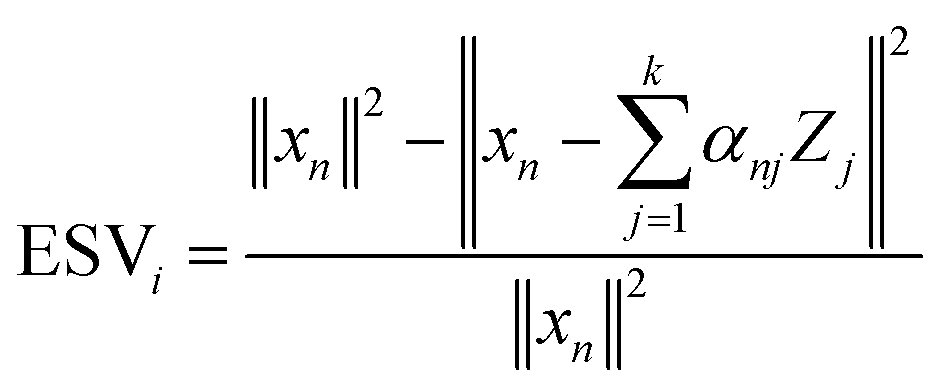
As mentioned above, depending on the number of structural features and chemical features, alloy data sets can be high-dimensional. High-dimensional data is not intuitive for visualisation and produces complicated models that are slow to optimise, train and use in practice. Many different unsupervised algorithms are available to reduce the feature space and improve the efficiency of ML models, the aim of which is to minimise the information loss and maximise the impact of the information retained. Dimensionality reduction methods are applied before ML models are trained, and the most convenient way to evaluate a dimension reduction method is statistically by calculating the Explained Sample Variance (ESV).The ESV is a quality measure of the deviation between the nth original data instance xn and the derived data instance  and is given by:
 | (1) |
By evaluating these ESV values, it is possible to state which alloys will be well described by a model. The ESV ranges between 0 and 1, where 1 is a perfect match. No conclusions should be made for alloys where the ESV is low because these sample instances will be poorly described by a model.
3.1 Feature selection
Feature selection is a crucial preliminary step for reducing the dimensionality of a data set while preserving its most important features.157,158 The goal is to capture essential information with minimal redundancy, thereby improving the performance and interpretability of models.159Feature selection can be approached through data-driven, domain-driven, and model-driven methods, each with its own focus and advantages. Data-driven feature selection relies on the statistical properties of the data set to eliminate irrelevant or redundant features. For example, when features are highly correlated they provide similar information, so removing one of the correlated features can reduce redundancy without losing valuable information.160 Similarly, features with low variance across the data set typically contribute little to distinguishing between data instances and can be excluded to simplify the model and reduce noise.161
Domain-driven feature selection leverages expert knowledge in alloy design to determine which features are less important or irrelevant. For instance, in alloy data sets, domain experts can choose to remove an element due to its toxicity,162 thereby focusing the analysis on more significant features. Finally, model-driven feature selection uses insights gained from preliminary modelling to identify the most important features.161 This approach often involves training a model and assessing which features contribute most significantly to its predictions. For example, certain machine learning models, such as decision trees or random forests, generate feature importance scores163 that indicate the relevance of each feature to the model architecture. Features with low importance can then be removed, streamlining the model without compromising its performance.
When these methods fail to address the problem, or are inappropriate, transforming the data using feature engineering can help. A survey of feature selection across materials science can be found in ref. 164, and additional examples in ref. 165 and 166.
3.2 Principal component analysis
Principal components analysis (PCA) converts a set of potentially correlated features into a set of linearly uncorrelated variables; the principal components (PCs).167 PCA takes an n × m data matrix, X (of n materials and m structural features) and uses an orthogonal linear matrix transformation to express the original data as a linear combination of scores and loadings, described by: | (2) |
One of the primary advantages of PCA is its simplicity and computational efficiency, making it ideal for quickly analysing large data sets. Additionally, PCA is deterministic, ensuring consistent results without the variability that can affect other methods described in upcoming Sections of this review. However, PCA is limited to linear transformations and may not effectively capture complex, non-linear relationships in the data (which is often the case with alloy data sets168). Additionally, PCA can be heavily influenced by outliers, and in alloy data sets where outliers might indicate unusual material behaviour or errors, this sensitivity can distort results unless managed carefully. Such effects can be minimised by using robust PCA and outlier detection methods in combination.169 This method has been used widely in materials science for many years.170 Outlier detection will be discussed in Section 6.
3.3 Singular value decomposition
Singular Value Decomposition (SVD) is another technique used to reduce the dimensionality of the data while preserving its most important features.171 SVD does this by projecting the original data into a lower-dimensional space that captures the most significant variations. Given a data set represented by a matrix A of dimensions m × n, where m is the number of data instances (e.g. number of alloys) and n is the number of features (e.g. alloy composition), the SVD of A is defined as:| A = UΣVT | (3) |
The reduced representation Ak of the original matrix A is given by:
| Ak = UkΣkVkT | (4) |
SVD is effective at separating signal from noise in data, making it particularly valuable for alloy data sets that may contain measurement errors.172 By focusing on the largest singular values and their corresponding vectors, SVD can significantly reduce the impact of noise, and can be can be adapted to handle missing data,173 which is especially beneficial for alloy data sets with incomplete measurements. However, like PCA, SVD is sensitive to outliers and does not capture the non-linear interactions that are crucial in understanding alloy behaviour. SVD has been useful in the processing of images in materials science.174,175
3.4 Archetypal analysis
Archetypal analysis (AA),176 also known as principal convex hull analysis, is a matrix factorisation method that aims to approximate all alloy instances in a data set as a linear combination of extremal points. A given data set of n alloys described by m features is represented by an n × m matrix, X. Archetypal analysis seeks to find a k × m matrix Z such that each data instance can be represented as a mixture of the k archetypes. This is achieved by minimizing the residual sum of squares, under some constraints: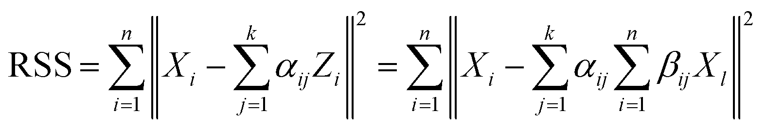 | (5) |
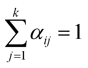 with αij ≥ 0 and i = 1, …, n. and
 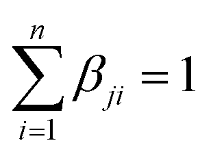 with βji ≥ 0 and j = 1, …, k. The first constraint requires the data to be approximated by convex combinations of the archetypes, whilst the second constraint requires that the archetypes are convex combinations of the data. The resultant archetypes form a convex hull of the data set, but they need not be present in the original set to be identified.
Archetypal analysis provides a set of archetypes that represent the pure types within the data set. Using archetypes of describe a set can make the results more interpretable,177 since each measured or hypothetical instance is described as a mixture of systems that are easy to understand. However, it is important when using AA that the data is cleaned appropriately, as it uses a least-squares optimisation, which is heavily influenced by the presence of outliers. This approach has been used in nanoinformatics29 to identify archetypal nanoparticle morphologies.97,101,178,179
3.5 Kohonen maps
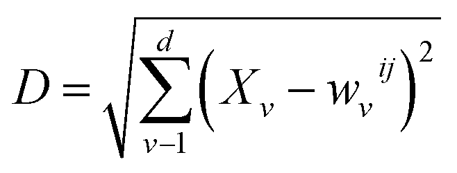
A Kohonen network,180 or self-organisation map (SOM), is an unsupervised artificial neural network181 for non-linearly mapping high-dimensional spaces into low-dimensional spaces, with the advantage of retaining the intrinsic topological relationship of the input data set. SOMs are ideal for visualising multi-dimensional data sets in a single two-dimensional image,182 and have been recently used to create surface texture maps of metallic nanoparticles suitable for use as material fingerprints.183The basic units of a SOM are neurons which are best organised on hexagonal grids. All neurons can be arranged in a planar (approximate) rectangle, with periodic boundary conditions to connect the upper and lower boundaries and the right and left boundaries so that the SOM plane occupies the surface of a torus. The weights of all neurons are initialised using random numbers. During each training step every neuron competes against all others until each original data instance finds the one neuron that is closest to it in Euclidean space, referred to as the best matching unit (BMU). Given an input data instance x, and the weight of neuron i, j is wij, then the Euclidean distance D is:
 | (6) |
 | (7) |
 | (8) |
 | (9) |
One of the key benefits of SOMs is their ability to preserve the topological structure of the data, meaning that alloys with similar properties or compositions will be mapped close to each other on the grid. This topological preservation is particularly valuable when trying to understand relationships and patterns in complex alloy data sets; separating groups that are dissimilar, and the separation distance representing just how dissimilar they are. However, an important consideration in SOM training is the number of epochs, which is a important hyper-parameter. A large number of epochs will result in over-training, leading to a waste of computational resources, but a small number of epochs will result in under-training, and dissimilar alloys may be adjacent in the final SOM, reducing the resolution. It is possible to measure the number of void neurons that have no weight and stop the training when this number stops decreasing over a threshold after, for instance, nepoch = 5, to improve efficiency and autonomy.184 This has been useful in processing spectroscopic data in materials science.185–187
3.6 Autoencoders
Autoencoders are a class of neural networks used primarily for unsupervised learning.188 Their main objective is to learn a compressed representation (encoding) of input data, which can then be used for tasks such as dimensionality reduction,189 feature extraction,190 and anomaly detection.191An autoencoder consists of two main components: an encoder E(·) and a decoder D(·). The encoder compresses the input data x into a lower-dimensional representation z, often referred to as the latent space or code. The decoder then attempts to reconstruct the original input from this compressed representation. The overall structure can be summarised as follows:
| Encoder: z = E(x) = f(Wex + be) | (10) |
Decoder: ![[x with combining circumflex]](https://www.rsc.org/images/entities/i_char_0078_0302.gif) = D(z) = g(Wdz + bd) = D(z) = g(Wdz + bd) | (11) |
| Reconstruction: = D(E(x)) | (12) |
The goal of training an autoencoder is to minimise the difference between the input x and the reconstructed output . This difference is quantified by a loss function, typically the mean squared error (MSE):
 | (13) |
Autoencoders work better in dimensionality reduction in data set non-linear relationships when compared to methods such as PCA.192 Their flexible architecture allows for task-specific customisation, and they operate without needing labelled data, making them ideal for unsupervised learning scenarios. However, they also come with challenges, such as the need for careful hyper-parameter tuning, potential difficulties in capturing complex data distributions, and a risk of over-fitting, particularly with small data sets.193 These factors can limit their effectiveness and generalisability in some applications, but they have successfully been applied to materials science problems.194,195
3.7 Reducing alloy data
In alloy research, PCA has primarily been used to reduce the feature spaces in prreparation for either clustering120,196 or training regression models to predict properties.142 For example, PCA was used to cluster alloy samples using Laser-Induced Breakdown Spectroscopy (LIBS) data.120 Copper and aluminium presented distinct clusters in the PC plot, as shown in Fig. 1. Brass showed a wide spread in the plot, which could be attributed to the presence of both copper and zinc in high concentrations. However, using LIBS with PCA proved to be a viable method to identify elements in alloys. | ||
| Fig. 1 Principal component plot for Al, Cu, and Brass alloys, demonstrating clear separation between the alloy groups. Reproduced from ref. 197, with permission from Institute of Physics Publishing, Creative Commons Attribution 3.0 licence. | ||
PCA has also been used to reduce the dimensionality of features in molten steel for the prediction of alloying element yield.142 Using PCA, the features set was reduced such that the cumulative contribution rate of PCs extracted is above 90%, which lead to reduction of dimensions form 16 to 11. These principal components were used as features to train a deep neural network (DNN) to predict alloying yield. The PCA-DNN model demonstrated better performance compared to DNN models trained on the entire feature set, achieving a 0.03 increase in the R2 score for predicting silicon yield.
Self-organising maps have been used in design of high-temperature Ti alloys and magnetic alloys.107,124 By using alloy concentrations as input features, SOMs grouped AlNiCo alloys into 64 distinct units.107 SOM showed a strong correlation between ((BH)max and (BH)max/mass, as shown in Fig. 2. Additionally, studying the variation of magnetic energy density in the maps, it was observed that the top 10 alloys were concentrated in three adjacent units. This proximity suggests a meaningful correlation in the underlying structure of these alloys. SOMs were also used to group Ti alloys, using compositions of equilibrium α-Ti (hexagonal close-packed Ti) and β-Ti (body-centered-cubic Ti) phases calculated through CALPHAD as features.124
 | ||
| Fig. 2 SOM map showing strong correlations between ((BH)max and (BH)max/mass, and Br and Mr. Reproduced from ref. 107, with permission from Taylor & Francis, Copyright (2017). | ||
Archetypal analysis (AA) has been employed in metallic systems to identify seven distinct archetypes in platinum nanoparticles, which were subsequently mapped to seven different nanoparticle within the data set, as illustrated in Fig. 3. Although the application of AA in alloy research remains under-explored, it has been successfully use in materials research to identify unique and special compositions198 and structures,178,179,199 providing insights into the underlying patterns within complex data sets. This is a potential area of development for alloys, to reduce the larger sets of hypothetical alloys to the archetypes that may be reflective of particularly application domains.
 | ||
| Fig. 3 Example of archetypal analysis of platinum nanoparticle, showing (a) the data distributed with respect to the seven archetypes on a simplex plot (the size of points reflect the relative size of the particles), and (b) the seven nanoparticles in the data set closest matched archetypes. Reproduced from Reference with permission from Institute of Physics Publishing (IOPP), Copyright (2020). | ||
Autoencoders have been used for feature extraction and dimensionality reduction in the study of alloys.133,137,138,145,153,200 These models are primarily employed to reduce the dimensionality of microstructural images, transforming high-dimensional data into a lower-dimensional latent space representation. This latent space facilitates the identification of key features essential for understanding the properties of alloys200 and are also used for training additional machine learning models aimed at optimising microstructures.133,145,153 The reduced latent space in phase field modelling data was utilised to train an Long Short-Term Memory (LSTM) neural network model for predicting microstructure evolution, resulting in a validation loss of 0.0082.153
4 Manifold learning
An alternative way to simultaneously reduce the dimensionality of a high-dimensional alloy data set and visualise the distribution is to use manifold learning. Manifold learning is a non-linear unsupervised approach that generalizes the linear framework of PCA and projects high-dimensional data onto a low-dimensional space.201 Methods include multi-dimensional scaling202 (MDS), locally linear embedding203 (LLE), isometric mapping204 (isomap), spectral embedding205 (SE) and uniform manifold approximation and projection206 (UMAP). Each have different properties and advantages: SE or MDS ensures data instances near to each other are still close in the low dimensional space; LLE maintains the distance within the local neighbourhood; isomap preserves the geodesic distances between all data; and UMAP can result in better visualisation and significantly faster training than the alternatives. Manifold learning can offer a powerful way of visualising relationships.4.1 t-Distributed stochastic neighbor embedding
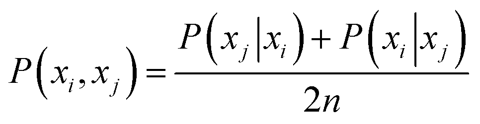
t-SNE has been widely used in materials science due to the inherent tunability that can aid in visualisation.207 t-SNE groups data instances based on local clustered structure by converting affinities into Gaussian joint probabilities. For n objects xi in d dimension the t-SNE uses the conditional probability that xj would be picked as a neighbour given xi is expressed as: | (14) |
 | (15) |
For the low-dimensional counterparts, yi of the high-dimensional data xi, a Student t-distribution with a degree of freedom one is used to compute the joint probabilities Q(yi, yj) as:
 | (16) |
This distribution is heavy-tailed so that dissimilar objects in low-dimensional space can be modelled even if they are far apart. The optimisation objective is to equate P(xi, xj) and Q(xi, xj), which means minimising the cost function  .
.
By tuning the t-SNE hyper-parameters to achieve a clear visualisation suitable for qualitative assessment, and then encoding the distribution of the structural features and property labels using different colours, fast and intuitive relationships can be discerned without extensive training and evaluation of machine learning models.208 However, while t-SNE excels at preserving the local structure, it often struggles to maintain the global structure of the data, which can lead to misleading distances between clusters and an inaccurate reflection of relationships in the high-dimensional space.209 Additionally, t-SNE is non-deterministic,210 meaning that different runs on the same data can produce slightly varying visualisations, which can be confusing and pose challenges for reproducibility.
4.2 Uniform manifold approximation and projection
UMAP is popular technique that has ability to preserve both the local and global structure in high-dimensional data.211 UMAP starts by constructing a weighted graph G where each point xi is connected to its nearest neighbours based on a distance metric. The weight wij between points xi and xj is computed using a fuzzy membership function: | (17) |
The global weighted graph is then formed by combining the local fuzzy simplicial sets. This is achieved by taking the union of all local graphs and symmetrising the edge weights:
| wij = wij + wji − wij·wji. | (18) |
UMAP finds a low-dimensional representation Y = {y1, y2, …, yn} of the data set by minimizing the cross-entropy between the fuzzy simplicial sets in the original high-dimensional space and the low-dimensional space. The objective function for optimisation is:
 | (19) |
UMAP is deterministic by default, ensuring consistent results for the same data and parameters, which significantly enhances reproducibility.211 UMAP performs better than t-SNE in preserving global structure,212 but still requires careful tuning of hyper-parameters, such as the number of neighbours and minimum distance, to achieve optimal results for different data sets.
4.3 Manifold learning of alloys
t-SNE is primarily used in alloy design for visualising feature distributions in a two-dimensional space, and for training regression models using the reduced features.147,148,213 For example, t-SNE was applied to visualise synthetically generated data from a diffusion model for Al 7xxx alloys revealing distinct groups reflecting dissimilar materials in the original high dimensional space (as shown in Fig. 4). These were attributed to the uneven elemental distribution in the original CU data set (the acronym referring to the set consisting of alloy compositions, without the corresponding elemental properties) used for the diffusion model.213 In Mg alloys, t-SNE was also used to project data into 2-dimensional spaces, followed by clustering using the BIRCH algorithm,214 which identified seven distinct clusters.147 t-SNE was also used in a separate study to reduce the dimensionality of an alloy data set, with the reduced dimensions serving as features for k-Means clustering to discover new steel groupings with distinct mechanical properties, particularly regarding ultimate tensile strength (UTS) across various temperature ranges.215 Additionally, t-SNE has been applied to dimensionality reduction where the reduced features were subsequently used to train regression models for predicting endpoint carbon content in steels, achieving an accuracy of 0.975, which exceeded the 0.917 accuracy of models trained without t-SNE feature reduction.216 | ||
| Fig. 4 t-SNE map illustrating spatial gaps in synthetic compositions produced by the diffusion model, highlighting discontinuities in the original compositions. Reproduced from ref. 213, with permission from Springer Nature, Copyright (2024). | ||
Similarly, UMAP has successfully applied to alloy data sets.134,148,153,156,217 In high-entropy alloys (HEAs), UMAP was employed to visualise the distribution of the test feature set relative to the training feature set in a 2D space,217 as illustrated in Fig. 5. This visualisation revealed that the poorer-performing test set instances were located further from the training data instances, highlighting a potential discrepancy between the training and test sets, akin to a type of post-hoc forensic analysis. UMAP was used to project the composition of quasicrystals into a 2D space to investigate potential biases in the distribution of various stable quasicrystal compositions.129 However, no biases were found between stable quasicrystals, approximant crystals, and ordinary crystals. UMAP was also used to project a high-dimensional HEA design space into two dimensions, facilitating the visualisation of relationships between alloy compositions and their properties.152 By applying property constraints, such as melting temperature or yield strength, UMAP visualisations helped filter the feasible design space for alloys, which was later validated using density functional theory simulations. In AlN thin-film, UMAP has been used for dimensionality reduction of the feature set, which was then used to train a CatBoost model to predict residual stress.148
 | ||
| Fig. 5 UMAP projection of the 90-dimensional feature space for both AoI training and test sets, highlighting that test samples with poor predictions are positioned outside the regions covered by the training data. Reproduced from ref. 217, with permission from Nature Publishing Group, Creative Commons Attribution 4.0 International License. | ||
5 Clustering
Clustering involves grouping data instances into clusters based on similarity in a high dimensional feature space. In general, clustering has become an important part of materials informatics, finding use in a numerous application domains.218–221 A variety of clustering algorithms exist, each tailored to specific types of data and application contexts, and they differ in terms of scope, efficiency, and prerequisites.222 The choice of a clustering algorithm often depends on the subjective definition of what constitutes a cluster in a given scenario, as different models offer unique perspectives on the data set.223,224 Clustering models can be categorised as: centroid based,225 distribution based,226 density based,227 connectivity based228 (e.g. hierarchical clustering), graph based229 and affinity based.230 In addition to these definitive cases, where each data instance can only belong to one cluster, there are also clustering models where a given observation can contribute to more than one cluster (weighted accordingly).2315.1 Centroid-based
Centroid-based clustering is a method where clusters are represented by central points, known as centroids, that ideally minimise the distance between data instances and their respective cluster centres.232 A well-known example of centroid-based clustering is k-Means,233 which assumes that each of the k clusters can be represented by a single centroid , which identifies a local optimum for minimising the sum of squared error (MSE). The MSE optimises for spherical and “compact” clusters, which means that k-Means suffers from only identifying convex-shaped clusters, such that a convex set C is contained in the data set X has m elements if for all non-negative real-numbers w1, …, wm such that w1 + … + wm = 1, when w1x1 + … + wmxm ∈ X then the w1x1 + … + wmxm ∈ C.
k-Means is favoured for its simplicity, computational efficiency, and scalability, making it particularly useful in alloy design. The interpretability of k-Means results, with each cluster represented by a centroid, also aids in understanding the underlying structure of alloy data. However, this method comes with limitations, particularly its assumption of convex and similarly sized clusters. Additionally, k-Means is sensitive to the initial choice of centroids, which can lead to inconsistent clustering outcomes, and it struggles with clusters of varying sizes and densities, common in diverse alloy systems.
5.2 Distribution-based
Distribution-based clustering assumes that the data instances are generated from a mixture of underlying probability distributions.234 The goal is to identify these distributions and assign each instance to the distribution it most likely belongs to. One of the most commonly used distribution-based clustering methods is the Gaussian Mixture Model (GMM),235 which is a probabilistic model that assumes that the data is generated from a mixture of several Gaussian distributions, each with its own mean and variance. The overall model is a weighted sum of these Gaussian distributions, which are estimated using the Expectation-Maximization (EM) algorithm.236 The probability density function (PDF) for each instance xi in a data set X = {x1, x2, …, xn} is given by: | (20) |
 , and
, and  is the Gaussian distribution with mean μj and covariance matrix Σj, defined as:
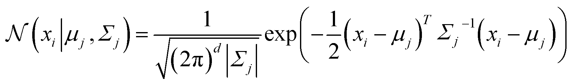 | (21) |
The EM algorithm is used to estimate the parameters {πj, μj, Σj}kj=1 using Expectation (E) and Maximization (M) steps. In the E step, the algorithm calculates the likelihood of each data instance belonging to each cluster based on the current model. In the M step, it updates the cluster parameters (such as the importance of each cluster, the centre of each cluster, and how spread out each cluster is) based on these calculated likelihoods. These steps are repeated until the model's parameters stabilise and no longer change significantly.
GMMs offer several advantages in alloy design due to their flexibility in modelling complex clusters and providing probabilistic assignments of data instances to clusters. This approach is particularly useful when dealing with overlapping phases or heterogeneous data, as it allows for a more nuanced representation of cluster memberships. However, the method also comes with drawbacks, including its computational complexity, especially when dealing with large or high-dimensional data sets. Additionally, GMMs are sensitive to the initialisation of parameters, which can lead to convergence on local optima rather than the global optimum. Moreover, the assumption that the underlying data follows a Gaussian distribution may not always be valid in alloy design. If the actual data distribution deviates significantly from a Gaussian distribution, this could lead to poor model performance.
5.3 Density-based
Density-based methods are particularly adept at discovering clusters of arbitrary shapes, making them well-suited for complex materials systems where the distribution of data instances can be highly irregular.234 The most well-known density-based clustering algorithm is DBSCAN (Density-Based Spatial Clustering of Applications with Noise),237 which relies on two key parameters: ε (epsilon), which represents the maximum distance between two points for one to be considered in the neighbourhood of the other, and MinPts, the minimum number of points required to form a dense region, or cluster. The algorithm begins by identifying core instances with the least MinPts points within a radius of ε. The neighbourhood of p is defined as:| Nε(p) = {q ∈ D∣dist(p, q) ≤ ε} | (22) |
Two instances p and q are density-connected if there is an instance o such that both p and q are density-reachable from o. The clustering process in DBSCAN starts with an arbitrary p and retrieves all instances that are density-reachable from p. If p is a core point, a cluster is formed. If p is a border point, no points are density-reachable from p, and p is labelled as noise or an outlier. The algorithm continues to iterate over all instances in the data set, forming clusters by merging density-connected components.
Density-based clustering, particularly DBSCAN, offers significant advantages due to its ability to discover clusters of arbitrary shapes and sizes. It is also effective at handling noise and outliers, which are common in experimental alloy data sets. DBSCAN does not require the number of clusters to be specified beforehand, making it suitable for exploratory data analysis. However, DBSCAN has its limitations, including its sensitivity to the choice of parameters (ε and MinPts), which can significantly impact the clustering outcome. Additionally, DBSCAN may struggle with varying densities within the same data set, which can lead to the merging of clusters with different densities or the failure to identify some clusters altogether.
5.4 Connectivity-based
Hierarchical clustering algorithms are connectivity-based and identify a systematic hierarchy of cluster labels for a data set, such that there are l layers in the hierarchy, where l is the number of data instances. Hierarchical clustering is either divisive or agglomeration,238 with divisive methods breaking down large clusters into smaller ones,239 and agglomerative methods building up small clusters into larger ones.240 Agglomerative clustering begins by assigning each instance as an individual cluster and recursively merges them until all data instances are in the same cluster, based on their relative distance in the high dimensional feature space, effectively producing a cluster-tree. The pair of clusters with the smallest distance are merged, with the distance defined with linkage criteria, such as single, average, complete or Ward linkage. An advantage of hierarchical clustering is that the number of clusters, K, does not need to be known in advance. However, the time complexity is high and scales quadratically with the number of instances, N.Ward clustering, also known as Ward's method, is a hierarchical, agglomerative clustering technique that minimizes within-cluster variance by iteratively merging clusters that result in the smallest increase in total variance.241 One of the key strengths of Ward clustering is its tendency to produce clusters of approximately equal size, which can be beneficial in applications where balanced groupings are desired. Additionally, because it focuses on minimizing variance, Ward clustering often yields more compact and well-defined clusters compared to other hierarchical methods.242 However, Ward clustering is computationally intensive, especially for large data sets, because it requires the calculation of distances between all pairs of data instances at each step.243
Connectivity-based clustering, particularly hierarchical clustering, is more interpretable than the alternative, as it allows researchers to see relationships in the data at different levels of detail. While hierarchical clustering can be computationally demanding, this is less of an issue for alloy data sets, which are typically not very large. However, the results can vary depending on the chosen linkage method, which can affect how the clusters are formed.
5.5 Graph-based
Graph-based clustering is used when the structure of data can be represented as a network of interconnected points. In graph-based clustering, the data is represented as a graph G = (V, E), where V is a set of vertices (nodes) corresponding to the data instances, and E is a set of edges that represent the relationships or similarities between these points. The weight of an edge typically indicates the strength of the relationship, with higher weights signifying stronger similarities. The goal of graph-based clustering is to partition the graph into subgraphs or clusters such that the nodes within each cluster are more densely connected to each other than to nodes in other clusters. This results in groups of data instances that are highly similar or related according to the graph structure. Common graph-based clustering methods include Spectral Clustering,244 Minimum Spanning Tree (MST) clustering,245,246 and Highly Connected Subgraphs (HCS).229Spectral clustering244 is one of the most widely used graph-based algorithms. It uses a spectrum of eigenvalues of the similarity matrix as a quantitative assessment of the relative similarity of each pair of points in the data set, even if the input is not a graph. The similarity matrix may be defined as a symmetric matrix A, where Aij ≥ 0 measures the similarity between instances i and j. Clustering is applied to the eigenvectors of a Laplacian matrix of A, using the smallest eigenvalues that meet this condition. Spectral clustering is particularly useful for non-convex data or when data can not easily be described by the location of the centroid and the size, shape and density of the surrounding data instances.
Spectral clustering is highly effective for identifying clusters in data that are non-convex or irregularly shaped, where traditional methods like k-Means may fail. By operating in a reduced-dimensional space, it can reveal the underlying structure of the data that might not be apparent in the original feature space. However, the method has some drawbacks, including its computational intensity, especially in the eigenvalue decomposition step, which can be challenging for very large data sets. Additionally, spectral clustering requires a well-defined similarity matrix, and the quality of clustering results heavily depends on how this matrix is constructed. Choosing the right parameters for the similarity matrix can be non-trivial and may require domain-specific knowledge.
5.6 Evaluating clustering results
Evaluating clustering results can be challenging due to the absence of a ground truth, but it is an important step to ensure the predictions are reliable. One of the most convenient ways of doing this is to calculate the ESV,247 as described above, but there are a number of other metrics available to evaluate the performance of clustering algorithms. The silhouette score (S, or silhouette coefficient)248 is a metric used to calculate the consistency of a clustering result, reported in the range from −1 to 1, such that for each data instance: | (23) |
The Davies–Bouldin score (DB)249 is defined as the average similarity measure of each cluster with its most similar cluster, reporting values greater than 0, where similarity is expressed as the ratio of within-cluster distances to between-cluster distances, such that:
 | (24) |
The Calinski–Harabasz score (CH, also referred to as the Variance Ratio Criterion, VRC)250 evaluates the optimal number of clusters based on the variance, such that:
 | (25) |
An alternative way to evaluate clustering outcomes is to use a semi-supervised method such as iterative label spreading, as discussed in Section 7.1.
5.7 Clustering in alloy design
Clustering methods have been used to uncover underlying patterns in a m number of alloy data sets.139,141,149,154,251 In Al6xxx alloys, the k-Means algorithm was used for clustering data following feature reduction via PCA,149 leading to the identification of five distinct groups (as shown in Fig. 6). The impact of feature variations within these clusters on the alloys' properties was analysed using model-agnostic explanation methods, such as the LIME algorithm.253 This analysis revealed a negative influence of the Mg![[thin space (1/6-em)]](https://www.rsc.org/images/entities/char_2009.gif) :Si ratio on mechanical properties, attributed to the formation of Mg2Si precipitates. This relationship would have been obscured during a general regression analysis.
:Si ratio on mechanical properties, attributed to the formation of Mg2Si precipitates. This relationship would have been obscured during a general regression analysis.
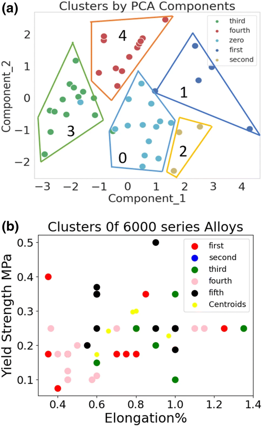 | ||
| Fig. 6 k-Means clustering with PCA (a) and without PCA (b). The plot in (a) demonstrates the benefits of combining k-Means with PCA, resulting in more distinct clusters compared to using k-Means alone. Reproduced from ref. 252, with permission from Springer Nature, Creative Commons Attribution 4.0. | ||
In a Mg alloys corrosion data set, k-Means clustering produced more distinct and separable clusters compared to affinity propagation and hierarchical clustering, as evaluated by scoring metrics such as the silhouette score, Calinski–Harabasz index, and Davies–Bouldin index.154 The k-Means algorithm identified 8 clusters within the data set. Further analysis revealed that two of these clusters were characterised by high Icorr and Ecorr values. Specifically, Fe was found to contribute to corrosion in the alloys of cluster 1, while the presence of Cl was identified as a contributing factor to corrosion in cluster 2. Once again, while a general regression analysis may have uncovered these underlying factors, the clustering is instrumental in showing that they are likely separate mechanisms affecting different alloys rather than simply two influential base metals.
k-Means clustering was used to analyse local variable attributions in the phase classification of multi-principal element alloys (MPEAs) using a support vector machine.139,141 Notably, cluster-specific feature importance differed significantly from global feature importance. This distinction is crucial because relying solely on global importance can obscure variables that are critical for predicting specific phases, potentially leading to misleading conclusions in multi-class classification tasks. Integrating cluster-specific insights ensures a more accurate and targeted MPEA design.
Other clustering algorithms have seen more limited use in alloy design. DBSCAN has been applied to cluster Kinetic Monte-Carlo simulation data of Al–Sc alloys, effectively identifying Sc atoms not belonging to precipitates as outliers, which were then removed before further analysis.254 The dendrogram resulting from the hierarchical clustering of HEAs, illustrated in Fig. 7, highlighted that stacking fault energy (SFE) is strongly influenced by the Rule of Mixtures (RoM) values for formation enthalpy, density, and electronegativity.255 Graph-based clustering methods, such as spectral clustering, have not yet been applied to alloy design. However, they have been effectively utilised to cluster polymers.256–258 For example, spectral clustering successfully identified meta-stable and transition states in polymer molecular dynamics simulations. A similar approach could be employed in alloy research to identify meta-stable precipitates. Other potential applications in alloy research include microstructure analysis and the identification of compositional clusters.
 | ||
| Fig. 7 Dendrogram illustrating the hierarchical clustering of features used in predicting stacking fault energies in high entropy alloys. Reproduced from ref. 255, with permission from Elsevier, Copyright (2023). | ||
6 Outlier detection
Outlier detection is used to identify data instances that deviate significantly from the majority of the data. These outliers can provide crucial insights, reveal errors,259 or indicate novel phenomena.260 An outlier is an observation that lies at an unusually large distance from the central tendency or distribution of other values in a data set.261 If xi is a data instance and μ and σ represent the mean and standard deviation of the data set, respectively, then an outlier is typically defined as a data instance where the distance |xi − μ| exceeds a threshold, such as kσ, where k is a constant:| |xi − μ| > kσ | (26) |
Outliers can be classified into three types: global outliers (also known as point outliers),262 which deviate significantly from the rest of the data set; contextual outliers,263 which are considered outliers in a specific context but not necessarily in the general data set; and collective outliers,261 which are a collection of data instances that collectively deviate from the rest of the data set, even if individual points within the group may not be outliers.
The detection of outliers involves different techniques depending on the type of outlier. Global outliers are typically identified using statistical methods, such as z-scores264 or Tukey's fences,265 which flag data instances that significantly deviate from the mean or median. Contextual outliers require understanding the specific context or conditions that define normal behaviour; they are often detected using techniques like clustering266 or time-series analysis,267 or methods such as RANSAC (Random Sample Consensus),268 which iteratively fits models to subsets of the data and identifies outliers as those points that do not conform to the best model. Collective outliers are more complex and are usually detected through density-based methods,269 or graph-based approaches,270 which analyse the relationships and collective behaviour of data instances.
6.1 Outlying alloys
ML-based outlier detection methods have been employed to identify shear transformation zones (STZs) in amorphous alloys, which are challenging to detect experimentally due to their transient nature.130 Among the methods tested, linear RANSAC proved to be the most accurate in identifying these outliers.Unsupervised learning techniques have also been applied to identify outliers, as shown in Fig. 8, in data sets of ferritic-martensitic steels and austenitic stainless steels.113 Initially, the data set was clustered using PCA and the k-Means algorithm. Outliers were then identified using the Z-score, calculated as:
 | (27) |
 | ||
| Fig. 8 Visualisation of the two largest principal components of the austenitic stainless steel data set with k-Means clustering applied, indicated by crosses representing cluster centres. (b) Outliers in the data set are detected using two approaches: the z-score method. Reproduced from ref. 113, with permission from Springer Nature, Copyright (2022). | ||
7 Semi-supervised learning
Semi-supervised learning (SSL) is a machine learning field that combines supervised and unsupervised learning.274 It uses a small amount of labelled data alongside a larger pool of unlabelled data to improve model performance. The core idea behind SSL is that unlabelled data, when combined with a small amount of labelled data, can greatly improve the learning process.275 SSL works on the assumption that the unlabelled data contains useful information about the structure of the data distribution, which can help improve the accuracy of predictions.274 Several methods are used in SSL, such as self-training, where the model labels unlabelled data and retrains itself; co-training, which involves multiple models working together to label the data; and graph-based methods, which use the relationships between data instances to spread labels across the data set. This approach is particularly valuable when labelling data is costly or time-consuming, as is often the case in materials science.276,2777.1 Iterative label spreading
Iterative label spreading (ILS)278 is a semi-supervised clustering algorithm, based on a general definition of a cluster and the quality of a clustering result, and is capable of predicting the number and type of clusters and outliers in advance of clustering, regardless of the complexity of the distribution of the data.131,279,280 ILS can be used to evaluate the results from other clustering algorithms or perform clustering directly. It has been shown to be more reliable than alternative approaches for simple and challenging cases (such as the null and chain cases) and to be ideal for studying noisy data with high dimensionality and high variance, as is typical for alloys.Direct clustering is achieved using this algorithm by initializing one labelled instance and applying ILS to obtain the ordered minimum distance (Rmin(i)) plot, as described in detail in ref. 279. The number of clusters can be automatically extracted by identifying peaks in the Rmin(i) plot (due to density drops between clusters) that divide the plot into n regions. This can be automated using a continuous wavelet transform peak finding algorithm with smoothing over p points. The smoothing essentially sets the minimum cluster size to identify clusters of no smaller than p. Alternatively, if clear peaks are present, they can be identified easily by visual inspection. One instance can be relabelled in each region (preferably in a dense region, i.e. several grouped minima) to run ILS again and obtain a fully labelled data set with n clusters defined. ILS can also be applied to each individual cluster to confirm that each region is a single cluster that should not be divided further.
7.2 Semi-supervised learning of alloys
ILS has previously been applied to both metallic particles and Al6xxx alloys. It has been used to distinguish between two separable clusters in Pt nanoparticles, with one cluster comprising exclusively disordered nanoparticles and the other containing only ordered nanoparticles.128 In aluminium alloys ILS identified six clusters, as illustrated in Fig. 9a, and was then able to identify further sub-clusters on a second pass, as depicted in Fig. 9b. On analysing the alloys within these clusters, it was observed that their mechanical properties varied within certain ranges. This suggests that specific clusters could be used for optimisation when the target mechanical properties are known. The clusters were subsequently demonstrated to be separable classes using a decision tree classifier.281 The novel classes identified through ILS were then used to enhance the accuracy of forward predictions by training class-specific regressors.282 Further optimisation with these class-specific regressors led to improved aluminium alloy designs compared to a class-agnostic approach.283 Applying similar workflows to other alloy systems remains an area for future investigation.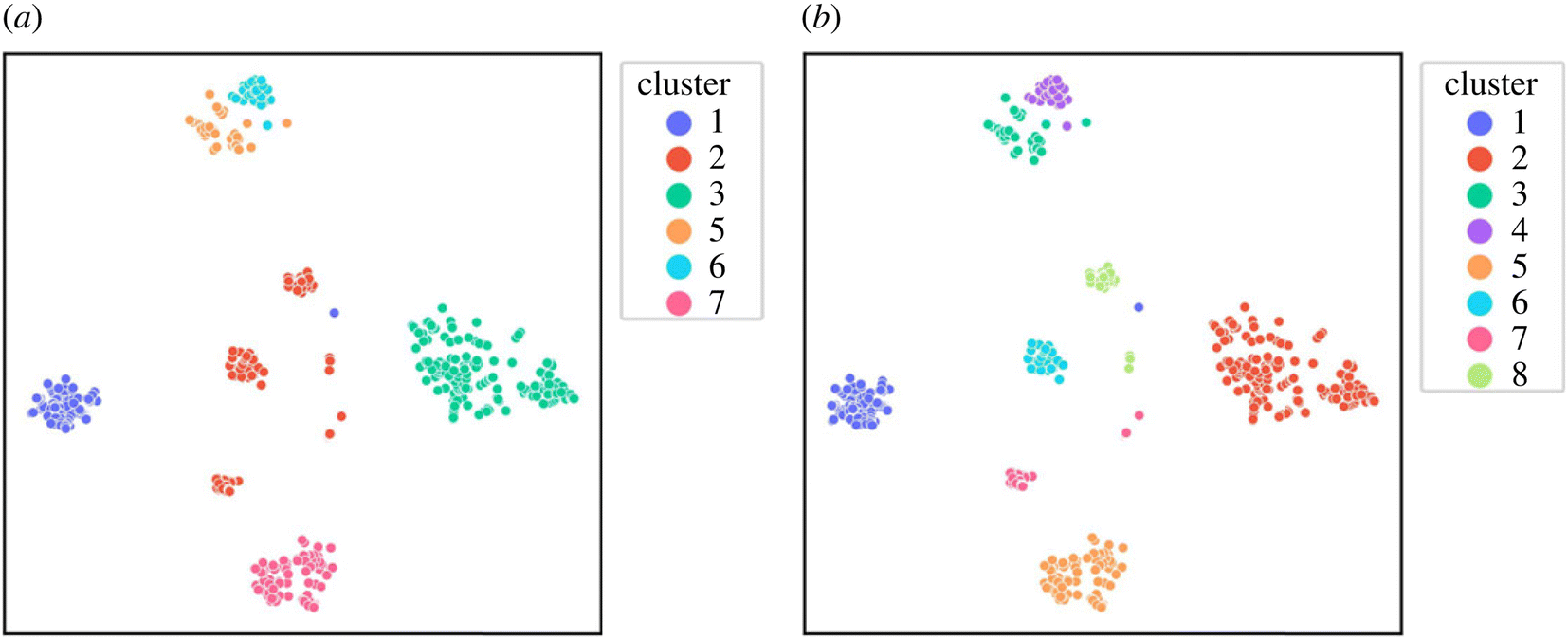 | ||
| Fig. 9 Identification of clusters using Iterative Label Spreading (ILS): (a) clusters identified during the first iteration of ILS, and (b) clusters identified during the second iteration of ILS applied to each sub-cluster. Reproduced from ref. 145, with permission from Royal Society, Creative Commons Attribution License. | ||
8 Summary and opportunities
This brief review suggests that the use of unsupervised methods in alloy design is on the rise, but researchers may not be taking full advantage of these methods. To date the majority of unsupervised learning for alloy design has focused on preparing the data for more effectively supervised learning (such as transforming elemental features into principle components), or capturing established domain knowledge (such as visualising distributions using manifold learning). With the increase in data available, there are more opportunities to use unsupervised machine learning methods than supervised learning, without the added expense of measuring properties. While machine learning is currently widely employed for tasks such as dimensionality reduction and clustering, the community has yet to venture beyond the most simple approaches. Manifold learning, outlier detection, and semi-supervised learning are all under-explored. This presents significant opportunities for further research and innovation in these areas.Based on this summary, research in alloy design should focus on exploring the use of more sophisticated methods to identify deeper relationships between alloys before moving to property prediction or inverse design.145,162 Recent research has demonstrated that the use of clusters identified through ML can partition the data into more predictable groups and significantly improve the accuracy of the model for aluminium alloys.282 Optimising alloy design within smaller clusters is a more sustainable approach compared to optimising alloys in the entire search space, as it reduces redundancy and focuses the models on metals and characteristics that have greater utility in the domain. Additionally, future opportunities also include enhancing data integration and diversity, using a broader range of alloy compositions and processing conditions; and development of advanced unsupervised algorithms specifically tailored for the complexities of alloy systems. This includes algorithms capable of handling multi-scale284 and multi-modal data,285 as well as those that can better capture the non-linear relationships and high-dimensional interactions that characterise alloy behaviour. The emergence of novel methods in computer science will also open up new opportunities, including unsupervised representation learning286 (evidenced by the rise of large language models287), deep clustering algorithms that use neural networks to learn latent representations of data that improve cluster assignment, graph-based unsupervised learning288,289 and unsupervised domain adaptation290 using methods in adversarial learning.291 Self-supervised learning could bridge the gap between supervised and unsupervised learning,292–294 by leveraging methods such as contrastive learning which focuses on learning by comparing data samples.295–297 There is also the potential of exploring hybrid models that combine unsupervised learning with other approaches to further enhance discovery and optimisation processes in alloy design.
Data availability
No data was generated or used as part of this review.Conflicts of interest
There are no conflicts of interest to declare.Acknowledgements
The authors would like to acknowledge useful discussions with Marzie Ghorbani and Zhipeng Li.Notes and references
- S. Ramakrishna, T.-Y. Zhang, W.-C. Lu, Q. Qian, J. S. C. Low, J. H. R. Yune, D. Z. L. Tan, S. Bressan, S. Sanvito and S. R. Kalidindi, J. Intell. Manuf., 2018, 30, 2307–2326 CrossRef.
- G. R. Schleder, A. C. M. Padilha, C. M. Acosta, M. Costa and A. Fazzio, J. Phys.: Mater., 2019, 2, 032001 Search PubMed.
- D. Morgan and R. Jacobs, Annu. Rev. Mater. Res., 2020, 50, 71–103 CrossRef.
- B. Lu, Y. Xia, Y. Ren, M. Xie, L. Zhou, G. Vinai, S. A. Morton, A. T. S. Wee, W. G. van der Wiel, W. Zhang and P. K. J. Wong, Advanced Science, 2024, 11, 2305277 CrossRef PubMed.
- H. Durrant-Whyte, Nat. Rev. Mater., 2021, 6, 641 CrossRef.
- T. Zhou, Z. Song and K. Sundmacher, Engineering, 2019, 5, 1017–1026 CrossRef.
- M. A. El Mrabet, K. El Makkaoui and A. Faize, 2021 4th International Conference on Advanced Communication Technologies and Networking (CommNet), 2021, pp. 1–10 Search PubMed.
- I. H. Sarker, SN Comput. Sci., 2021, 2, 160 CrossRef PubMed.
- R. Vasudevan, G. Pilania and P. V. Balachandran, J. Appl. Phys., 2021, 129, 070401 CrossRef CAS.
- Z. Li, J. Yoon, R. Zhang, F. Rajabipour, W. V. S. III, I. Dabo and A. Radlińska, npj Comput. Mater., 2022, 8, 1–17 CrossRef.
- J. E. Gubernatis and T. Lookman, Phys. Rev. Mater., 2018, 2, 120301 CrossRef CAS.
- J. Schmidt, M. R. G. Marques, S. Botti and M. A. L. Marques, npj Comput. Mater., 2019, 5, 1–36 CrossRef.
- T. Zhou, Z. Song and K. Sundmacher, Engineering, 2019, 5, 1017–1026 CrossRef CAS.
- G. Huang, Y. Guo, Y. Chen and Z. Nie, Materials, 2023, 16, 5977 CrossRef CAS PubMed.
- F. Tanaka, H. Sato, N. Yoshii and H. Matsui, 2018 International Symposium on Semiconductor Manufacturing (ISSM), 2018, pp. 1–3 Search PubMed.
- A. Pratap and N. Sardana, Mater. Today: Proc., 2022, 62, 7341–7347 Search PubMed.
- J. Wei, X. Chu, X. Sun, K. Xu, H.-X. Deng, J. Chen, Z. Wei and M. Lei, InfoMat, 2019, 1, 338–358 CrossRef CAS.
- S. Hong, C. Liow, J. M. Yuk, H. R. Byon, Y. Yang, E. Cho, J. Yeom, G. Park, H. Kang, S. Kim, Y. S. Shim, M. Na, C. Jeong, G. Hwang, H. Kim, H. Kim, S. Eom, S. Cho, H. Jun, Y. Lee, A. Baucour, K. Bang, M. Kim, S. Yun, J. Ryu, Y. Han, A. Jetybayeva, P. Choi, J. C. Agar, S. V. Kalinin, P. W. Voorhees, P. Littlewood and H.-M. Lee, ACS Nano, 2021, 15, 3971–3995 CrossRef CAS PubMed.
- W. F. Maier, K. Stöwe and S. Sieg, Angew. Chem., 2007, 46, 6016–6067 CrossRef CAS PubMed.
- A. Ludwig, npj Comput. Mater., 2019, 5, 1–7 CrossRef.
- L. Zhao, Y. Zhou, H. Wang, X. Chen, L. Yang, L. Zhang, L. Jiang, Y. H. Jia, X. Chen and H. Wang, Metall. Mater. Trans. A, 2021, 52, 1159–1168 CrossRef CAS.
- J. Gregoire, L. Zhou and J. A. Haber, Nat. Synth., 2023, 2, 493–504 CrossRef.
- K. Shahzad, A. I. Mardare and A. W. Hassel, Sci. Technol. Adv. Mater.: Methods, 2024, 4, 2292486 Search PubMed.
- W. L. Ng, G. L. Goh, G. D. Goh, J. S. J. Ten and W. Y. Yeong, Adv. Mater., 2024, 36, 2310006 CrossRef CAS.
- Y. B. Baris Ördek and E. Coatanea, Prod. Manuf. Res., 2024, 12, 2326526 Search PubMed.
- A. Tran, J. Tranchida, T. Wildey and A. P. Thompson, J. Chem. Phys., 2020, 153 7, 074705 CrossRef.
- T. Mueller, A. G. Kusne and R. Ramprasad, Rev. Comput. Chem., 2016, 186–273 Search PubMed.
- B. Sun, M. Fernandez and A. S. Barnard, Nanoscale Horiz., 2016, 1, 89–95 RSC.
- A. S. Barnard, B. Motevalli, A. J. Parker, J. M. Fischer, C. A. Feigl and G. Opletal, Nanoscale, 2019, 11, 19190–19201 RSC.
- H. Yin, Z. Sun, Z. Wang, D. Tang, C. H. Pang, X. Yu, A. S. Barnard, H. Zhao and Z. Yin, Cell Rep. Phys. Sci., 2021, 2, 100482 CrossRef.
- S. Li and A. S. Barnard, Adv. Theory Simul., 2021, 5, 2100414 CrossRef.
- A. Challapalli, D. Patel and G. Li, Mater. Des., 2021, 208, 109937 CrossRef.
- C. S. Ha, D. Yao, Z. Xu, C. Liu, H. Liu, D. Elkins, M. Kile, V. S. Deshpande, Z. Kong, M. Bauchy and X. R. Zheng, Nat. Commun., 2023, 14, 5765 CrossRef CAS PubMed.
- J. Lee, D.-O. Park, M. Lee, H. Lee, K. Park, I. Lee and S. W. Ryu, Mater. Horiz., 2023, 10, 5436–5456 RSC.
- G.-J. Qi and J. Luo, IEEE Trans. Pattern Anal. Mach. Intell., 2019, 44, 2168–2187 Search PubMed.
- R. Ferrando, J. Jellinek and R. L. Johnston, Chem. Rev., 2008, 108(3), 845–910 CrossRef CAS PubMed.
- Y. Wang, L. Zhang, B. Xu, X. Wang and H. Wang, Modell. Simul. Mater. Sci. Eng., 2021, 30, 025003 CrossRef.
- Z. Yang and W. GAO, Advanced Science, 2022, 9, 2106043 CrossRef CAS.
- S. Han, G. Barcaro, A. Fortunelli, S. Lysgaard, T. Vegge and H. A. Hansen, npj Comput. Mater., 2022, 8, 121 CrossRef.
- Q. Gromoff, P. Benzo, W. A. Saidi, C. M. Andolina, M.-J. Casanove, T. Hungria, S. Barre, M. Benoit and J. Lam, Nanoscale, 2024, 16, 384–393 RSC.
- J. Zhang, X. Liu, S. Bi, J. Yin, G. Zhang and M. Eisenbach, Mater. Des., 2020, 185, 108247 CrossRef CAS.
- B. Akhil, A. Bajpai, N. P. Gurao and K. Biswas, Modell. Simul. Mater. Sci. Eng., 2021, 29, 085005 CrossRef CAS.
- L. Li, B. Xie, Q. Fang and J. Li, Metall. Mater. Trans. A, 2021, 52, 439–448 CrossRef CAS.
- A. Pandey, J. G. Gigax and R. Pokharel, JOM, 2022, 74, 2908–2920 CrossRef CAS.
- G. Hayashi, K. Suzuki, T. Terai, H. Fujii, M. Ogura and K. Sato, Sci. Technol. Adv. Mater.: Methods, 2022, 2, 381–391 CAS.
- X. Liu, J. Zhang and Z. Pei, Prog. Mater. Sci., 2022, 131, 101018 CrossRef.
- Z. Rao, P.-Y. Tung, R. Xie, Y. Wei, H. Zhang, A. Ferrari, T. P. C. Klaver, F. Körmann, P. T. Sukumar, A. K. da Silva, Y. Chen, Z. Li, D. Ponge, J. Neugebauer, O. Gutfleisch, S. Bauer and D. Raabe, Science, 2022, 378, 78–85 CrossRef.
- G. Vazquez, P. K. Singh, D. Sauceda, R. Couperthwaite, N. Britt, K. Youssef, D. D. Johnson and R. Arr’oyave, Acta Mater., 2022, 232, 117924 CrossRef.
- Y. Zeng, M. Man, C. K. Ng, D. Wuu, J. J. Lee, F. Wei, P. Wang, K. Bai, D. C. C. Tan and Y.-W. Zhang, APL Mater., 2022, 10, 101104 CrossRef.
- S. Kamnis, A. K. Sfikas and S. González, International Thermal Spray Conference, 2022, pp. 522–533 Search PubMed.
- U. Bhandari, M. R. Rafi, C. Zhang and S. Yang, Mater. Today Commun., 2020, 101871 Search PubMed.
- J. Wang, H. Kwon, H. S. Kim and B. J. Lee, npj Comput. Mater., 2023, 9, 1–13 CrossRef.
- M. Kandavalli, A. Agarwal, A. Poonia, M. Kishor and K. P. R. Ayyagari, Sci. Rep., 2023, 13, 20504 CrossRef.
- S. Liu and C. Yang, Metals, 2024, 14, 235 CrossRef CAS.
- A. B. Mazitov, M. A. Springer, N. Lopanitsyna, G. Fraux, S. De and M. Ceriotti, J. Phys.: Mater., 2023, 7, 025007 Search PubMed.
- J. Berry, R. M. Snell, M. Anderson, L. R. Owen, O. M. Messé, I. Todd and K. A. Christofidou, Adv. Eng. Mater., 2024, 26, 2302064 CrossRef CAS.
- S. Zhao, R. Yuan, W. Liao, Y. Zhao, J. Wang, J. Li and T. Lookman, J. Mater. Chem. A, 2024, 12, 2807–2819 RSC.
- S.-H. V. Oh, S.-H. Yoo and W. Jang, npj Comput. Mater., 2024, 10, 1–7 CrossRef.
- P. Rambabu, N. Eswara Prasad, V. Kutumbarao and R. Wanhill, Aerospace Materials and Material Technologies: Volume 1: Aerospace Materials, 2017, pp. 29–52 Search PubMed.
- R. Boyer, Adv. Perform. Mater., 1995, 2, 349–368 CrossRef CAS.
- M. K. Kulekci, Int. J. Adv. Des. Manuf. Technol., 2008, 39, 851–865 CrossRef.
- W. Miller, L. Zhuang, J. Bottema, A. Wittebrood, P. De Smet, A. Haszler and A. Vieregge, Mater. Sci. Eng. A, 2000, 280, 37–49 CrossRef.
- M. A. Wahid, A. N. Siddiquee and Z. A. Khan, Mar. Syst. Ocean Technol., 2020, 15, 70–80 CrossRef.
- R. Willms, Nordic Steel Construction Conference, Malmo, Sweden, 2009 Search PubMed.
- S. Magdassi, M. Grouchko and A. Kamyshny, Materials, 2010, 3, 4626–4638 CrossRef CAS PubMed.
- J. S. Faulkner, Prog. Mater. Sci., 1982, 27, 1–187 CrossRef CAS.
- F. Habashi, Alloys: Preparation, Properties, Applications, John Wiley & Sons, 2008 Search PubMed.
- K.-E. Thelning, Steel and its Heat Treatment, Butterworth-Heinemann, 1975, pp. 82–126 Search PubMed.
- J. Westbrook, Computerization and Networking of Materials Data Bases, ASTM International, 1989 Search PubMed.
- P. K. Samal, Powder Metallurgy, ASM International, 2015, pp. 415–420 Search PubMed.
- I. Polmear, D. StJohn, J.-F. Nie and M. Qian, Light Alloys: Metallurgy of the Light Metals, Butterworth-Heinemann, 2017 Search PubMed.
- J. G. Kaufman, in Understanding Wrought and Cast Aluminum Alloy Designations, ASM International, 2013, pp. 23–37 Search PubMed.
- J. Christian, The Theory of Transformations in Metals and Alloys, Newnes, 2002 Search PubMed.
- H. J. Goldschmid, Interstitial alloys, Springer, 2013 Search PubMed.
- D. S. Thompson, Metall. Trans. A, 1975, 6, 671–683 CrossRef.
- G. S. Upadhyaya, Powder Metallurgy Technology, Cambridge Int Science Publishing, 1997 Search PubMed.
- L. Sun, G. Yuan, L. Gao, J. Yang, M. Chhowalla, M. H. Gharahcheshmeh, K. K. Gleason, Y. S. Choi, B. H. Hong and Z. Liu, Nat. Rev. Methods Primers, 2021, 1, 5 CrossRef.
- J. C.-M. Li, Microstructure and properties of materials, World Sci., 1996, 2, 1–452 Search PubMed.
- V. B. Ginzburg, Steel-Rolling Technology: Theory and Practice, CRC Press, 1989 Search PubMed.
- H. Yoshimura and K. Tanaka, J. Mater. Process. Technol., 2000, 98, 196–204 CrossRef.
- D. Edmonds, K. He, F. Rizzo, B. De Cooman, D. Matlock and J. Speer, Mater. Sci. Eng. A, 2006, 438, 25–34 CrossRef.
- I. Polmear and M. Couper, Metall. Trans. A, 1988, 19, 1027–1035 CrossRef.
- A. Abu-Odeh, E. Galvan, T. Kirk, H. Mao, Q. Chen, P. Mason, R. Malak and R. Arróyave, Acta Mater., 2018, 152, 41–57 CrossRef.
- X. Yang, G. M. El-Fallah, Q. Tao, J. Fu, C. Leng, J. Shepherd and H. Dong, Mater. Today Commun., 2023, 34, 105162 CrossRef.
- R. O. Ritchie, Nat. Mater., 2011, 10, 817–822 CrossRef PubMed.
- J. L. Cann, A. De Luca, D. C. Dunand, D. Dye, D. B. Miracle, H. S. Oh, E. A. Olivetti, T. M. Pollock, W. J. Poole and R. Yang, et al. , Prog. Mater. Sci., 2021, 117, 100722 CrossRef CAS.
- A. Aversa, G. Marchese, A. Saboori, E. Bassini, D. Manfredi, S. Biamino, D. Ugues, P. Fino and M. Lombardi, Materials, 2019, 12, 1007 CrossRef CAS PubMed.
- Y. Kong, Z. Jia, Z. Liu, M. Liu, H. J. Roven and Q. Liu, J. Alloys Compd., 2021, 857, 157611 CrossRef.
- N. Gaudence, N. Aimable, T. Mbuya and B. Mose, International Journal of Engineering Research & Technology, 2019, 8, bIJERTV8IS050281 Search PubMed.
- R. Kaçar and K. Güleryüz, Mater. Res., 2015, 18, 328–333 CrossRef.
- A. V. Lozhnikova, P. P. Shchetinin, N. Skrylnikova and N. Redchikova, Key Eng. Mater., 2016, 683, 15–21 Search PubMed.
- V. Zackay, E. Parker, J. Morris Jr and G. Thomas, Mater. Sci. Eng., 1974, 16, 201–221 CrossRef.
- M. J. Donachie and S. Donachie, Mechanical Engineers Handbook, 2015, vol. 299 Search PubMed.
- T. M. Pollock and A. Van der Ven, MRS Bull., 2019, 44, 238–246 CrossRef.
- G. L. Hart, T. Mueller, C. Toher and S. Curtarolo, Nat. Rev. Mater., 2021, 6, 730–755 CrossRef.
- M. Hu, Q. Tan, R. Knibbe, M. Xu, B. Jiang, S. Wang, X. Li and M.-X. Zhang, Mater. Sci. Eng. R: Rep., 2023, 155, 100746 CrossRef.
- E. Swann, B. Sun, D. Cleland and A. Barnard, Mol. Simul., 2018, 44, 905–920 CrossRef.
- V. Tshitoyan, J. Dagdelen, L. Weston, A. Dunn, Z. Rong, O. Kononova, K. A. Persson, G. Ceder and A. Jain, Nature, 2019, 571, 95–98 CrossRef CAS PubMed.
- C. Sammut and G. I. Webb, in Clustering, Springer US, Boston, MA, 2010, p. 180 Search PubMed.
- S. Velliangiri, S. Alagumuthukrishnan and S. I. T. joseph, Procedia Comput. Sci., 2019, 165, 104–111 CrossRef.
- B. Motevalli, A. J. Parker, B. Sun and A. S. Barnard, Nano Futures, 2019, 3, 045001 CrossRef.
- R. Ouyang, S. Curtarolo, E. Ahmetcik, M. Scheffler and L. M. Ghiringhelli, Phys. Rev. Mater., 2018, 2, 083802 CrossRef.
- M. A. Bessa, R. Bostanabad, Z. Liu, A. Hu, D. W. Apley, C. Brinson, W. Chen and W. K. Liu, Comput. Methods Appl. Mech. Eng., 2017, 320, 633–667 CrossRef.
- M. Wenzlick, O. Mamun, R. Devanathan, K. Rose and J. Hawk, J. Mater. Eng. Perform., 2021, 30, 823–838 CrossRef.
- R. Bellman, Introduction to the mathematical theory of control processes: Linear equations and quadratic criteria, Elsevier, 2016 Search PubMed.
- X. Huang, L. Wu and Y. Ye, Int. J. Pattern Recognit. Artif. Intell., 2019, 33, 1950017 CrossRef.
- R. Jha, G. S. Dulikravich, N. Chakraborti, M. Fan, J. Schwartz, C. C. Koch, M. J. Colaco, C. Poloni and I. N. Egorov, Mater. Manuf. Processes, 2017, 32, 1067–1074 CrossRef.
- I. Toda-Caraballo, E. I. Galindo-Nava and P. E. Rivera-Díaz-del Castillo, J. Alloys Compd., 2013, 566, 217–228 CrossRef.
- J. P. Stevens, Psychol. Bull., 1984, 95, 334 Search PubMed.
- E. Acuña and C. Rodriguez, in A Meta analysis study of outlier detection methods in classification, University of Puerto Rico at Mayaguez, 2004, vol. 15 Search PubMed.
- T. Liu, Z. Y. Tho and A. S. Barnard, Digital Discovery, 2024, 3, 422–435 RSC.
- L. Tian, Y. Fan, L. Li and N. Mousseau, Scr. Mater., 2020, 186, 185–189 CrossRef CAS.
- M. Wenzlick, O. Mamun, R. Devanathan, K. Rose and J. Hawk, Jom, 2022, 74, 2846–2859 CrossRef.
- G. L. W. Hart, T. Mueller, C. Toher and S. Curtarolo, Nat. Rev. Mater., 2021, 6, 730–755 CrossRef.
- J. F. Durodola, Prog. Mater. Sci., 2021, 100797 Search PubMed.
- X. Liu, P. Xu, J. Zhao, W. Lu, M. Li and G. Wang, J. Alloys Compd., 2022, 921, 165984 CrossRef CAS.
- H. Fu, H. Zhang, C. Wang, W. Yong and J.-X. Xie, Int. J. Miner., Metall. Mater., 2022, 29, 635–644 CrossRef CAS.
- M. Hu, Q. Tan, R. Knibbe, M. Xu, B. Jiang, S. Wang, X. Li and M. Zhang, Mater. Sci. Eng. R: Rep., 2023, 155, 100746 CrossRef.
- B. Sun, M. Fernández and A. S. Barnard, J. Chem. Inf. Model., 2017, 57(10), 2413–2423 CrossRef CAS PubMed.
- A. S. Mangsor, Z. H. Rizvi, K. T. Chaudhary and M. S. Aziz, J. Phys.: Conf. Ser., 2018, 1027, 012017 CrossRef.
- B. Sun and A. S. Barnard, J. Phys.: Mater., 2018, 1, 016001 Search PubMed.
- A. A. Shirinyan, V. K. Kozin, J. Hellsvik, M. Pereiro, O. Eriksson and D. Yudin, Phys. Rev. B, 2019, 99, 041108 CrossRef.
- A. K. Verma, W.-H. Huang, J. A. Hawk, L. S. Bruckman, R. H. French, V. Romanov and J. L. Carter, Mater. Sci. Eng. A, 2019, 763, 138142 CrossRef.
- R. Jha and G. S. Dulikravich, Metals, 2019, 9, 537 CrossRef.
- N. Krishnamurthy, S. Maddali, J. A. Hawk and V. N. Romanov, Comput. Mater. Sci., 2019, 168, 268–279 CrossRef.
- A. K. Verma, J. A. Hawk, L. S. Bruckman, R. H. French, V. Romanov and J. L. Carter, Metall. Mater. Trans. A, 2019, 50, 3106–3120 CrossRef.
- B. Sun and A. S. Barnard, J. Phys.: Mater., 2019, 2, 034003 Search PubMed.
- A. J. Parker, G. Opletal and A. S. Barnard, J. Appl. Phys., 2020, 128, 014301 CrossRef CAS.
- A. Dasgupta, Y. Gao, S. R. Broderick, E. B. Pitman and K. Rajan, J. Phys. Chem. C, 2020, 124, 14158–14166 CrossRef CAS.
- L. Tian, Y. Fan, L. Li and N. Mousseau, Scr. Mater., 2020, 186, 185–189 CrossRef CAS.
- A. J. Parker, B. Motevalli, G. Opletal and A. S. Barnard, Nanotechnology, 2020, 32, 095404 CrossRef.
- J. A. Esterhuizen, B. R. Goldsmith and S. Linic, Chem Catal., 2021, 1, 923–940 CrossRef CAS.
- J. Jung, J. I. Yoon, H. K. Park, H. Jo and H. S. Kim, Materialia, 2020, 11, 100690 CrossRef.
- C. Liu, E. Fujita, Y. Katsura, Y. Inada, A. Ishikawa, R. Tamura, K. Kimura and R. Yoshida, Adv. Mater., 2021, 33, 2102507 CrossRef CAS.
- J. A. Esterhuizen, B. R. Goldsmith and S. Linic, Chem Catal., 2021, 1, 923–940 CrossRef CAS.
- R. Subbarao, et al. , Mater. Today: Proc., 2021, 46, 8615–8620 Search PubMed.
- Y. Kim, H. K. Park, J. Jung, P. Asghari-Rad, S. Lee, J. Y. Kim, H. G. Jung and H. S. Kim, Mater. Des., 2021, 202, 109544 CrossRef.
- J. Yin, Z. Pei and M. C. Gao, Nat. Comput. Sci., 2021, 1, 686–693 CrossRef PubMed.
- K. Lee, M. V. Ayyasamy, P. Delsa, T. Q. Hartnett and P. V. Balachandran, npj Comput. Mater., 2022, 8, 25 CrossRef.
- S. Chintakindi, A. Alsamhan, M. H. Abidi and M. P. Kumar, Int. J. Comput. Intell. Syst., 2022, 15, 18 CrossRef.
- K. Lee, M. V. Ayyasamy, Y. Ji and P. V. Balachandran, Sci. Rep., 2022, 12, 11591 CrossRef PubMed.
- Z. C. Xin, J. S. Zhang, Y. Jin, J. Zheng and Q. Liu, Int. J. Miner., Metall. Mater., 2022, 30, 335–344 CrossRef.
- A. S. Bundela and M. Rahul, Metall. Mater. Trans. A, 2022, 53, 3512–3519 CrossRef.
- A. L. Foggiatto, Y. Mizutori, T. Yamazaki, S. Sato, K. Masuzawa, R. Nagaoka, M. Taniwaki, S. Fujieda, S. Suzuki and K. Ishiyama, et al. , IEEE Trans. Magn., 2023, 59, 2501604 Search PubMed.
- O. Ahmad, N. Kumar, R. Mukherjee and S. Bhowmick, Phys. Rev. Mater., 2023, 7, 083802 CrossRef.
- N. Bhat, A. S. Barnard and N. Birbilis, R. Soc. Open Sci., 2023, 10, 220360 CrossRef.
- M. Ghorbani, M. Boley, P. Nakashima and N. Birbilis, J. Magnesium Alloys, 2023, 11, 3620–3633 CrossRef CAS.
- H.-F. Chen, Y.-P. Yang, W.-L. Chen, P. J. Wang, W. Lai, Y.-K. Fuh and T. T. Li, Mater. Chem. Phys., 2023, 295, 127070 CrossRef.
- T. Tiwari, S. Jalalian, C. L. Mendis and D. G. Eskin, JOM, 2023, 75, 4526–4537 CrossRef.
- J. Y. C. Ting, A. J. Parker and A. S. Barnard, Chem. Mater., 2023, 35, 728–738 CrossRef.
- C. Roncaglia and R. Ferrando, J. Chem. Inf. Model., 2023, 63, 459–473 CrossRef.
- B. Vela, C. Acemi, P. Singh, T. Kirk, W. Trehern, E. Norris, D. D. Johnson, I. Karaman and R. Arróyave, Acta Mater., 2023, 248, 118784 CrossRef.
- S. Fetni, T. Q. D. Pham, T. V. Hoang, H. S. Tran, L. Duchêne, X.-V. Tran and A. M. Habraken, Comput. Mater. Sci., 2023, 216, 111820 CrossRef.
- A. Moses, X. Peng, S. Wang and D. Chen, JOM, 2024, 76, 4388–4403 CrossRef.
- X. Liu, Y. Bao, L. Zhao and C. Gu, J. Sustain. Metall., 2024, 10, 509–524 CrossRef.
- A. Usuga, C. Praveen and A. Comas-Vives, J. Mater. Chem. A, 2024, 12, 2708–2721 RSC.
- B. Venkatesh and J. Anuradha, Cybern. Inf. Technol., 2019, 19, 3–26 Search PubMed.
- C. Yang, C. Ren, Y. Jia, G. Wang, M. Li and W. Lu, Acta Mater., 2022, 222, 117431 CrossRef.
- J. Li, K. Cheng, S. Wang, F. Morstatter, R. P. Trevino, J. Tang and H. Liu, ACM Computing Surveys (CSUR), 2017, 50, 1–45 Search PubMed.
- K. Kira and L. A. Rendell, Machine Learning Proceedings 1992, Elsevier, 1992, pp. 249–256 Search PubMed.
- J. G. Dy and C. E. Brodley, J. Mach. Learn. Res., 2004, 5, 845–889 Search PubMed.
- N. Bhat, A. S. Barnard and N. Birbilis, J. Mater. Sci., 2024, 59, 1448–1463 CrossRef.
- A. Altmann, L. Toloşi, O. Sander and T. Lengauer, Bioinformatics, 2010, 26, 1340–1347 CrossRef PubMed.
- K. V. Priyadharshini, A. Vijay, K. Swaminathan, T. Avudaiappan and V. Banupriya, Mater. Today: Proc., 2022, 69, 710–715 Search PubMed.
- P.-P. D. Breuck, G. Hautier and G. Rignanese, npj Comput. Mater., 2020, 7, 1–8 Search PubMed.
- B. Hoock, S. Rigamonti and C. Draxl, New J. Phys., 2022, 24, 113049 CrossRef.
- H. Abdi and L. J. Williams, Wiley Interdiscip. Rev. Comput. Stat., 2010, 2, 433–459 CrossRef.
- S. Schneider, S. G. Schneider, H. M. d. Silva and C. d. Moura Neto, Mater. Res., 2005, 8, 435–438 CrossRef.
- H. Xu, C. Caramanis and S. Mannor, IEEE Trans. Inf. Theory, 2012, 59, 546–572 Search PubMed.
- K. Rajan, C. Suh and P. F. Mendez, Stat. Anal. Data Min., 2009, 1, 361–371 CrossRef.
- V. Klema and A. J. Laub, IEEE Trans. Autom. Control, 1980, 25, 164–176 CrossRef.
- B. P. Epps and E. M. Krivitzky, Exp. Fluids, 2019, 60, 1–23 CrossRef.
- M. Brand, Computer Vision—ECCV 2002: 7th European Conference on Computer Vision, Copenhagen, Denmark, 2002, pp. 707–720 Search PubMed.
- H. Swathi, S. Sohini, Surbhi and G. Gopichand, IOP Conf. Ser.: Mater. Sci. Eng., 2017, 263, 042082 Search PubMed.
- C. Zhang, R. Han, A. Zhang and P. Voyles, Microsc. Microanal., 2020, 26, 1722–1723 CrossRef.
- A. Cutler and L. Breiman, Technometrics, 1994, 36, 338–347 CrossRef.
- S. Mair and U. Brefeld, 33rd Conference on Neural Information Processing Systems, Vancouver, Canada, 2019 Search PubMed.
- M. Fernandez and A. S. Barnard, ACS Nano, 2015, 9, 11980–11992 CrossRef CAS.
- M. Fernandez, H. F. Wilson and A. S. Barnard, Nanoscale, 2017, 9, 832–843 RSC.
- T. Kohonen, Proc. IEEE, 1990, 78, 1464–1480 CrossRef.
- C. Bishop, Clarendon Press google scholar, 1995, 2, pp. 223–228 Search PubMed.
- A. S. Barnard, B. Motevalli and B. Sun, MRS Commun., 2019, 9, 730–736 CrossRef.
- B. Sun and A. S. Barnard, J. Phys.: Mater., 2018, 1, 016001 Search PubMed.
- P. Wittek, S. C. Gao, I. S. Lim and L. Zhao, arXiv, preprint, arXiv:1305.1422, 2013, DOI:10.18637/jss.v078.i09.
- W. Gardner, R. Maliki, S. M. Cutts, B. W. Muir, D. Ballabio, D. A. Winkler and P. J. Pigram, Anal. Chem., 2020, 92, 10450–10459 CrossRef PubMed.
- S. Y. Wong, S. L. Harmer, W. Gardner, A. K. Schenk, D. Ballabio and P. J. Pigram, Adv. Mater. Interfaces, 2023, 10, 10450–10459 Search PubMed.
- S. E. Bamford, W. Gardner, D. A. Winkler, B. W. Muir, D. Alahakoon and P. J. Pigram, J. Am. Soc. Mass Spectrom., 2024, 35, 2516–2528 CrossRef PubMed.
- D. Bank, N. Koenigstein and R. Giryes, Machine Learning for Data Science Handbook: Data Mining and Knowledge Discovery Handbook, 2023, pp. 353–374 Search PubMed.
- W. Wang, Y. Huang, Y. Wang and L. Wang, Proceedings of the IEEE Conference on Computer Vision and Pattern Recognition Workshops, 2014, pp. 490–497 Search PubMed.
- M. Sakurada and T. Yairi, Proceedings of the MLSDA 2014 2nd Workshop on Machine Learning for Sensory Data Analysis, 2014, pp. 4–11 Search PubMed.
- Q. Meng, D. Catchpoole, D. Skillicom and P. J. Kennedy, 2017 International Joint Conference on Neural Networks (IJCNN), 2017, pp. 364–371 Search PubMed.
- Y. Wang, H. Yao and S. Zhao, Neurocomputing, 2016, 184, 232–242 CrossRef.
- E. Ordway-West, P. Parveen and A. Henslee, 2018 IEEE International Congress on Big Data (BigData Congress), 2018, pp. 205–209 Search PubMed.
- J. Baima, A. M. Goryaeva, T. D. Swinburne, J.-B. Maillet, M. Nastar and M.-C. Marinica, Phys. Chem. Chem. Phys., 2022, 24, 23152–23163 RSC.
- S. Fetni, T. Q. D. Pham, T. V. Hoang, H. S. Tran, L. Duchêne, X.-V. Tran and A. M. Habraken, Comput. Mater. Sci., 2023, 216, 111820 CrossRef.
- A. Choudhury, Y. C. Yabansu, S. R. Kalidindi and A. Dennstedt, Acta Mater., 2016, 110, 131–141 CrossRef.
- A. S. Mangsor, Z. H. Rizvi, K. Chaudhary and M. S. Aziz, J. Phys.: Conf. Ser., 2018, 012017 CrossRef.
- Z. Zhuang and A. S. Barnard, Chem. Mater., 2023, 35, 9325–9338 CrossRef.
- B. Motevalli, A. J. Parker, B. Sun and A. S. Barnard, Nano Futures, 2019, 3, 045001 CrossRef.
- Y. Ji, A. Koeppe, P. Altschuh, D. Rajagopal, Y. Zhao, W. Chen, Y. Zhang, Y. Zheng and B. Nestler, Comput. Mater. Sci., 2024, 232, 112628 CrossRef.
- X. Huo and A. Smith, Series on Computers and Operations Research, in, Recent Advances in Data Mining of Enterprise Data: Algorithms and Applications, 2008, pp. 691–745 Search PubMed.
- J. B. Kruskal, Psychometrika, 1964, 29, 115–129 CrossRef.
- S. T. Roweis and L. K. Saul, Science, 2000, 290(5500), 2323–2326 CrossRef.
- J. B. Tenenbaum, V. de Silva and J. C. Langford, Science, 2000, 290(5500), 2319–2323 CrossRef.
- M. Belkin and P. Niyogi, Neural Comput., 2003, 15, 1373–1396 CrossRef.
- L. McInnes, J. Healy, N. Saul and L. Großberger, J. Open Source Softw., 2018, 3, 861 CrossRef.
- L. van der Maaten, J. Mach. Learn. Res., 2014, 15, 3221–3245 Search PubMed.
- A. S. Barnard and G. Opletal, Nanoscale, 2019, 11, 23165–23172 RSC.
- D. Kobak and G. C. Linderman, Nat. Biotechnol., 2021, 39, 156–157 CrossRef.
- L. Van der Maaten and G. Hinton, J. Mach. Learn. Res., 2008, 9, 2579–2605 Search PubMed.
- L. McInnes, J. Healy, N. Saul and L. Großberger, J. Open Source Softw., 2018, 3, 861 CrossRef.
- E. Becht, L. McInnes, J. Healy, C.-A. Dutertre, I. W. Kwok, L. G. Ng, F. Ginhoux and E. W. Newell, Nat. Biotechnol., 2019, 37, 38–44 CrossRef.
- S. Kim, L. Zhang, S.-H. Kim and Y. S. Choi, Met. Mater. Int., 2024, 30, 1817–1830 CrossRef.
- T. Zhang, R. Ramakrishnan and M. Livny, ACM SIGMOD Conference, 1996, pp. 103–114 Search PubMed.
- M. Wenzlick, O. Mamun, R. Devanathan, K. K. Rose and J. A. Hawk, J. Mater. Eng. Perform., 2021, 1–16 Search PubMed.
- X. Liu, X. Qu, X. Xie, S. Li, Y. Bao and L. Zhao, Processes, 2024, 12, 974 CrossRef.
- K. Li, B. DeCost, K. Choudhary, M. Greenwood and J. Hattrick-Simpers, npj Comput. Mater., 2023, 9, 55 CrossRef.
- A. J. Parker and A. S. Barnard, Nanoscale Horiz., 2020, 5, 1394–1399 RSC.
- A. J. Parker and A. S. Barnard, Nanoscale Horiz., 2021, 6, 277–282 RSC.
- P. Karande, B. Gallagher and T. Y.-J. Han, Chem. Mater., 2022, 34, 7650–7665 CrossRef.
- S. S. Chong, Y. S. Ng, H. Wang and J.-C. Zheng, Front. Phys., 2023, 19, 13501 CrossRef.
- R. Xu and D. Wunsch, IEEE Trans. Neural Netw., 2005, 16, 645–678 CrossRef PubMed.
- A. E. Ezugwu, A. M. Ikotun, O. O. Oyelade, L. Abualigah, J. O. Agushaka, C. I. Eke and A. A. Akinyelu, Eng. Appl. Artif. Intell., 2022, 110, 104743 CrossRef.
- D. Xu and Y. jie Tian, Ann. Data Sci., 2015, 2, 165–193 CrossRef.
- V. V. Romanuke, Decis. Mak.: Appl. Manag. Eng., 2023, 6, 734–746 Search PubMed.
- C. Liu, J. Multivar. Anal., 1999, 69, 206–217 CrossRef.
- M. Ester, H.-P. Kriegel, J. Sander and X. Xu, Knowledge Discovery and Data Mining, 1996, pp. 226 – 231 Search PubMed.
- F. Murtagh and P. Contreras, Wiley Interdiscip. Rev.: Data Min. Knowl. Discov., 2012, 2, 86–97 Search PubMed.
- E. Hartuv and R. Shamir, Inf. Process. Lett., 2000, 76, 175–181 CrossRef.
- T. Xiang and S. Gong, Pattern Recognit., 2008, 41, 1012–1029 CrossRef.
- M.-S. Yang, Math. Comput. Model., 1993, 18, 1–16 CrossRef.
- S. K. Uppada, International Journal of Computer Science and Information Technologies, 2014, 5, 7309–7313 Search PubMed.
- J. MacQueen et al. , Proceedings of the fifth Berkeley symposium on mathematical statistics and probability, 1967, pp. 281–297 Search PubMed.
- D. Xu and Y. Tian, Ann. Data Sci., 2015, 2, 165–193 CrossRef.
- D. A. Reynolds et al. , Encyclopedia of biometrics, 2009, 741 Search PubMed.
- G. Xuan, W. Zhang and P. Chai, Proceedings 2001 International Conference on Image Processing (Cat. No. 01CH37205), 2001, pp. 145–148 Search PubMed.
- M. Ester, H.-P. Kriegel, J. Sander, X. Xuet al., Proceedings of Knowledge Discovery and Data Mining, 1996, pp. 226–231 Search PubMed.
- M. Roux, J. Classif., 2018, 35, 345–366 CrossRef.
- A. Guénoche, P. Hansen and B. Jaumard, J. Classif., 1991, 8, 5–30 CrossRef.
- A. Bouguettaya, Q. Yu, X. Liu, X. Zhou and A. Song, Expert Syst. Appl., 2015, 42, 2785–2797 CrossRef.
- J. H. Ward Jr, J. Am. Stat. Assoc., 1963, 58, 236–244 CrossRef.
- F. Murtagh and P. Legendre, J. Classif., 2014, 31, 274–295 CrossRef.
- G. M. Downs and J. M. Barnard, Rev. Comput. Chem., 2002, 18, 1–40 Search PubMed.
- A. Ng, M. Jordan and Y. Weiss, NIPS'01: Proceedings of the 14th International Conference on Neural Information Processing Systems: Natural and Synthetic, 2001, vol. 14, pp. 849–856 Search PubMed.
- S. Pettie, in Minimum Spanning Trees, ed. M.-Y. Kao, Springer US, Boston, MA, 2008, pp. 541–544 Search PubMed.
- O. Borŭvka, Práce Mor. Přírodověd. Spol., 1926, 3, 37–58 Search PubMed.
- R. L. Thorndike, Psychometrika, 1953, 18, 267–276 CrossRef.
- P. J. Rousseeuw, J. Comput. Appl. Math., 1987, 20, 53–65 CrossRef.
- D. L. Davies and D. W. Bouldin, IEEE Trans. Pattern Anal. Mach. Intell., 1979, 224–227 Search PubMed.
- T. Caliński and J. Harabasz, Communications in Statistics-theory and Methods, 1974, 3, 1–27 CrossRef.
- F. Orlando Morais, K. F. Andriani and J. L. Da Silva, J. Chem. Inf. Model., 2021, 61, 3411–3420 CrossRef PubMed.
- T. Tiwari, S. Jalalian, C. Mendis and D. Eskin, JOM, 2023, 75, 4526–4537 CrossRef.
- M. T. Ribeiro, S. Singh and C. Guestrin, Proceedings of the 22nd ACM SIGKDD International Conference on Knowledge Discovery and Data Mining, San Francisco, CA, USA, 2016, pp. 1135–1144 Search PubMed.
- A. de Moura and A. Esteves, SPAL, 2013, 2, 1 Search PubMed.
- G. S. Thoppil, J.-F. Nie and A. Alankar, Comput. Mater. Sci., 2023, 216, 111855 CrossRef.
- Z. Li, G. P. Wellawatte, M. Chakraborty, H. A. Gandhi, C. Xu and A. D. White, Chem. Sci., 2020, 11, 9524–9531 RSC.
- A. Glielmo, B. E. Husic, A. Rodriguez, C. Clementi, F. Noé and A. Laio, Chem. Rev., 2021, 121, 9722–9758 CrossRef PubMed.
- J. L. Phillips, M. E. Colvin and S. Newsam, BMC Bioinf., 2011, 12, 1–23 CrossRef PubMed.
- N. M. R. Suri, M. N. Murty and G. Athithan, Outlier detection: techniques and applications, Springer, 2019 Search PubMed.
- M. A. Pimentel, D. A. Clifton, L. Clifton and L. Tarassenko, Signal Process., 2014, 99, 215–249 CrossRef.
- V. Chandola, A. Banerjee and V. Kumar, ACM Computing Surveys (CSUR), 2009, vol. 41, pp. 1–58 Search PubMed.
- A. M. Jabbar and I. J. Electr, Electron. Eng., 2021, 17, 76–87 Search PubMed.
- X. Song, M. Wu, C. Jermaine and S. Ranka, IEEE Trans. Knowl. Data Eng., 2007, 19, 631–645 Search PubMed.
- A. S. Hadi and A. Imon, J. Stat. Sci., 2018, 16, 87–96 Search PubMed.
- J. Tukey, Exploratory Data Analysis, 1977 Search PubMed.
- P. H. Thah and I. S. Sitanggang, Procedia Environ. Sci., 2016, 33, 258–268 CrossRef.
- K.-H. Lai, D. Zha, J. Xu, Y. Zhao, G. Wang and X. Hu, Thirty-Fifth Conference On Neural Information Processing Systems Datasets and Benchmarks Track (Round 1), 2021 Search PubMed.
- M. A. Fischler and R. C. Bolles, Commun. ACM, 1981, 24, 381–395 CrossRef.
- S. Saxena and D. S. Rajpoot, Advances in Signal Processing and Communication: Select Proceedings of ICSC 2018, 2019, pp. 281–291 Search PubMed.
- C. Noble and D. Cook, Proceedings of the 9th ACM SIGKDD International Conference on Knowledge Discovery and Data Mining. ACM Press, 2003, pp. 631–636 Search PubMed.
- S. J. Shin, J. hong Lee, S. Jadhav and D. B. Kim, Int. J. Precis. Eng. Manuf.-Smart Tech., 2023, 1–26 Search PubMed.
- D. Gunasegaram, A. Barnard, M. Matthews, B. Jared, A. Andreaco, K. Bartsch and A. Murphy, Addit. Manuf., 2024, 81, 104013 Search PubMed.
- N. Samadiani, A. S. Barnard, D. R. Gunasegaram and N. Fayyazifar, J. Intell. Manuf., 2024 DOI:10.1007/s10845-024-02490-4.
- J. E. Van Engelen and H. H. Hoos, Mach. Learn., 2020, 109, 373–440 CrossRef.
- Y.-F. Li and D.-M. Liang, Front. Comput. Sci., 2019, 13, 669–676 CrossRef.
- H. Huo, Z. Rong, O. Kononova, W. Sun, T. Botari, T. He, V. Tshitoyan and G. Ceder, npj Comput. Mater., 2019, 5, 62 CrossRef.
- F. A. Laskowski, D. B. McHaffie and K. A. See, Energy Environ. Sci., 2023, 16, 1264–1276 RSC.
- A. Barnard and A. Parker, CSIRO Software Collection, 2019 Search PubMed.
- A. J. Parker and A. S. Barnard, Adv. Theory Simul., 2019, 2, 1900145 CrossRef CAS.
- A. J. Parker and A. S. Barnard, Nanoscale Horiz., 2020, 5, 1394–1399 RSC.
- A. Dobra, in Decision Tree Classification, ed. L. LIU and M. T. ÖZSU, Springer US, Boston, MA, 2009, pp. 765–769 Search PubMed.
- N. Bhat, A. S. Barnard and N. Birbilis, Comput. Mater. Sci., 2023, 228, 112270 CrossRef.
- N. Bhat, A. S. Barnard and N. Birbilis, Metals, 2024, 14, 239 CrossRef.
- W. Yan, S. Lin, O. L. Kafka, Y. Lian, C. Yu, Z. Liu, J. Yan, S. Wolff, H. Wu and E. Ndip-Agbor, et al. , Comput. Mech., 2018, 61, 521–541 CrossRef.
- J.-C. Stinville, J. Hestroffer, M.-A. Charpagne, A. Polonsky, M. Echlin, C. Torbet, V. Valle, K. Nygren, M. Miller and O. Klaas, et al. , Scientific Data, 2022, 9, 460 CrossRef PubMed.
- A. Glielmo, B. E. Husic, A. Rodriguez, C. Clementi, F. Noé and A. Laio, Chem. Rev., 2021, 121, 9722–9758 CrossRef PubMed.
- Y.-C. Chang, X. Wang, J. Wang, Y. Wu, K. Zhu, H. Chen, L. Yang, X. Yi, C. Wang, Y. Wang, W. Ye, Y. Zhang, Y. Chang, P. S. Yu, Q. Yang and X. Xie, ACM Trans. Intell. Syst. Technol., 2023, 15, 1–45 Search PubMed.
- G. A. Pinheiro, J. L. F. D. Silva, M. D. Soares and M. G. Quiles, Computational Science and Its Applications – ICCSA 2020, 2020, 12249, pp. 421 – 433 Search PubMed.
- C. T. Cai, A. J. Parker and A. S. Barnard, J. Phys.: Mater., 2024, 7, 022005 Search PubMed.
- T. Houben, T. Huisman, M. Pisarenco, F. van der Sommen and P. H. N. de With, J. Micro/Nanopatterning, Mater., Metrol., 2023, 22, 031208 Search PubMed.
- Z. Yang, X. Li, L. C. Brinson, A. N. Choudhary, W. Chen and A. Agrawal, J. Mech. Des., 2018, 140, 111416 CrossRef.
- J. M. Fischer, A. J. Parker and A. S. Barnard, J. Phys.: Mater., 2021, 4, 041001 Search PubMed.
- R. Magar, Y. Wang and A. B. Farimani, npj Comput. Mater., 2022, 8, 1–8 CrossRef.
- A. New, N. Q. Le, M. J. Pekala and C. D. Stiles, arXiv, preprint, arXiv: abs/2408.17255, 2024, DOI:10.48550/arXiv.2408.17255.
- T. Koker, K. Quigley, W. Spaeth, N. C. Frey and L. Li, Graph Contrastive Learning for Materials, 2022 Search PubMed.
- G. S. Na and H. W. Kim, Chem. commun., 2022, 58, 6729–6732 RSC.
- C. Chen, S. J. L. Wong, E. T. Zhi’En and H. Li, Mater. Des., 2024, 244, 113115 CrossRef.
| This journal is © The Royal Society of Chemistry 2024 |