 Open Access Article
A machine learning approach for the prediction of aqueous solubility of pharmaceuticals: a comparative model and dataset analysis†
Mohammad Amin
Ghanavati
a,
Soroush
Ahmadi
 ab and
Sohrab
Rohani
 *a
*a
aChemical and Biochemical Engineering, Western University, London, Ontario N6A 5B9, Canada. E-mail: srohani@uwo.ca
bDepartment of Chemical Engineering, Massachusetts Institute of Technology, Cambridge, MA 02139, USA
First published on 9th September 2024
Abstract
The effectiveness of drug treatments depends significantly on the water solubility of compounds, influencing bioavailability and therapeutic outcomes. A reliable predictive solubility tool enables drug developers to swiftly identify drugs with low solubility and implement proactive solubility enhancement techniques. The current research proposes three predictive models based on four solubility datasets (ESOL, AQUA, PHYS, OCHEM), encompassing 3942 unique molecules. Three different molecular representations were obtained, including electrostatic potential (ESP) maps, molecular graph, and tabular features (extracted from ESP maps and tabular Mordred descriptors). We conducted 3942 DFT calculations to acquire ESP maps and extract features from them. Subsequently, we applied two deep learning models, EdgeConv and Graph Convolutional Network (GCN), to the point cloud (ESP) and graph modalities of molecules. In addition, we utilized a random forest-based feature selection on tabular features, followed by mapping with XGBoost. A t-SNE analysis visualized chemical space across datasets and unique molecules, providing valuable insights for model evaluation. The proposed machine learning (ML)-based models, trained on 80% of each dataset and evaluated on the remaining 20%, showcased superior performance, particularly with XGBoost utilizing the extracted and selected tabular features. This yielded average test data Mean Absolute Error (MAE), Root Mean Squared Error (RMSE), and R-squared (R2) values of 0.458, 0.613, and 0.918, respectively. Furthermore, an ensemble of the three models showed improvement in error metrics across all datasets, consistently outperforming each individual model. This Ensemble model was also tested on the Solubility Challenge 2019, achieving an RMSE of 0.865 and outperforming 37 models with an average RMSE of 1.62. Transferability analysis of our work further indicated robust performance across different datasets. Additionally, SHAP explainability for the feature-based XGBoost model provided transparency in solubility predictions, enhancing the interpretability of the results.
1. Introduction
The effectiveness of pharmaceutical molecules relies on their aqueous solubility, directly impacting the drug's bioavailability for optimal therapeutic outcomes. This is determined by the drug's efficient dissolution and accessibility for absorption in the gastrointestinal (GI) fluid after oral administration.1,2Recent studies reveal that a significant percentage, approximately 70%, of newly developed drugs suffer from poor aqueous solubility, limiting their utility for patients.3 Recognizing this challenge, the integration of an accurate solubility prediction model serves as a valuable tool for drug developers. This model enables the swift identification of compounds with low water solubility, allowing proactive intervention through various enhancement techniques such as salt and cocrystal formation, micronization, etc.4–6 In the drug development pipeline, various stages encompass optimizing drug properties, selecting lead-to-candidate compounds, formulation and dosage selection; which traditionally necessitate time-consuming and resource-intensive solubility measurements.7 An alternative and expedited route involves utilizing reliable predictive models, to significantly accelerate these steps and the screening of candidate molecules with intended solubility values.
Traditional solubility prediction methods include fragment-based semi-empirical approaches (e.g., general solubility equation,8 UNIFAC,9 UNIQUAC,10 PC-SAFT11). The limitations of these methods stem from their simplifications and assumptions which pose restrictions, especially when confronted with diverse chemical compounds. Additionally, reliance on empirical parameters in some methods hinders their applicability to novel compounds beyond the scope of the experimental data, impacting their generalizability.12–14 On the other hand, methodologies based on molecular dynamics,15,16 and first principle ab initio calculations (such as COSMO-RS12,17,18) offer insights into molecular behavior through detailed simulations and electronic structure calculations. Additionally, other physics-based techniques, such as direct coexistence simulation19 (for studying phase equilibria), chemical potential20 (by analyzing changes in free energy), and density of states21 (density of electronic states at various energy levels), rely on detailed complex molecular simulations and electronic structure calculations that can face challenges related to computational complexity and the need for parameterization for tuning the required simulations.
Machine Learning (ML) has significantly advanced the prediction of molecular properties, particularly for the prediction of solubility, establishing itself as a powerful data-driven method. However, the accuracy of ML prediction results depends on three crucial conditions: having sufficiently large and high-quality data, employing a suitable data representation, and selecting an appropriate learner (model) capable of capturing relevant features for accurate outputs. Achieving a thorough comprehension of the underlying patterns in solubility prediction remains a challenging task, requiring effective handling of these key conditions.22,23
The physicochemical aspect of a solute's dissolution behavior is intricately influenced by the balance between overcoming attractive forces within the compound and disrupting hydrogen bonds between the solid phase and the solvent. Molecular representation must be carefully chosen to effectively capture this concept, considering factors such as polarity, molecular size, and intermolecular interactions of polar and nonpolar molecules.24–26
Regarding molecule representation, molecular tabular descriptors, which encompass a range of physicochemical and cheminformatics-based features, have been utilized in the literature for ML models. Various ML approaches have been employed, ranging from small-scale models such as Ensemble,27 LightGBM,28,29 Random Forest,30–32 to more complex techniques including ANN,26 ResNet,33 as well as incorporation of transfer learning34 and attention transformer.35
More recently, there has been growing interest in utilizing advanced deep learning techniques, benefiting from graph representation of molecules and the utilization of different versions of Graph Convolutional Network (GCN) algorithm for predicting solubility including attention-based GCN,36–38 composite GCN,39 and residual-gated GCN.40
We evaluate an alternative molecular representation derived from Density Functional Theory (DFT) calculations, known as electrostatic potential (ESP) maps. This molecular representation provides a comprehensive input data structure for deep learning algorithms, capturing essential features like the 3D molecular shape and charge distribution. These elements are highly essential to understanding the solubility of a compound. Moreover, we developed two other ML models based on molecular graph and a combined tabular extracted features to evaluate different molecular representations for solubility prediction.41–43
In this study, we employed three distinct approaches to predict intrinsic aqueous solubility of small organic molecules. Firstly, EdgeConv algorithms, originally designed for point cloud 3D data of objects, was implemented as a deep learning technique to simultaneously extract features from ESP maps and predict solubility. Secondly, GCN, the most widely used deep learning algorithm for predicting molecular properties was implemented. Thirdly, a synergistic representation of the molecule was created by utilizing a combination of features extracted from ESP maps and tabular molecular descriptors as the input for an ML regressor. Additionally, a random forest-based feature selection technique was applied to these extracted features and those obtained from a list of molecular descriptors, enhancing prediction accuracy by focusing on the most important features. These techniques underwent training on 80% of four sets of high-quality experimental solubility data, and their efficacy was subsequently evaluated on the unseen and reserved 20% of test data. We also developed an ensemble of three models to incorporate diverse molecular representation techniques, enhancing both performance and robustness in solubility prediction. This ensemble approach was benchmarked against 37 models tested on the Solubility Challenge 2019 data to evaluate its generalization ability. A transferability analysis was conducted across various datasets to assess the consistency of the three individual models and the ensemble. Additionally, we implemented an explainability analysis using the feature-based XGBoost model to provide transparency in model decisions and improve interpretability.
2. Methods
2.1 Data collection
One fundamental aspect crucial to data-driven machine learning models is the provision of a high-quality and diverse dataset. These two factors which help a robust evaluation of the predictive performance of the trained model have been considered in our work.In a recent study, Meng et al.44 introduced a curation workflow to refine seven well-established aqueous solubility datasets. This process focused on removing redundant and conflicting records, particularly those exhibiting variations in solubility across datasets. For precise alignment with drug design goals, they carefully controlled experimental conditions, ensuring that solubility measurements were conducted at temperatures of 25 ± 5 °C and pH values of 7 ± 1. In our study, we utilized four curated and high-quality datasets (AQUA, PHYS, ESOL, OCHEM), with each dataset consisting of 1311, 2001, 1116, and 4218 cleaned aqueous solubility records, respectively. These selections adhered to their curation workflow44 and demonstrated high-quality scores compared to AQSOL, CHEMBL, and KINECT datasets.
Training on a diverse solubility dataset broadens the model's exposure, fostering fairness and unbiasedness by mitigating biases from skewed or limited data, and enhancing generalization to new scenarios.45 Hence, to underscore the significance of model robustness and generalization, we assessed the diversity of molecules attributes within the selected aqueous solubility datasets, as detailed in the results section of the present article.
2.2 Data representation for ML
Each entry in the collected datasets contains two components: a column indicating the measured intrinsic solubility presented as the logarithm of molar aqueous solubility (log![[thin space (1/6-em)]](https://www.rsc.org/images/entities/char_2009.gif) S), and another column for SMILES (Simplified Molecular Input Line Entry System) strings. These strings serve as a notation system, efficiently representing the molecular structures of compounds in a compact format. We employed SMILES to generate three different modalities of molecule representation for the machine learning model.
S), and another column for SMILES (Simplified Molecular Input Line Entry System) strings. These strings serve as a notation system, efficiently representing the molecular structures of compounds in a compact format. We employed SMILES to generate three different modalities of molecule representation for the machine learning model.
 | ||
| Fig. 2 Feature extraction and selection for XGBoost model (third methodology). Adapted with permission from ref. 43. Copyright 2024 American Chemical Society. | ||
On the other hand, we computed all 2D and 3D tabular Mordred descriptors utilizing the Mordred package in Python. These descriptors encompass a comprehensive set of 1826 features, including ring count, bond count, bond types, polar surface area, and more.
Among the three compared molecular representations, ESP maps (and the tabular extracted features from them) and Mordred descriptors can capture the stereoisomerism. However, molecular graph representation, which is based on atoms connectivity cannot capture isomeric structures. More details and examples are included in ESI (S1).†
2.3 ML models
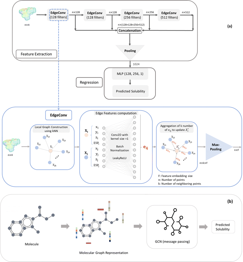
The EdgeConv deep learning model was originally used for the classification and segmentation of 3D objects (x, y, z). In our work we have adapted it for solubility prediction (regression problem) by processing ESP maps (x, y, z, ESP). The feature extraction process involves four EdgeConv operations applied to the raw ESP map using kernels of sizes 128, 128, 256, and 512 (Fig. 1). The outputs of these operations are concatenated to form a matrix of dimensions 3000 × 1024. Subsequently, a combination of average and maximum pooling is applied, resulting in a 1024 array. This output from the feature extraction is then connected to the Multi-Layer Perceptron (MLP) regression component, and both parts' parameters are simultaneously trained to enhance the accuracy of the solubility prediction.
The EdgeConv operation as the building block of model architecture begins by constructing a local neighborhood graph for each point in each point cloud (ESP map). This is achieved by identifying the top k nearest neighbor points, determined by the minimum distance in the feature space of points. Following this, a 2D convolution with a kernel size of 1, coupled with a Leaky ReLU activation function, is utilized to calculate edge features for each pair of points within the graph. Then, these edge features, originating from all edges connected to a vertex, are aggregated using permutation-invariant operators such as maximum and average. This process updates the representation of the vertex. The dynamic nature of EdgeConv adjusts the k nearest neighbors after each layer, ensuring the relevance of local neighbors to the updated features (Fig. 1).
In more detail, the embedding h(k)u, corresponding to each node  , is updated during each iteration of message-passing by aggregating information from the u's graph neighborhood
  . The updating node u at kth message passing iteration can be formulated as follows:
 | (1) |
AGGREGATE is a permutation invariant differentiable function that is responsible for passing embeddings (referred to as the “message”) from a target node's neighbors to the target node. The UPDATE function, on the other hand, updates the nodes' features by incorporating the received information from neighboring nodes as well as their own features at previous step. In our work, we employed four message-passing or graph convolution layers with an embedding size of 128, using weighted summation as the ‘AGGREGATE’ function and ReLU as the ‘UPDATE’ function. Subsequently, global pooling is applied to all nodes' updated features after the last convolutional layer, utilizing both mean and max pooling and concatenating the results into a single vector. This concatenated vector undergoes further processing through a fully connected layer to predict solubility.
We utilized feature importance analysis from the Random Forest algorithm to identify and select approximately the top 20% of extracted features from the ESP map and Mordred descriptors. These features were chosen based on their significance and relevance to solubility prediction. These features were carefully chosen due to their significance and relevance in predicting solubility. In this process, decision trees within the algorithm evaluate each feature's capability to divide data into more consistent subsets, resulting in a reduction of disorder and uncertainty in data classification. Features that contribute to a more significant reduction in the disorder are assigned higher importance scores, emphasizing their influential role in predicting solubility. We reduced the number of tabular features from 1905 to 525 (consisting of 500 features selected from the original 1826 Mordred features, and 25 from ESP) to improve computational efficiency in the model and mitigate overfitting during training.
The extracted and selected features were then fed into an XGBoost model. XGBoost, short for eXtreme Gradient Boosting, stands out as a robust predictive model in machine learning.57 It works by combining predictions from multiple weak learners in a step-by-step manner. The algorithm improves its predictions by minimizing errors identified by the group of learners. This improvement is achieved through optimization of an objective function that considers both a loss term and regularization terms, striking a balance between model complexity and accuracy to prevent overfitting. We used 300 trees as learners in XGBoost with a maximum depth of 3 and a learning rate of 0.1 as the best hyperparameters (after a random search for tuning).
2.4 Data preprocessing
To ensure an unbiased evaluation of the model's generalization performance, we initially split the data randomly into training and test sets with an 80![[thin space (1/6-em)]](https://www.rsc.org/images/entities/char_2009.gif) :
:![[thin space (1/6-em)]](https://www.rsc.org/images/entities/char_2009.gif) 20 ratio. Subsequently, we normalized both train and test data for model training and evaluation, respectively. Normalization of input data is crucial for the effectiveness of machine learning models. Maintaining consistent scales across features prevents certain variables from exerting a disproportionate impact during the training process. In our study, node and edge features in graph data, being one-hot encoded, do not require normalization. However, for the other two modalities, point cloud and tabular features, we employed the Min–Max scaling approach. Specifically, ESP maps, representing point cloud data, underwent careful normalization to preserve the spatial shape of molecules. To achieve this, we ensured consistency in the normalization process by first calculating the global minimum and maximum values across all x, y, and z coordinates in all training data. Min–Max scaling was then applied to each coordinate independently using these global min and max values, preserving the relative spatial relationships of the points in the normalized feature space. The fourth feature of each point in the point clouds, which is independent of the spatial coordinates, was scaled based on the global minimum and maximum ESP values calculated from the entire training dataset. Furthermore, for tabular data, all extracted features were normalized to a uniform range of (0, 1), taking into account the minimum and maximum values of each feature across all entries.
20 ratio. Subsequently, we normalized both train and test data for model training and evaluation, respectively. Normalization of input data is crucial for the effectiveness of machine learning models. Maintaining consistent scales across features prevents certain variables from exerting a disproportionate impact during the training process. In our study, node and edge features in graph data, being one-hot encoded, do not require normalization. However, for the other two modalities, point cloud and tabular features, we employed the Min–Max scaling approach. Specifically, ESP maps, representing point cloud data, underwent careful normalization to preserve the spatial shape of molecules. To achieve this, we ensured consistency in the normalization process by first calculating the global minimum and maximum values across all x, y, and z coordinates in all training data. Min–Max scaling was then applied to each coordinate independently using these global min and max values, preserving the relative spatial relationships of the points in the normalized feature space. The fourth feature of each point in the point clouds, which is independent of the spatial coordinates, was scaled based on the global minimum and maximum ESP values calculated from the entire training dataset. Furthermore, for tabular data, all extracted features were normalized to a uniform range of (0, 1), taking into account the minimum and maximum values of each feature across all entries.
In the results section, the performance of the proposed models will be evaluated using three metrics: Mean Absolute Error (MAE), Root Mean Squared Error (RMSE), and R-squared (R2). These metrics are calculated using the formulae defined in ESI (S2).†
3. Results and discussion
3.1 Datasets analysis
![[thin space (1/6-em)]](https://www.rsc.org/images/entities/char_2009.gif) S), depicted in Fig. 3, ranges from poorly soluble drug molecules (typically with log
S), depicted in Fig. 3, ranges from poorly soluble drug molecules (typically with log![[thin space (1/6-em)]](https://www.rsc.org/images/entities/char_2009.gif) S less than −1.5) to more soluble ones (with log
S less than −1.5) to more soluble ones (with log![[thin space (1/6-em)]](https://www.rsc.org/images/entities/char_2009.gif) S greater than −1.5), with a predominant presence of poorly soluble drugs. This pattern underscores the datasets' emphasis on compounds dealing with poor water solubility, aligning with the goal of identifying drugs susceptible to bioavailability issues.
S greater than −1.5), with a predominant presence of poorly soluble drugs. This pattern underscores the datasets' emphasis on compounds dealing with poor water solubility, aligning with the goal of identifying drugs susceptible to bioavailability issues.
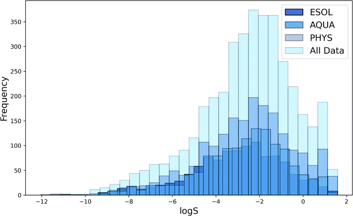 | ||
| Fig. 3 Solubility distribution of molecules in selected datasets of All Data, ESOL, PHYS and AQUA.44 | ||
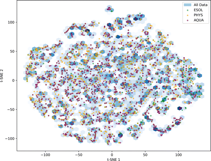 | ||
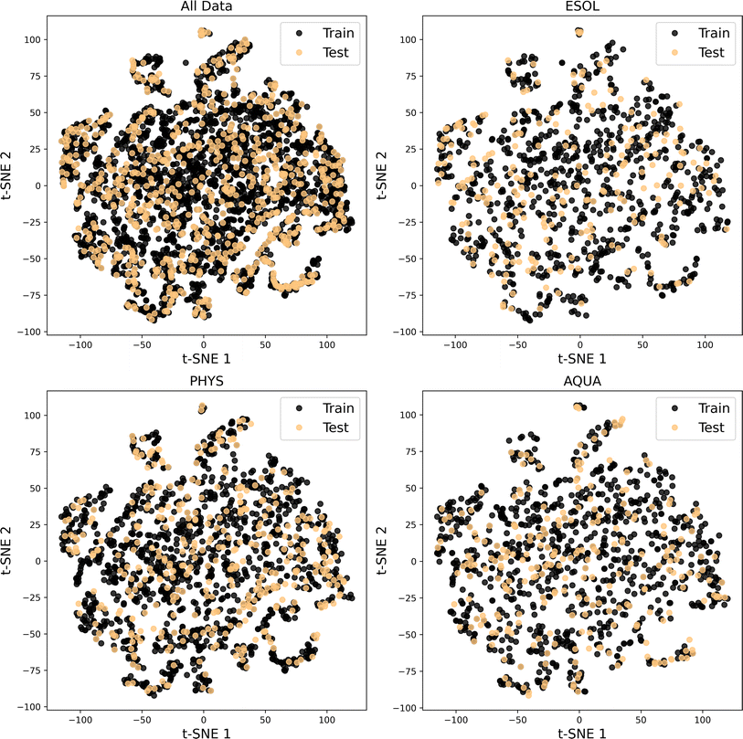
| Fig. 4 t-SNE based analysis of chemical space covered in each dataset of All Data, ESOL, PHYS and AQUA. | ||
For each evaluation, we randomly selected 20% of the molecules in each dataset as unseen or test data for the model. The chemical space distribution in the training and test data is illustrated in Fig. 5, confirming that the test data for the four considered datasets is diverse and capable of validating the trained model across a wide range of chemical space.
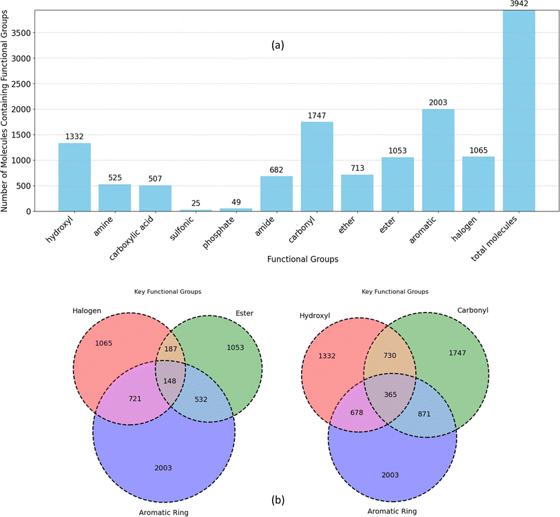 | ||
| Fig. 6 (a) Frequency of functional groups in all unique molecules in datasets, (b) overlap of functional groups and aromatic rings within the molecules. | ||
The Venn diagrams in Fig. 6b delve deeper into the co-occurrence of key functional groups with aromatic rings in datasets molecules. Notably, carbonyl, hydroxyl, and halogen groups exhibit higher overlap with aromatic rings compared to ester. Aromatic rings are significantly more prevalent in conjunction with carbonyl and hydroxyl groups compared to ester and halogen groups (more than twice). Furthermore, the diagram highlights a considerably lower overlap between halogen and ester groups compared to their respective associations with aromatic rings. While both hydroxyl and carbonyl groups frequently coexist with aromatic rings more than with each other. Collectively, this analysis illustrates the diverse chemical space within the dataset, emphasizing the prevalence of specific functional groups and their interactions with aromatic rings.
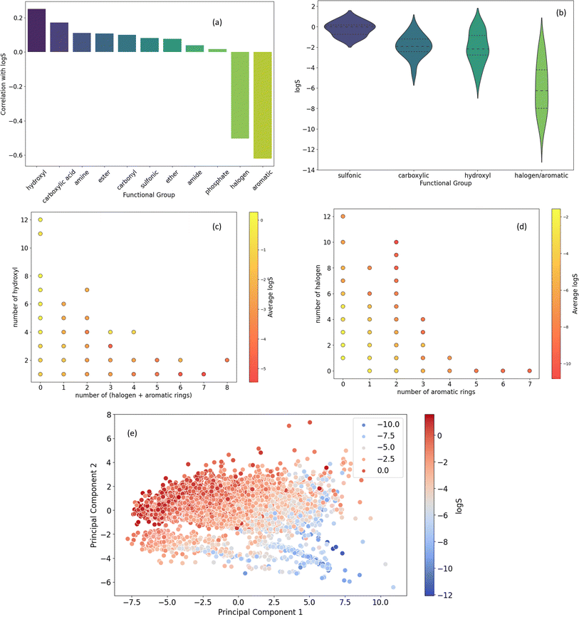
![[thin space (1/6-em)]](https://www.rsc.org/images/entities/char_2009.gif) S. A strong negative correlation is observed between log
S. A strong negative correlation is observed between log![[thin space (1/6-em)]](https://www.rsc.org/images/entities/char_2009.gif) S and the count of halogens and aromatic rings, indicating that the presence of these groups increases hydrophobicity and decreases solubility. Conversely, a positive correlation exists between log
S and the count of halogens and aromatic rings, indicating that the presence of these groups increases hydrophobicity and decreases solubility. Conversely, a positive correlation exists between log![[thin space (1/6-em)]](https://www.rsc.org/images/entities/char_2009.gif) S and the number of hydroxyl and carboxylic acid groups, suggesting their hydrophilic nature. While amine, ester, and carbonyl groups also exhibit positive correlations with log
S and the number of hydroxyl and carboxylic acid groups, suggesting their hydrophilic nature. While amine, ester, and carbonyl groups also exhibit positive correlations with log![[thin space (1/6-em)]](https://www.rsc.org/images/entities/char_2009.gif) S, these relationships are less pronounced.
S, these relationships are less pronounced.
Fig. 7b presents the distribution of log![[thin space (1/6-em)]](https://www.rsc.org/images/entities/char_2009.gif) S values for molecules containing specific functional groups. The presence of sulfonic acid groups is associated with significantly higher solubility compared to other groups. Additionally, the presence of halogen or aromatic rings tends to correlate with a lower solubility range, with a median of −6 (log
S values for molecules containing specific functional groups. The presence of sulfonic acid groups is associated with significantly higher solubility compared to other groups. Additionally, the presence of halogen or aromatic rings tends to correlate with a lower solubility range, with a median of −6 (log![[thin space (1/6-em)]](https://www.rsc.org/images/entities/char_2009.gif) S).
S).
Fig. 7c and d delve deeper into the relationship between functional group counts and average log![[thin space (1/6-em)]](https://www.rsc.org/images/entities/char_2009.gif) S values. Fig. 7c highlights the strong positive correlation between the number of hydroxyl groups and average log
S values. Fig. 7c highlights the strong positive correlation between the number of hydroxyl groups and average log![[thin space (1/6-em)]](https://www.rsc.org/images/entities/char_2009.gif) S, particularly when combined with a lower count of halogen and aromatic rings. Fig. 7d suggests that an increasing number of halogen and aromatic rings generally correlates with a decreasing average solubility.
S, particularly when combined with a lower count of halogen and aromatic rings. Fig. 7d suggests that an increasing number of halogen and aromatic rings generally correlates with a decreasing average solubility.
Fig. 7e employs Principal Component Analysis (PCA) to visualize the relationship between molecular features and solubility. The plot reveals a clear trend where molecules with higher solubility tend to cluster in the upper left quadrant, suggesting that the underlying molecular features in this region are associated with increased hydrophilicity.
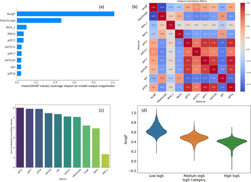
In addition to structural analysis, we also evaluated key features from the ESP map and Mordred descriptors. Fig. 8a ranks the top 10 features by their SHAP values, which will be discussed in the Explainability analysis section (below). A comprehensive list of all Mordred descriptors is available in their original source,59 but descriptions of the top 10 features, including those from ESP maps, are provided in ESI (S3).† Among these, SLogP, a Mordred estimate of lipophilicity, stands out as the most influential descriptor. It is followed by FilteritLogS, a Mordred estimate of solubility, and Beta_1, the strongest hydrogen bond acceptor parameter. Additionally, several piPC descriptors (piPC2, piPC6, piPC7), which are related to π-electron count, also exhibit significant impact.
The high correlations observed among piPC descriptors indicate potential redundancy (Fig. 8b), while Beta_1 stands out with minimal correlation to other features, highlighting its unique contribution and its role in reducing multicollinearity. Fig. 8c visualizes the sum of absolute correlation values for each descriptor, reinforcing Beta_1's low correlation with other features and highlighting the interconnectedness of piPC descriptors. Overall, SLogP and Beta_1 can be identified as key features for solubility prediction in terms of correlation with solubility and minimal redundancy.
Fig. 8d explores the distribution of SLogP across different solubility ranges. The violin plot reveals a clear trend of increasing SLogP with higher solubility categories, underscoring its role as a key determinant of solubility. The solubility ranges are categorized as follows: low log![[thin space (1/6-em)]](https://www.rsc.org/images/entities/char_2009.gif) S (below the 25th percentile), medium log
S (below the 25th percentile), medium log![[thin space (1/6-em)]](https://www.rsc.org/images/entities/char_2009.gif) S (between the 25th and 75th percentiles), and high log
S (between the 25th and 75th percentiles), and high log![[thin space (1/6-em)]](https://www.rsc.org/images/entities/char_2009.gif) S (above the 75th percentile). The distribution of the remaining top 9 features can be found in ESI (S4).†
S (above the 75th percentile). The distribution of the remaining top 9 features can be found in ESI (S4).†
3.2 Models performance on test data
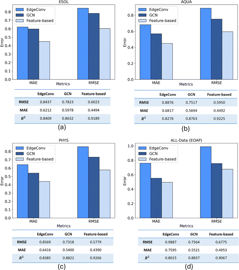
All three proposed models trained individually on 80% of train split of four considered datasets. Then the predictive performances of models on different datasets were quantified using key performance metrics of MAE, RMSE, and R2. Therefore, the prediction results of three models are compared to each other for test split of each dataset of ESOL, AQUA, PHYS, and All Data in Fig. 9. Also, a comparison of three models in terms of number of parameters, training and prediction time are included in ESI (S5).†Each of the three proposed models was trained independently on 80% of the training split across the four datasets under consideration. Subsequently, the predictive performance of the models on various datasets was assessed using key performance metrics, including MAE, RMSE, and R2. The comparison of the prediction results for the three models on the test split of each dataset (ESOL, AQUA, PHYS, and All Data) is depicted in Fig. 9. The findings reveal that, for the ESOL dataset, both the EdgeConv and GCN models exhibit nearly identical performance, while the feature-based model outperforms them. Assessing the results across the other three datasets, a consistent pattern emerges, with the feature-based model consistently achieving the best results, followed by GCN and EdgeConv as the second and third in rank, respectively. The three models exhibited their optimal predictive performance on the PHYS dataset, achieving RMSE scores of 0.856, 0.731, and 0.577 for EdgeConv, GCN, and the feature-based model, respectively.
The RMSE values above 0.5 can largely be attributed to unavoidable measurement errors, as evidenced by the significant variability in solubility data from two well-known solubility challenges (SC-1 and SC-2),60 where standard deviations were 0.6 and 0.17 log units, respectively. Since interlaboratory deviations are often unreported in experimental datasets, similar levels of measurement error are likely, making it challenging to achieve RMSE values significantly below 0.5.
Among the datasets, all models demonstrated their superior prediction performance when trained on PHYS dataset. Unlike the other datasets, where records had variable weights due to inconsistent solubility measurements, all records in PHYS were assigned a weight of 1,31 indicating high consistency and low uncertainty. Training models with the PHYS dataset, therefore, led to the best predictive and generalization performance, reflecting its higher data quality.
An alternative evaluation of model performance for each dataset is illustrated in Fig. 10. The scatter plot showcases the experimental and predicted values of solubility for the test data. A bold line represents a perfect match, while two dashed lines, with a distance equal to the RMSE, provide a visual indication of the quality of the matching between predictions and experimental results. Additionally, a histogram illustrating the distribution of errors accompanies each scatter plot, providing complementary insights into the predictive performance. The convergence of results from three distinct representations mutually reinforces their validity. In a comprehensive comparison across all datasets, the feature-based model consistently exhibits superior predictive outcomes, showcasing excellence in performance metrics, prediction versus experimental matching (nearly 0.918 on average), and error distribution. Notably, this model demonstrates minimal fluctuations across the four datasets, with an average MAE and RMSE of 0.458 and 0.613, respectively. This highlights the significance of an efficient molecular representation, as evidenced by the superior performance of the less complex XGBoost model when fed with features extracted from a molecular mix with ESP maps. This emphasizes the effectiveness of a simple, yet efficient data structure (tabular extracted features) combined with a machine learning technique. It outperforms the more complex end-to-end deep learning methods in mapping unstructured point-cloud-based ESP maps and molecular graphs to solubility.
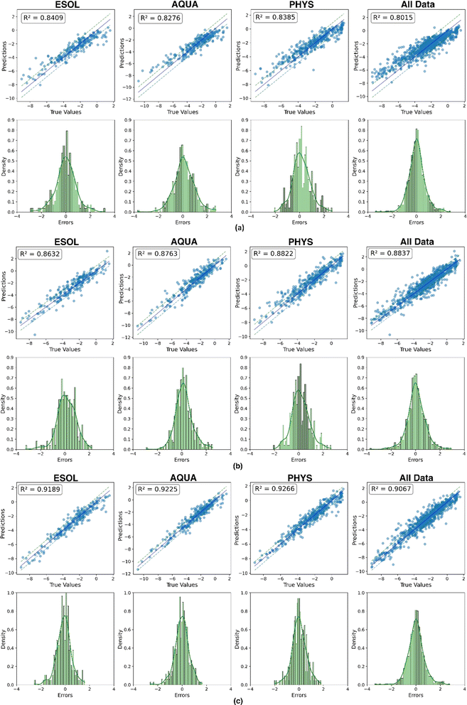 | ||
| Fig. 10 Plot of predicted vs. experimental solubility and histogram distribution of prediction errors across (a) EdgeConv, (b) GCN and (c) feature-based. | ||
In more detail, we believe that the feature-based model outperformed EdgeConv and GCN in predicting solubility due to its comprehensive integration of various molecular features. EdgeConv, which relies solely on ESP maps, excels in capturing charge distribution, polarity, and molecular shape. However, ESP maps often struggle with non-polar and hydrophobic molecules, which show minimal charge separation and result in relatively flat ESP maps. This limitation reduces the effectiveness of ESP maps in extracting meaningful interaction information for these types of molecules.
On the other hand, GCNs analyze atomic connectivity and molecular bonds through atom connectivity graphs. While GCNs effectively map the connectivity and topological structure, they lack direct consideration of electronic properties such as charge distribution and molecular shape. This gap can lead to incomplete predictions, especially when detailed electronic information is crucial for accurate solubility predictions.
The feature-based model combines ESP-derived features with a comprehensive array of Mordred descriptors to overcome the limitations of individual methods. By integrating hydrogen bonding parameters and spatial features from ESP maps with a wide range of Mordred descriptors—covering topological indices, molecular connectivity, complexity, geometric properties, and electronic characteristics—the model offers a detailed and multifaceted representation of molecules. This fusion enhances its capability to accurately predict solubility, particularly for non-polar or hydrophobic molecules where ESP maps alone may be insufficient. As a result, the feature-based model provides a more complete and nuanced view of molecular properties, leading to superior predictive performance.
3.3 Ensemble prediction results
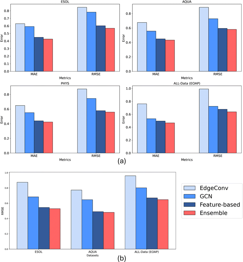
In this section, we present the results of an Ensemble model that combines the predictions of three previously discussed models to enhance overall performance and robustness. The Ensemble model uses a weighted summation approach, where the weights are determined by the inverse of the RMSE values of each individual model (details of formulae are in ESI, S2†). This weighting scheme ensures that models with smaller RMSE values have a greater influence on the final predicted solubility values. Obviously, the complexity and the computational effort increases exponentially.Table 1 summarizes the performance metrics of the Ensemble model, including R2, RMSE, and MAE, across four datasets. Additionally, Fig. 11a illustrates the comparative performance of the Ensemble model with respect to the individual models. The Ensemble model consistently outperforms each individual model in terms of all three metrics across all datasets. This performance improvement is attributed to the Ensemble method's ability to integrate predictions from multiple models, thereby mitigating individual model biases and leveraging their collective strengths. By incorporating predictions from three distinct models, each based on different molecular representations, the Ensemble model offers increased confidence in its predictions. A complete comparison summary of models, where small scale ML models based on all Mordred features is included in the ESI (S6).† Moreover, the mean error distribution based on specific functional groups is also included in the ESI (S7).†
| Model | ESOL | AQUA | PHYS | ALL-data (EOAP) | ||||||||
|---|---|---|---|---|---|---|---|---|---|---|---|---|
| RMSE | MAE | R 2 | RMSE | MAE | R 2 | RMSE | MAE | R 2 | RMSE | MAE | R 2 | |
| Ensemble | 0.569 | 0.425 | 0.928 | 0.580 | 0.432 | 0.926 | 0.559 | 0.423 | 0.931 | 0.638 | 0.466 | 0.917 |
3.4 Transferability study results
The transferability of the four models, including the Ensemble model, was evaluated by training on the highest quality dataset (PHYS) and testing on three additional datasets: ESOL, AQUA, and All-Data. The results are presented in Fig. 11b and Table 2 which display the RMSE, MAE, and R2 values for each model and the Ensemble across these test datasets. The transferability analysis highlights the generalization capabilities of all models as they indicated roughly the same level of performance compared to their results based on only 20% test data. The feature-based and Ensemble models demonstrated generally superior performance compared to the individual models, indicating its robustness and effectiveness in making accurate predictions across diverse datasets.| Models | ESOL | AQUA | All-Data (EOAP) | ||||||
|---|---|---|---|---|---|---|---|---|---|
| RMSE | MAE | R 2 | RMSE | MAE | R 2 | RMSE | MAE | R 2 | |
| EdgeConv | 0.874 | 0.645 | 0.835 | 0.887 | 0.586 | 0.827 | 0.959 | 0.722 | 0.815 |
| GCN | 0.683 | 0.492 | 0.899 | 0.752 | 0.464 | 0.876 | 0.802 | 0.567 | 0.871 |
| Feature-based | 0.545 | 0.365 | 0.935 | 0.595 | 0.338 | 0.922 | 0.670 | 0.455 | 0.910 |
| Ensemble | 0.529 | 0.373 | 0.940 | 0.481 | 0.341 | 0.947 | 0.647 | 0.456 | 0.916 |
3.5 Results on solubility challenge dataset
To evaluate the accuracy and generalizability of our Ensemble model relative to previous predictive works, we utilized the Solubility Challenge 2019 dataset, also known as the second solubility challenge (SC-2). This experimental intrinsic solubility dataset is particularly valuable for comparison as it demonstrates improved interlaboratory reproducibility, with a standard deviation of 0.17 log units, compared to the 0.6 log units reported in the first solubility challenge (SC-1).The SC-2 dataset comprises intrinsic solubility measurements of 100 druglike compounds, curated from multiple published sources. For our evaluation, we performed DFT calculations and prepared input data for our models. Importantly, we excluded all 100 molecules from our selected training dataset (PHYS) to meet the challenge's requirements. After training our models, we used the Ensemble model to assess its performance. The evaluation metrics of RMSE and MAE for our Ensemble model are 0.865 and 0.670, respectively.
In a comparative study by Llinas et al.,60 37 predictive approaches were compared on the SC-2 dataset, utilizing diverse training data, models (spanning from Multi-Linear Regression to advanced methods like LightGBM, ANN, and GCN), and molecular representations (encompassing RDKit descriptors, Morgan fingerprints, and graph-based representations). Reported RMSE values for these 37 models ranged from 1.06 to 3.00, with an average of 1.62. Notably, our Ensemble model outperformed all these methods, achieving a lower RMSE. Our predictions for SC2 molecules, including compound names, SMILES, and mean experimental solubility, are detailed in the second sheet of the ESIData excel file.†
3.6 Explainability analysis
In this section, we perform an explainability analysis on our feature-based model, which is the best among the three evaluated models. To achieve this, we use the SHAP61 (SHapley Additive exPlanations) method to enhance the interpretability and transparency of our ML-based model's predictions. The SHAP approach is based on Shapley values, which are rooted in cooperative game theory and are used to distribute a total gain among players based on their individual contributions.In the context of feature-based ML models, Shapley values indicate how each input feature contributes to the deviation of a particular prediction from the average prediction. This method is additive, meaning the sum of all features' SHAP values equals the difference between the model's prediction for a specific instance and the average prediction across all instances. This explainability analysis helps build trust in the model's decisions, thereby improving transparency and interpretability.
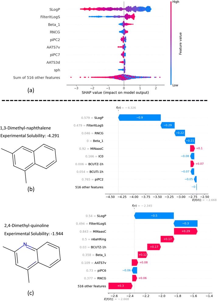
In Fig. 12a, the beeswarm plot illustrates the overall effect of the top 10 features on the model's predictions using SHAP values. This plot shows how different levels of features influence the model's output. Negative SHAP values on the x-axis indicate a negative impact of the feature on predicted solubility, while positive values indicate a positive effect. The color bar corresponds to low (blue) and high (red) feature values and the range in between.
From Fig. 12a, we can interpret that higher SLogP values lead to a more negative impact on solubility, and vice versa. In contrast, the trends for FilterItLogS and Beta_1 show a consistent effect on predicted solubility, which aligns with chemical intuition. For instance, higher Beta_1 values indicate a stronger hydrogen bond acceptor in molecules, resulting in higher solubility. Additionally, the plot suggests that low sphericity (sph) negatively impacts molecule solubility, whereas high sphericity has a negligible effect.
The SHAP waterfall plots in Fig. 12b and c illustrate the application of our feature-based model to 1,3-dimethyl-naphthalene and 2,4-dimethyl-quinoline, respectively. These molecules were selected to assess the impact of replacing a methine group with a nitrogen atom to form a pyridine ring on the molecular properties predicted by the model. The y-axis in each plot shows the normalized feature values on a scale from 0 to 1. The mean prediction of the model across all data is displayed at the bottom of the figures (E[f(x)]), while the predicted solubility for each molecule is shown at the top (f(x)).
The SHAP values, represented by blue and red bars, indicate the contribution of each feature to the specific solubility prediction relative to the average predicted solubility. SLogP, as the most influential feature, affects solubility by −0.9 and −0.5 for the first and second molecules, respectively. Comparing the contributions of features for the two examples, we observe that with the addition of a pyridine ring, Beta_1 increases significantly from 0 to 0.358 (on a scale of 0 to 1), resulting in a 0.33 increase in average predicted solubility. Similarly, an increase of 0.331 in RNCG, which represents the relative negative charge, contributes to a net increase of 0.28 in solubility. Further explanation analysis of four additional examples of molecule pairs is provided in Fig. S4 and S5 in ESI (S8).†
4. Conclusions
This study presented three machine learning-based models for the prediction of solubility of pharmaceuticals in aqueous medium at 25 °C. Each model employs distinct molecular representation modalities. The initial two approaches leveraged end-to-end deep learning, utilizing ESP maps and molecular graphs. In contrast, the third approach employed a simpler XGBoost model, incorporating features extracted from ESP maps and Mordred descriptors, focusing on the most crucial molecular properties for aqueous solubility prediction. High-quality and curated datasets were employed for model training, and their diversity was carefully assessed to gain insights into the generalizability of the developed models across a broad spectrum of molecules. The t-SNE analysis revealed that while all three high-quality datasets demonstrated appealing diversity, AQUA and PHYS datasets exhibited superior diversity and sparsity compared to ESOL.Through the comprehensive comparison of three methodologies, it becomes evident that the combined utilization of ESP map features and Mordred descriptors, yielding an average RMSE of 0.613, outshines the performance of more intricate deep learning models such as EdgeConv (0.893) and GCN (0.755). This underscores a crucial takeaway: the effectiveness of the input data representation holds greater significance than the complexity of the model. An ensemble of the three models improved the error metrics for all datasets. The Ensemble model achieved an RMSE of 0.865 on the Solubility Challenge 2019, surpassing the average RMSE of 1.62 reported by 37 models. Transferability analysis confirmed the robustness of both the individual models and their ensemble across datasets. The explainability analysis demonstrated the interpretability of key features in solubility predictions.
Data availability
A repository containing the data and associated analysis code has been made available on GitHub (https://github.com/amingh1995/Aqueous-Solubility-Prediction).Author contributions
M. A. Ghanavati: conceptualization, data curation, formal analysis, methodology, visualization, writing – original draft; S. Ahmadi: conceptualization, data curation, writing – review & editing; S. Rohani: conceptualization, methodology, writing – review & editing, supervision.Conflicts of interest
There are no conflicts to declare.Acknowledgements
The authors acknowledge the Natural Sciences and Engineering Research Council of Canada (NSERC) for financial support. This research was enabled in part by support provided by Compute Canada (https://www.computecanada.ca) for computation and granting access to Gaussian software and GPU-based training of deep learning models.References
- D. Singh, N. Bedi and A. K. Tiwary, Enhancing Solubility of Poorly Aqueous Soluble Drugs: Critical Appraisal of Techniques, J. Pharm. Invest., 2018, 48(5), 509–526, DOI:10.1007/s40005-017-0357-1.
- C. Fink, D. Sun, K. Wagner, M. Schneider, H. Bauer, H. Dolgos, K. Mäder and S.-A. Peters, Evaluating the Role of Solubility in Oral Absorption of Poorly Water-Soluble Drugs Using Physiologically-Based Pharmacokinetic Modeling, Clin. Pharmacol. Ther., 2020, 107(3), 650–661, DOI:10.1002/cpt.1672.
- Y. A. Abramov, G. Sun, Q. Zeng, Q. Zeng and M. Yang, Guiding Lead Optimization for Solubility Improvement with Physics-Based Modeling, Mol. Pharm., 2020, 17(2), 666–673, DOI:10.1021/acs.molpharmaceut.9b01138.
- Y. Kawabata, K. Wada, M. Nakatani, S. Yamada and S. Onoue, Formulation Design for Poorly Water-Soluble Drugs Based on Biopharmaceutics Classification System: Basic Approaches and Practical Applications, Int. J. Pharm., 2011, 420(1), 1–10, DOI:10.1016/j.ijpharm.2011.08.032.
- D. V. Bhalani, B. Nutan, A. Kumar and A. K. Singh Chandel, Bioavailability Enhancement Techniques for Poorly Aqueous Soluble Drugs and Therapeutics, Biomedicines, 2022, 10(9), 2055 CrossRef CAS.
- A. Charalabidis, M. Sfouni, C. Bergström and P. Macheras, The Biopharmaceutics Classification System (BCS) and the Biopharmaceutics Drug Disposition Classification System (BDDCS): Beyond Guidelines, Int. J. Pharm., 2019, 566, 264–281, DOI:10.1016/j.ijpharm.2019.05.041.
- J. A. Barrett, W. Yang, S. M. Skolnik, L. M. Belliveau and K. M. Patros, Discovery Solubility Measurement and Assessment of Small Molecules with Drug Development in Mind, Drug Discovery Today, 2022, 27(5), 1315–1325, DOI:10.1016/j.drudis.2022.01.017.
- Y. Ran and S. H. Yalkowsky, Prediction of Drug Solubility by the General Solubility Equation (GSE), J. Chem. Inf. Comput. Sci., 2001, 41(2), 354–357 CrossRef CAS.
- A. Fredenslund, R. L. Jones and J. M. Prausnitz, Group-contribution Estimation of Activity Coefficients in Nonideal Liquid Mixtures, AIChE J., 1975, 21(6), 1086–1099 CrossRef CAS.
- G. Maurer and J. M. Prausnitz, On the Derivation and Extension of the UNIQUAC Equation, Fluid Phase Equilib., 1978, 2(2), 91–99 CrossRef CAS.
- W. G. Chapman, K. E. Gubbins, G. Jackson and M. Radosz, SAFT: Equation-of-State Solution Model for Associating Fluids, Fluid Phase Equilib., 1989, 52, 31–38, DOI:10.1016/0378-3812(89)80308-5.
- F. Eckert and A. Klamt, Fast Solvent Screening via Quantum Chemistry: COSMO-RS Approach, AIChE J., 2002, 48(2), 369–385 CrossRef CAS.
- M. Kuentz and C. A. S. Bergström, Synergistic Computational Modeling Approaches as Team Players in the Game of Solubility Predictions, J. Pharm. Sci., 2021, 110(1), 22–34 CrossRef CAS.
- F. Silva, F. Veiga, S. P. J. Rodrigues, C. Cardoso and A. C. Paiva-Santos, COSMO Models for the Pharmaceutical Development of Parenteral Drug Formulations, Eur. J. Pharm. Biopharm., 2023, 187, 156–165, DOI:10.1016/j.ejpb.2023.04.019.
- K. Lüder, L. Lindfors, J. Westergren, S. Nordholm and R. Kjellander, In Silico Prediction of Drug Solubility. 3. Free Energy of Solvation in Pure Amorphous Matter, J. Phys. Chem. B, 2007, 111(25), 7303–7311 CrossRef.
- Z. Bjelobrk, D. Mendels, T. Karmakar, M. Parrinello and M. Mazzotti, Solubility Prediction of Organic Molecules with Molecular Dynamics Simulations, Cryst. Growth Des., 2021, 21(9), 5198–5205 CrossRef CAS.
- A. Klamt, F. Eckert, M. Hornig, M. E. Beck and T. Bürger, Prediction of Aqueous Solubility of Drugs and Pesticides with COSMO-RS, J. Comput. Chem., 2002, 23(2), 275–281 CrossRef CAS PubMed.
- A. Klamt, Conductor-like Screening Model for Real Solvents: A New Approach to the Quantitative Calculation of Solvation Phenomena, J. Phys. Chem., 1995, 99(7), 2224–2235 CrossRef CAS.
- J. R. Espinosa, J. M. Young, H. Jiang, D. Gupta, C. Vega, E. Sanz, P. G. Debenedetti and A. Z. Panagiotopoulos, On the Calculation of Solubilities via Direct Coexistence Simulations: Investigation of NaCl Aqueous Solutions and Lennard-Jones Binary Mixtures, J. Chem. Phys., 2016, 145(15), 154111, DOI:10.1063/1.4964725.
- A. L. Benavides, J. L. Aragones and C. Vega, Consensus on the Solubility of NaCl in Water from Computer Simulations Using the Chemical Potential Route, J. Chem. Phys., 2016, 144(12), 124504, DOI:10.1063/1.4943780.
- S. Boothroyd, A. Kerridge, A. Broo, D. Buttar and J. Anwar, Solubility Prediction from First Principles: A Density of States Approach, Phys. Chem. Chem. Phys., 2018, 20(32), 20981–20987, 10.1039/C8CP01786G.
- K. T. Butler, D. W. Davies, H. Cartwright, O. Isayev and A. Walsh, Machine Learning for Molecular and Materials Science, Nature, 2018, 559(7715), 547–555, DOI:10.1038/s41586-018-0337-2.
- D. Morgan and R. Jacobs, Opportunities and Challenges for Machine Learning in Materials Science, Annu. Rev. Mater. Res., 2020, 50, 71–103 CrossRef CAS.
- J. C. Dearden, In Silico Prediction of Aqueous Solubility, Expert Opin. Drug Discovery, 2006, 1(1), 31–52 CrossRef CAS.
- R. B. Hermann, Theory of Hydrophobic Bonding. II. Correlation of Hydrocarbon Solubility in Water with Solvent Cavity Surface Area, J. Phys. Chem., 1972, 76(19), 2754–2759 CrossRef CAS.
- M. C. Sorkun, J. M. V. A. Koelman and S. Er, Pushing the Limits of Solubility Prediction via Quality-Oriented Data Selection, iScience, 2021, 24(1), 101961, DOI:10.1016/j.isci.2020.101961.
- P. Hu, Z. Jiao, Z. Zhang and Q. Wang, Development of Solubility Prediction Models with Ensemble Learning, Ind. Eng. Chem. Res., 2021, 60(30), 11627–11635, DOI:10.1021/acs.iecr.1c02142.
- S. Lee, M. Lee, K.-W. Gyak, S. D. Kim, M.-J. Kim and K. Min, Novel Solubility Prediction Models: Molecular Fingerprints and Physicochemical Features vs. Graph Convolutional Neural Networks, ACS Omega, 2022, 7(14), 12268–12277, DOI:10.1021/acsomega.2c00697.
- Z. Ye and D. Ouyang, Prediction of Small-Molecule Compound Solubility in Organic Solvents by Machine Learning Algorithms, J. Cheminf., 2021, 13(1), 98, DOI:10.1186/s13321-021-00575-3.
- A. D. Vassileiou, M. N. Robertson, B. G. Wareham, M. Soundaranathan, S. Ottoboni, A. J. Florence, T. Hartwig and B. F. Johnston, A Unified ML Framework for Solubility Prediction across Organic Solvents, Digital Discovery, 2023, 2(2), 356–367, 10.1039/D2DD00024E.
- M. Lovrić, K. Pavlović, P. Žuvela, A. Spataru, B. Lučić, R. Kern and M. W. Wong, Machine Learning in Prediction of Intrinsic Aqueous Solubility of Drug-like Compounds: Generalization, Complexity, or Predictive Ability?, J. Chemom., 2021, 35(7–8), e3349 CrossRef.
- J. Wang, Z. Song, L. Chen, T. Xu, L. Deng and Z. Qi, Prediction of CO2 Solubility in Deep Eutectic Solvents Using Random Forest Model Based on COSMO-RS-Derived Descriptors, Green Chem. Eng., 2021, 2(4), 431–440, DOI:10.1016/j.gce.2021.08.002.
- Q. Cui, S. Lu, B. Ni, X. Zeng, Y. Tan, Y. D. Chen and H. Zhao, Improved Prediction of Aqueous Solubility of Novel Compounds by Going Deeper with Deep Learning, Front. Oncol., 2020, 10, 121 CrossRef.
- G. Panapitiya, M. Girard, A. Hollas, J. Sepulveda, V. Murugesan, W. Wang and E. Saldanha, Evaluation of Deep Learning Architectures for Aqueous Solubility Prediction, ACS Omega, 2022, 7(18), 15695–15710 CrossRef CAS.
- P. G. Francoeur and D. R. Koes, SolTranNet–A Machine Learning Tool for Fast Aqueous Solubility Prediction, J. Chem. Inf. Model., 2021, 61(6), 2530–2536, DOI:10.1021/acs.jcim.1c00331.
- Z. Xiong, D. Wang, X. Liu, F. Zhong, X. Wan, X. Li, Z. Li, X. Luo, K. Chen, H. Jiang and M. Zheng, Pushing the Boundaries of Molecular Representation for Drug Discovery with the Graph Attention Mechanism, J. Med. Chem., 2020, 63(16), 8749–8760, DOI:10.1021/acs.jmedchem.9b00959.
- W. Ahmad, H. Tayara and K. T. Chong, Attention-Based Graph Neural Network for Molecular Solubility Prediction, ACS Omega, 2023, 8(3), 3236–3244, DOI:10.1021/acsomega.2c06702.
- S. Lee, H. Park, C. Choi, W. Kim, K. K. Kim, Y.-K. Han, J. Kang, C.-J. Kang and Y. Son, Multi-Order Graph Attention Network for Water Solubility Prediction and Interpretation, Sci. Rep., 2023, 13(1), 957, DOI:10.1038/s41598-022-25701-5.
- O. Wieder, M. Kuenemann, M. Wieder, T. Seidel, C. Meyer, S. D. Bryant and T. Langer, Improved Lipophilicity and Aqueous Solubility Prediction with Composite Graph Neural Networks, Molecules, 2021, 26(20), 6185 CrossRef CAS.
- W. Ahmad, H. Tayara, H. Shim and K. T. Chong, SolPredictor: Predicting Solubility with Residual Gated Graph Neural Network, Int. J. Mol. Sci., 2024, 25(2), 715 CrossRef.
- M. Salahinejad, T. C. Le and D. A. Winkler, Aqueous Solubility Prediction: Do Crystal Lattice Interactions Help?, Mol. Pharm., 2013, 10(7), 2757–2766, DOI:10.1021/mp4001958.
- Y. Ma, Z. Gao, P. Shi, M. Chen, S. Wu, C. Yang, J. Wang, J. Cheng and J. Gong, Machine Learning-Based Solubility Prediction and Methodology Evaluation of Active Pharmaceutical Ingredients in Industrial Crystallization, Front. Chem. Sci. Eng., 2022, 1–13 Search PubMed.
- S. Ahmadi, M. A. Ghanavati and S. Rohani, Machine Learning-Guided Prediction of Cocrystals Using Point Cloud-Based Molecular Representation, Chem. Mater., 2024, 36(3), 1153–1161, DOI:10.1021/acs.chemmater.3c01437.
- J. Meng, P. Chen, M. Wahib, M. Yang, L. Zheng, Y. Wei, S. Feng and W. Liu, Boosting the Predictive Performance with Aqueous Solubility Dataset Curation, Sci. Data, 2022, 9(1), 71, DOI:10.1038/s41597-022-01154-3.
- A. Habib, C. Karmakar and J. Yearwood, Impact of ECG Dataset Diversity on Generalization of CNN Model for Detecting QRS Complex, IEEE Access, 2019, 7, 93275–93285, DOI:10.1109/ACCESS.2019.2927726.
- G. Landrum, RDKit: open-source cheminformatics, http://www.rdkit.org, accessed: 29 Feb 2024 Search PubMed.
- M. J. Frisch, G. W. Trucks, H. B. Schlegel, G. E. Scuseria, Ma. Robb, J. R. Cheeseman, G. Scalmani, V. Barone, G. A. Petersson and H. Nakatsuji, Gaussian 16, Revision A. 03, Gaussian. Inc., Wallingford CT, 2016, vol. 3 Search PubMed.
- A. V. Marenich, C. J. Cramer and D. G. Truhlar, Universal Solvation Model Based on Solute Electron Density and on a Continuum Model of the Solvent Defined by the Bulk Dielectric Constant and Atomic Surface Tensions, J. Phys. Chem. B, 2009, 113(18), 6378–6396, DOI:10.1021/jp810292n.
- S. Grimme, A. Hansen, J. G. Brandenburg and C. Bannwarth, Dispersion-Corrected Mean-Field Electronic Structure Methods, Chem. Rev., 2016, 116(9), 5105–5154, DOI:10.1021/acs.chemrev.5b00533.
- B. Ramsundar, Deepchem.Io, 2016, https://github.com/deepchem/deepchem, accessed: 29 Feb 2024 Search PubMed.
- S. Kearnes, K. McCloskey, M. Berndl, V. Pande and P. Riley, Molecular Graph Convolutions: Moving beyond Fingerprints, J. Comput.-Aided Mol. Des., 2016, 30, 595–608 CrossRef CAS.
- H. Moriwaki, Y.-S. Tian, N. Kawashita and T. Takagi, Mordred: A Molecular Descriptor Calculator, J. Cheminf., 2018, 10(1), 1–14 Search PubMed.
- Y. Wang, Y. Sun, Z. Liu, S. E. Sarma, M. M. Bronstein and J. M. Solomon, Dynamic Graph Cnn for Learning on Point Clouds, ACM Trans. Graphics, 2019, 38(5), 1–12 CrossRef.
- C. R. Qi, H. Su, K. Mo and L. J. Guibas, Pointnet: Deep Learning on Point Sets for 3d Classification and Segmentation, in Proceedings of the IEEE conference on computer vision and pattern recognition, 2017, pp 652–660 Search PubMed.
- C. R. Qi, L. Yi, H. Su and L. J. Guibas, Pointnet++: Deep Hierarchical Feature Learning on Point Sets in a Metric Space, Adv. Neural Inf. Process. Syst., 2017, 30, 5099–5108 Search PubMed.
- W. L. Hamilton, Graph Representation Learning, Morgan & Claypool Publishers, 2020 Search PubMed.
- T. Chen and C. Guestrin, Xgboost: A Scalable Tree Boosting System, in Proceedings of the 22nd acm sigkdd international conference on knowledge discovery and data mining, 2016, pp. 785–794 Search PubMed.
- L. Van der Maaten and G. Hinton, Visualizing Data Using T-SNE, J. Mach. Learn. Res., 2008, 9(11) Search PubMed.
- Mordred Documentation, Mordred Descriptors, https://mordred-descriptor.github.io/documentation/master/descriptors.html. accessed 30 July 2024 Search PubMed.
- A. Llinas, I. Oprisiu and A. Avdeef, Findings of the Second Challenge to Predict Aqueous Solubility, J. Chem. Inf. Model., 2020, 60(10), 4791–4803, DOI:10.1021/acs.jcim.0c00701.
- S. M. Lundberg, S.-I. Lee, A Unified Approach to Interpreting Model Predictions, Proceedings of the 31st International Conference on Neural Information Processing Systems, 2017, pp. 4768–4777 Search PubMed.
Footnote |
| † Electronic supplementary information (ESI) available. See DOI: https://doi.org/10.1039/d4dd00065j |
| This journal is © The Royal Society of Chemistry 2024 |

