Modelling kinetic isotope effects for Swern oxidation using DFT-based transition state theory

Abstract

We investigate the model reported by Giagou and Meyer in 2010 for comparing deuterium kinetic isotope effects (KIEs) computed using density functional theory (DFT) for the intramolecular hydrogen transfer step in the mechanism of the Swern oxidation of alcohols to aldehydes, with those measured by experiment. Whereas the replication of the original computed values for the gas-phase reaction proved entirely successful, several issues were discovered when a continuum solvent model was used. These included uncertainty regarding the parameters and methods used for the calculations and also the coordinates for the original reactant and transition structures, via their provision as data in the ESI. The original conclusions, in which a numerical mis-match between the magnitude of the computed and experimentally measured KIE was attributed to significant deviations from transition structure theory, are here instead rationalised as a manifestation of basis-set effects in the computation. Transition state theory appears to be operating successfully. We now recommend the use of basis sets of triple- or quadruple-ζ quality, rather than the split-valence level previously employed, that dispersion energy corrections be included and that a continuum solvent model using smoothed reaction cavities is essential for effective geometry optimisation and hence accurate normal coordinate analysis. An outlying experimental KIE obtained for chloroform as solvent is attributed to a small level of an explicit hydrogen bonded interaction with the substrate. A temperature outlier for the measured KIE at 195 K is suggested for further experimental investigation, although it may also be an indication of an unusually abrupt incursion of hydrogen tunnelling which would need non-Born–Oppenheimer methods in which nuclear quantum effects are included to be more accurately modelled. We predict KIEs for new substituents, of which those for R = NMe₂ are significantly larger than those for R = H. This approach could be useful in designing variations of the Swern reagent that could lead to synthesis of aldehydes incorporating much higher levels of deuterium. The use of FAIR data rather than the traditional model of its inclusion in the ESI is discussed, and two data discovery tools exploiting these FAIR attributes are suggested.

---

1. Introduction

Recently, several reports have documented the oxidation of monodeuterated alcohols to deuterated-enriched aldehydes at synthetically useful levels (85–98 atom% D) by exploitation of a kinetic isotope effect (KIE).^1–4 These methods provide a convenient alternative to pre-existing syntheses of C₁-deuterated alcohols^5,6 since they allow the use of the relatively inexpensive NaBD₄ to install one deuterium atom by reaction with an aldehyde, followed by reoxidation using standard oxidation reagents. The oxidation reagents reported to be successful so far for this latter process are pyridinium chlorochromate-silica,¹ manganese dioxide² and pyridinium chlorochromate.^3,4 Swern oxidation^7,8 that is a sigmatropic pericyclic reaction has also been examined by Giagou and Meyer in 2010 in a comprehensive experimental and computational analysis of this aspect,⁹ finding a relatively low KIE of <3 which would limit the level of deuterium enrichment. We decided therefore to explore the mechanism of this latter reaction computationally, to see if suitable substituents might be capable of increasing the isotope effect and, hence, the level of deuterium enrichment.¹⁰ The combination of experimental and theoretical results had led Giagou and Meyer to conclude that the system may exhibit significant deviations from transition structure theory,⁹ which if correct would mean using a level of computational modelling which goes beyond such theory to ensure that the models correctly predict isotope effects for new variations of the Swern reaction bearing as yet unstudied substituents.

2 Computational methodology

Our approach involved three stages. The first was to attempt to replicate the computational results obtained in 2010 for the reaction shown in Scheme 1 (R = H) and then to explore if changes to the original methodology used could address the apparent issue manifesting as a reported mismatch between the originally measured KIE and their calculated values and attributed to deviation from transition structure theory. Finally, if a robust model for calculating kinetic isotope effects could be identified, it would be used to predict the effects of using new substituents R (Scheme 1). All calculations were performed using Gaussian 16,¹¹ Revisions C.01 or C.02, along with the associated Gaussview program V 6.1.1 (ref. 12) used for input data preparation and output visualisation. Rather than preparing the ESI in the traditional format of a single paginated PDF file used for specifying the coordinates and energies in the original article,⁹ we here adopt the FAIR (Findable, Accessible, Interoperable and Reusable) data principles and metadata protocol¹³ to allow facile replication and re-use of the data generated as part of this work.^14–16 This allows e.g. individual calculations to be identified and cited using a persistent identifier (in the form of a DOI). The datasets associated with this identifier include the original input file complete with all keywords used, a checkpoint file including a full inter-operable wavefunction,¹⁷ a summary log file for easy inspection of the results and elevation of selected properties into globally registered metadata. These are all identified as components of a hierarchical repository data collection. To facilitate the management of these data and the automated preparation of their associated metadata, we used a computational electronic notebook (CHAMP)¹⁸ coupled to a FAIR data¹⁵ research data repository.¹⁴

Scheme 1 R = H; X = D, base = trimethylamine.

3 Results and discussion

3.1 Replication of energies

The starting point for attempting a replication involves two aspects; acquiring the original coordinates for the systems as reported in the ESI for the article⁹ and identifying the appropriate parametric configuration of the software package originally used. The ESI for the computational results – then and indeed often now – took the form of lists of cartesian coordinates computed for the molecules of interest and various energies, including thermodynamically corrected values. Not included in this information – again still a common omission nowadays – were the keywords used to drive the calculations. Some parameters were described in the article text, such as the density functional method employed (B3LYP in this instance), the 6-31+G(d,p) basis set used and the solvation algorithm invoked (IEFPCM), or appearing in the general information at the head of the ESI for the calculations. Other operational parameters such as convergence thresholds for the self-consistent-field and the two-electron integral accuracies would have been set as internal defaults for the program used (Gaussian 03 or G03), although they could have been provided as keywords. Fortunately, the design and evolution of the Gaussian program allow the user to define the original default values for those parameters where they have changed in subsequent program versions, currently Gaussian 16 (or G16). Thus the constants = 1998 keyword resets the fundamental constants to the values used in 2010, the keyword integral = (FineGrid, Acc2E = 10) sets the integral accuracy to the original value and the keyword scrf = (read, iefpcm, solvent = dichloromethane, G03Defaults) resets to the solvation model used in G03. One further inference was made by us about the originally used program keywords in regard to the method used to calculate the normal mode frequencies by computing a second derivative force constant (Hessian) matrix. No analytical second derivatives for this procedure were implemented using G03 and so we infer that the keyword freq(numer) must have been used to generate these values, using a finite difference algorithm.

We set out to compute the total energy via normal mode wavenumbers and the derived Gibbs energy at the coordinates specified in the ESI. These coordinates for the endo-TS series for all the gas-phase and continuum solvent models in the ESI were found to be identical, as were the coordinates for the endo-ylide reactant 2 preceding the transition structure. One possible inference is that gas-phase coordinates were used without re-optimisation for all the solvent models. The coordinates for the exo-TS series were however all different for the solvent/gas phase models, whilst those for reactants 3 were all numerically identical. This leaves open the possibility that the differing coordinates for the exo-TS series had indeed been re-optimised for the continuum solvent and that the inclusion of identical coordinates for the endo-TS series is simply an error resulting from copy/paste operations used to prepare the ESI. We have used an automatic workflow in the CHAMP¹⁸ ELN to publish the original program outputs to a data repository, involving no reformatting or processing of the data files, which are stored intact to eliminate the possibility of such errors.

The difference in total energies as reported in the ESI⁹ for gas phase endo-TS/exo-TS and both 2 and 3 and the present work¹⁹ at the reported coordinates are typically ∼0.000005 kcal mol⁻¹, which can be considered an effective replication. The RMS gradient norms re-computed at the geometries are also <10⁻⁵ au, typical of acceptable convergence values for geometry optimisation, but more particularly a level of accuracy essential for accurate evaluation of vibrational wavenumbers and hence kinetic isotope effects.

A different picture emerges for continuum solvent models. At the geometry for the endo-TS included in the ESI⁹ with dichloromethane indicated as solvent, the total energy quoted as −823.545644624 hartree (all values quoted from ref. 9) was here replicated²⁰ using G16 in G03 mode as −823.545644658 hartree, an accuracy typical for quantum mechanical codes and indeed a testament to the ability of ever-changing computer hardware over the period 2010–2023 to accurately reproduce algorithm-based calculations. The original reported value of ΔG obtained by computing thermal corrections to this energy using the values of the calculated vibrational normal modes was quoted as −823.400723 hartree; no temperature was indicated but is assumed to be ΔG_298.15. The replication value²⁰ is −823.400161 hartree, a difference of ΔΔG_298.15 = 0.35 kcal mol⁻¹. Of more concern was that the gradient norm re-computed under G03 conditions using the quoted ESI coordinates⁹ had a root-mean-square (RMS) value of 0.001477267 au, a value >100-fold larger than the threshold noted above for which the values of the atomic coordinates are considered to be converged. The original value for the gradient norm was not reported, nor were any convergence options that might have been used as keywords for transition structure location. The value of the transition structure imaginary mode at the reported geometry emerges as 364.18i cm⁻¹ for a dichloromethane model²⁰ and 390.0i for the gas-phase,²¹ compared with values of 286i (Table 2 of ref. 9) and 390i cm⁻¹ (Table 1 of ref. 9) respectively, good replication for the latter but less so for the former.

Locating a transition structure is best achieved using a calculated force constant matrix at the initial geometry, which as noted above requires numerical calculation for the G03 code. The modern keyword used in G16 for such a location is opt(calcfc, ts), but this presumes that analytic force constants are available. We decided to see whether, using only G03 options, the gradient norm could be reduced below 0.001477267 au by adopting the following method. Using the original geometry with no optimization, the keyword freq(number) was used to store the force constant matrix for this geometry in a checkpoint file. This was followed by a second optimization job providing this force constant file using the keyword opt(readfc, ts). Several cycles of this procedure eventually reduced the gradient norm to an acceptable value of 0.000010283 au for dichloromethane as solvent. The final corresponding ΔG_298.15 = −823.399837 hartree²² is higher than the reported value⁹ by 0.55 kcal mol⁻¹, in part at least because reducing the gradient norm tends to increase the computed values of low energy normal modes, resulting in a smaller entropy and hence a higher free energy. At this newly re-optimized geometry,²² the transition structure normal mode is reduced to 281.5i cm⁻¹ and now compares much better with the literature value for dichloromethane of 286i cm⁻¹ (Table 2 of ref. 9). There is something of a disconnect between the accurate replication we obtained for total energies using geometry coordinates quoted for a dichloromethane model in the article ESI⁹ and our still reasonable replication for the transition structure mode wavenumber in the same solvent, albeit using our re-optimized coordinates, values for which do not appear to be present in the article ESI.⁹

We then released the G03 constraints and reoptimized this system using modern versions for the G16 keywords specifying higher accuracies using the keywords: scrf = (iefpcm, solvent = dichloromethane,read), scf(conver = 10), integral = (ultrafinegrid, acc2e = 14) and opt(calcfc, ts, noeigentest, cartesian). We obtained −823.543287 for the total energy (cf. −823.545644624),⁹ −823.396527 for ΔG_298.15 (cf. −823.400723),⁹ 5.15 × 10⁻⁶ for the final gradient norm and 287.03i cm⁻¹ for the imaginary wavenumber for the transition vector.²³ The latter is only a small deviation of ∼1 cm⁻¹ induced by the change in program parameters from G03 to G16, which may be attributed to greater two-electron integral accuracy. The calculated gas phase value of the imaginary mode using G16 for endo-TS²⁴ was 380.51i cm⁻¹, in accord with the original observation⁹ that a polarizable continuum model reduces the imaginary frequencies by approximately 100 cm⁻¹. ΔG_298.15 for endo-TS in dichloromethane emerges as +2.63 kcal mol⁻¹ higher than that quoted in the ESI, a result probably due in part to a combination of the use of modern values for the fundamental constants, tighter convergence criteria and a more accurate grid for the two-electron integrals. The most significant contributor to this difference is probably the result of a change in the way force constants are analytically evaluated for solvation models,²⁵ in which the continuum cavity in G16 is now evaluated over a smoothed rather than the original tessellated – and hence discontinuous – grid used in G03. The smoothed cavity approach will be adopted for all the systems for which kinetic isotope effects are computed in this work.

The final components needed for calculating kinetic isotope effects are the normal vibrational modes for the reactant, which require all 3N − 6 modes to be all real, deriving from only positive eigenvalues for the force constant matrix. The total and free gas phase energies of both the exo- and endo-isomers matched those reported, with gradient norms <10⁻⁵ au. When a solvent field is applied, the result again differs. For example for dichloromethane, although the total reactant energies for 2 and 3 match the reported values, the presence of two negative force constants resulted in two imaginary modes for both the 3 (ref. 26) and 2 (ref. 27) of respectively 36.3i/17.7i cm⁻¹ and 143.7i/2.8i cm⁻¹, with relatively large associated gradient norms of 0.000732 and 0.000766 au. One further example illustrates the general nature of this issue. For chlorobenzene as solvent, the endo-²⁸ and exo-²⁹transition structures at the original geometries have respectively three (1467.8i/331.2i/183.2i) and two (366.6i/126.9i) imaginary modes, whilst the reactants have respectively two (49.7i/26.0i)³⁰ and zero,³¹ suggesting that the effect of unwanted imaginary modes is unpredictable.

Since 3N − 6 real modes for reactants and 3N − 7 for transition structures are required to evaluate the Bigeleisen equation⁴¹ for harmonic kinetic isotope effects, we cannot directly replicate the previously reported KIE values, in part because we do not have access to the normal mode wavenumbers obtained in the original work. Instead, we will use new values obtained by geometry re-optimisation which satisfy the condition, whilst still using G03 settings. The relative energies in dichloromethane replicate well; for endo–exo (TS) ΔΔG₂₉₈ = 0.52, ΔΔG₂₅₀ 0.51 and ΔΔE 0.42 kcal mol⁻¹, the latter comparing with ΔΔE = 0.40 kcal mol⁻¹ reported⁹ (gas phase). The transition structure normal mode wavenumbers are respectively 281.5i and 271.5i vs. literature values⁹ of 286i and 272i cm⁻¹.

3.2 Reactions preceding intramolecular proton transfers

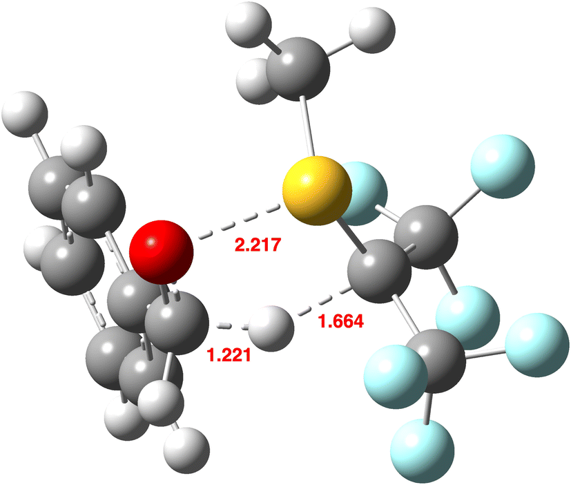
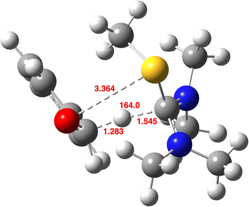
Before proceeding to discuss the isotope effects present in the reactions of 2 and 3, we address the relative magnitudes of k_invvs. k_1–4 (S_(R)/(S) or endo–exo isomerism) and of k₀vs. k_1–4 (Scheme 1, R = H) for the two reactions preceding the final hydrogen transfers.

The first aspect is modelling the transition structure³² for the initial proton abstraction from 1 by base (k₀ in Scheme 1). Using trimethylamine as the base (Fig. 1) resulted in an activation free energy (B3LYP+GD3+BJ/Def2-TZVPP/SCRF(DCM)) of +14.8 kcal mol⁻¹. To compare this energy with that of the subsequent reactions of 2 and 3, two models were investigated. The first is a supermolecule³³ of the exo-TS containing a hydrogen-bond bound Me₃NH⁺·Cl⁻, which emerged as 7.1 kcal mol⁻¹ lower than the initial proton abstraction step k₀. The second is an additive model of the exo-TS in which the free energy of Me₃NH⁺·Cl⁻ is added³⁴ to that of the exo-TS and this emerges as 10.5 kcal mol⁻¹ lower. This result supports the claim⁹ that k₀ is the slow step in the overall reaction and that the reactions k_1–4 represent faster intramolecular reactions. We also note that the formation of 1 itself has some interesting stereochemical features.³⁵ The second aspect is the process connecting the endo- and exo-transition structures (k_inv, Scheme 1). First, we note that the reversible proton transfers connecting species 1 with 2 or 3 (Scheme 1) serve as such a mechanism, noting previously that this process is higher in free energy than reactions k_1–4 themselves. One cannot yet exclude the possibility that the energy of the transition structure³⁶ for direct S-inversion may be lower than those for reactions k_1–4. A B3LYP+GD3+BJ/Def2-TZVPP/SCRF = dichloromethane model (Fig. 2) shows that ΔG is 30.5 kcal mol⁻¹ higher than the resulting exo-TS³⁷ and 20.0 kcal mol⁻¹ higher than the transition structure for initial proton abstraction. Hence for both possibilities we infer that k_inv « k₁–k₄. The rate of this isomerisation is therefore insignificant compared to the subsequent intramolecular hydrogen transfers, and only the rate model assuming forbidden inversion⁹ was investigated further (see eqn (1)).

Fig. 1 Calculated transition structure³² for initial deprotonation (k₀) showing the displacement vector and selected bond lengths in Å.

Fig. 2 Calculated transition structure³⁶ for inversion at sulfur (k_inv), showing the displacement vectors.

3.3 Conformations of species 2 and 3 (ref. 38)

Calculated coordinates for 2 and 3 (Scheme 1) are denoted as “ylide preceding endo-TS1” or “ylide preceding exo-TS1” respectively in the ESI.⁹ For a specific configuration at sulfur (e.g. (R)), they represent rotamers around the C–O bond (Fig. 3) if no isotopic substitution is present (Scheme 1, X = H). Species 2 (endo) has a C–O torsion angle of ∼10° and species 3 (exo) −165°. These represent the two lowest energy conformations, whilst two further minima are higher in energy (Fig. 3) and are not used here for calculation of KIEs. It is noteworthy that the rotation about the S–O bond is strongly coupled in a gear-like manner to the C–O rotation, so that both occur in synchrony (Fig. 3b). This strong coupling also causes the noise visible in Fig. 3b at dihedral angles of 100–200° due to inaccuracies in the internal coordinate geometry optimisations. In the original study, 2 was used as the reactant for computing KIEs for endo-TS1 and in our replication work, we followed the same procedure.

Fig. 3 (a) Calculated relative energy, in kcal mol⁻¹ (B3LYP+GD3+BJ/Def2-TZVPP/SCRF = DCM) of rotamers (R)-2 (X = H, Scheme 1) and the (R)-enantiomer of 3 (X = H) as a function of the 16S–15O torsion angle, and (b) calculated 12C–15O torsion angle as a function of rotation around the 16S–15O torsion angle.^39,40

3.4 Kinetic isotope effects for hydrogen transfer from 2 and 3

For the mechanism shown in Scheme 1 for which isotopic substitution X = D is present, the two stereochemical centres, on S and on the benzylic carbon, generates four stereochemical isomers, which occur as a pair of diastereomers and a pair of associated enantiomers. The two diastereomeric transition states are here labelled as endo-TS and exo-TS. The reactants for these transition states are 2 (endo) and 3 (exo), which are bond rotamers on the (non-isotopic) potential energy surface (Section 3.3). Kinetic isotope effects are computed for the reactions with rates k_1–4 as shown in Scheme 1, where k₂/k₁ is the protium/deuterium rate ratio for the endo-TS and k₄/k₃ for exo-TS. For the condition already established where k_inv « k₁–k₄ (“forbidden inversion”),⁹ the overall isotope effect combining the rates of both endo- and exo-transition structure reactions can be derived⁹ as:

Eqn (1) has the correct limiting form when the free energies of the two isomeric transition structures are identical, in which case the equalities k₃ = k₁ and k₄ = k₂ apply and hence eqn (1) reduces to eqn (2):

We note that eqn (2) in the original article⁹ is equivalent to eqn (1) above, but only if the labels are adopted as shown in Scheme 3 of the original article and specifically not from Scheme 4 of the original article, where k₃ and k₄ are transposed in error.⁹

A further test of the behaviour of eqn (1) can be set as e.g. k₂ = 3, and k₄ = 0.003, where the isotope effects are set as 3.0 for both endo- and exo-transition structure isomers, but where the k₁ and k₂ are both 10³ larger than k₃ and k₄, equivalent to ΔΔG₁₉₅ (exo–endo) – 2.677 kcal mol⁻¹. Inserting these values into eqn (1) reduces to 0.0024/0.0008 = 3.0 and the overall isotope effect remains the same as that of the individual but unequal contributions of endo-TS and exo-TS to the reaction. This behaviour contrasts with that reported⁹ for the dependence of the computed intramolecular KIE on the difference in electronic energies between the endo-TS and exo-TS, shown graphically in Fig. 4 in the original article⁹ and derived from eqn (2) quoted there. This shows an apparent strong dependency of KIEs on the relative energies (indicated as ΔE⁹) of the endo- and exo-transition structure isomers, with the value of the KIE reducing to a limiting value of unity (1.0) when ΔE > ±2 kcal mol⁻¹. At these two energy limits, the population and hence the rate for one isomer should entirely dominate and the other isomer would effectively make no contribution to the overall rate – the limiting value for the KIE derived from eqn (1) should correctly correspond to that of the dominant reaction isomer rather than to unity as previously claimed.⁹ To explore the difference between our analysis and the original,⁹ we have replotted the original Fig. 4⁹ in two ways as Fig. 4 here, one using labels defined from Scheme 4 of ref. 9 and one using eqn (1) as quoted in this article and labels shown in Scheme 1. We also used thermally corrected free energies (ΔΔG^‡) rather than electronic energy differences ΔE. These results are shown in Fig. 4a–c below.

Fig. 4 Plots derived from our eqn (1) shown as (a)–(h) and shown as (i) to (p) deriving from the literature⁹eqn (2) as defined from Scheme 4. In (a), the following sets of ratios for and respectively are (a) 2.2/2.2, (b) 2.1/2.3, (c) 2.0/2.4, (d) 1.9/2.5, (e) 1.8/2.6, (f) 1.7/2.7, (g) 1.6/2.8, and (h) 1.5/2.9 with the same ratios also used in plots (i) to (p) and with ΔΔG^‡ evaluated for a temperature of 250.15 K throughout. In (b), the ratios are now (a) 2.8/2.8, (b) 2.7/2.9, (c) 2.6/3.0, (d) 2.5/3.1, (e) 2.4/3.2, (f) 2.3/3.3, (g) 2.2/3.4, and (h) 2.1/3.5 and similarly for (i) to (p) using a temperature of 195.15 K throughout to derive ΔΔG^‡. (c) Uses the same values as (b), but is shown as an expansion of the region ΔΔG^‡ ±0.5 kcal mol⁻¹ centred at ΔΔG^‡ 0.0 kcal mol⁻¹.

Using eqn (1) as defined in Scheme 1 above, the correct limiting behaviour is now obtained (Fig. 4a–c), with large (>3.0 kcal mol⁻¹) free energy differences for the two isomeric transition structures reducing to either or rather than to unity as obtained in the original plot.⁹ For differences of ΔΔG^‡ <±0.5 kcal mol⁻¹ (approximately the values obtained from the computational modelling of this reaction), the dependency of the KIE is ∼linear, corresponding effectively to a Boltzmann weighted average of the individual values of and .

To calculate the isotope rate ratios and computationally for calculated transition structures, we require the calculated normal mode wavenumbers as applied to the Bigeleisen equation.⁴¹ These equations are given in the ESI for the original article,⁹ but the code used to evaluate these equations is neither noted nor provided there and the normal mode wavenumbers used as input to the code are also not included. Here we use the Kinisot program,⁴² which was based on a much earlier implementation of the Bigeleisen equation.^43,44 The KIEs are computed with the first term of the Bell tunnelling correction and a frequency scaling factor of 0.9806 for the 6-31+G(d,p) basis set.⁹ Details of all the KIE calculations are included as 73 examples, identified using the metadata search outlined in the Data availability and discovery section below.

3.4.1 Overall KIE computed using eqn (1). Our start point was gas phase transition structure models (for which no experimental values are available) for endo-TS and exo-TS, for which we have now established essentially exact replication between Gaussian 16 and Gaussian 03.⁴⁵ The KIE for the individual (endo) and (exo) ratios are here computed to be respectively 2.1855 and 2.2560@195 K. The values quoted⁹ are 2.19 and 2.26 respectively, which provides assurance that the Bigeleisen equation, vibrational scaling and tunnelling corrections have all been independently implemented in the same way for both studies. This congruence also confirms that the quoted values were indeed obtained for the gas phase at 195 K, since this condition was not explicitly stated.⁹ The free energy difference ΔΔG indicates an exo/endo ratio of 6.275 and implementing these values into eqn (1) gives a combined KIE₁₉₅ = 2.22, which is essentially the simple mean of the endo/exo values (see Fig. 3).

For dichloromethane solvent and the B3LYP/6-31+G(d,p) model, the computed (endo) and (exo) KIE ratios at 250 K are 1.660 (ref. 46) and 1.679 (ref. 47) (Lit. 1.62 and 1.72, Table 4 of ref. 9) using Gaussian 03 solvation models and at 195 K they are 1.907 (ref. 46) and 1.938 (ref. 47) (Lit. 1.85 and 1.72; the temperature was not stated, but is here inferred⁹). Using a value of ΔΔG₁₉₅ = 0.495 kcal mol⁻¹ gives the ratio of k₄/k₂ as 3.59 and combining this value with and as quoted above and applying eqn (1) gives KIE₁₉₅ = 1.922. The reported literature calculated value was KIE₁₉₅ = 1.63 (ref. 9, p 8093). In our present work, using a computed value of k₄/k₂ = 3.45, but using the reported⁹ but inappropriate total energy difference ΔE rather than the more appropriate free energy difference ΔΔG, together with quoted values of 1.85 and 1.72 (ref. 9) and finally applying eqn (1), we derive a value of KIE₁₉₅ = 1.783. Regardless of this relatively modest variation between the various predicted values of KIE₁₉₅ = 1.922, 1.63 (ref. 9) or 1.783, these values are all substantially lower than the measured KIE₁₉₅ of 2.82 ± 0.07, an observation that was propagated into the original article title⁹ as a significant deviation from transition structure theory.

We next investigate if this deviation can instead be attributed to deficiencies in the computational model.

3.5 Basis-set and density functional dependencies

We explored method dependency using only the endo-TS series (Table 1) by evaluating different pairs of density functional theory (DFT) functionals and basis sets and one semi-empirical method and using the more recent Gaussian 16 solvation models rather than replicating G03 parameters. The semi-empirical PM7 procedure (Table 1) predicts that KIE₂₅₀ is significantly larger (2.396 in dichloromethane) than that measured experimentally (2.08 ± 0.07), but with an associated tunnelling correction at lower temperatures that is vastly over-estimated using the Bell term. The transition structure at this level has an S–O bond that is still largely intact (r_S–O = 1.799 Å), with a relatively symmetrical but non-linear proton transfer (r_C–H 1.407/1.477 Å, α_CHC 128.3°). An error in the opposite direction is obtained using the B3LYP/Def2-SVP and B3LYP/Def2-SVPP split valence/double-ζ basis methods⁴⁸ (approximately equivalent to the original 6-31+G(d,p) basis) in dichloromethane and using an estimated vibrational scale factor of 0.97, the KIE₂₅₀ (endo) values are 1.53 and 1.51 respectively. These results are even worse than the KIE₂₅₀ obtained from the originally calculated B3LYP/6-31+G(d,p) model using Gaussian 03 (1.62, Table 4 of ref. 9) or here replicated using the Gaussian 16 solvation model (1.686). The geometries of the transition structures at these levels are significantly different from the PM7 result, showing a more advanced S–O bond cleavage (r_S–O 2.24–2.29 Å) and a less advanced and hence asymmetrical proton transfer (r_C–H ∼ 1.19/1.86 Å, α_CHC 137–138°), which results in a lower predicted isotope effect.

Table 1 Calculated kinetic isotope effects for hydrogen transfer from 2 to give 4/5 via the endo-TS

Method	Solvent	ΔG^‡298, kcal mol^−1	ν i , cm^−1	KIE
				195 K	210 K	226 K	250 K
a Using rotamer 3 as shown in Fig. 3. b Using rotamer 2 as shown in Fig. 3. All entries not indicated use rotamer 2. Full energies and coordinates can be obtained from a FAIR version of this table^54via 3D interactive models.
B3LYP/6-31+G(d,p)	Carbon tetrachloride	4.891	−337.50	2.078	1.975	1.885	1.777
	Chlorobenzene	4.276	−299.40	1.976	1.885	1.805	1.709
	Chloroform	4.369	−305.76	1.994	1.901	1.819	1.721
	Dichloromethane	4.079	−287.04	1.942	1.855	1.778	1.686
	Dichloroethane	4.027	−284.25	1.935	1.848	1.772	1.681
B3LYP/Def2-SVP	Dichloromethane	3.631	−312.58	1.704	1.643	1.589	1.525
B3LYP/Def2-SVPP	Dichloromethane	3.242	−313.78	1.686	1.627	1.575	1.512
B3LYP/Def2-TZVPP	Carbon tetrachloride	8.732	−459.64	2.749	2.557	2.392	2.201
	Chlorobenzene	8.400	−421.92	2.598	2.427	2.281	2.109
	Chloroform	8.385	−428.26	2.623	2.449	2.299	2.124
	Dichloromethane	7.969	−409.63	2.546	2.383	2.242	2.077
	Dichloroethane	7.834	−406.84	2.534	2.373	2.233	2.070
B3LYP/Def2-QZVPP	Carbon tetrachloride	9.537	−464.72	2.888	2.675	2.494	2.284
	Chlorobenzene	8.478	−425.19	2.697	2.512	2.354	2.170
	Chloroform	8.732	−431.85	2.727	2.538	2.377	2.188
	Dichloromethane	7.971	−412.35	2.641	2.464	2.313	2.136
	Dichloroethane	7.849	−409.44	2.628	2.454	2.304	2.128
B3LYP+GD3+BJ/Def2-QZVPP (endo-TS)	Dichloromethane (IEFPCM)	6.720	−405.65	2.598^a	2.426	2.279	2.106
				2.536^b	2.372	2.232	2.066
	Dichloromethane (CPCM)	6.926	−399.14	2.510	2.350	2.212	2.050
B3LYP+GD3+BJ/Def2-QZVPP (exo-TS)	Dichloromethane	6.411	−400.40	2.704	2.517	2.357	2.171
ωB97X-D/Def2-TZVPP	Carbon tetrachloride	10.179	−601.52	3.144	2.871	2.648	2.400
	Chlorobenzene	9.403	−549.34	2.782	2.576	2.403	2.206
	Chloroform	9.540	−557.69	2.830	2.616	2.437	2.233
	Dichloromethane	9.136	−532.74	2.696	2.505	2.343	2.157
	Dichloroethane	9.067	−529.39	2.680	2.491	2.332	2.148
ωB97X-D/Def2-QZVPP	Carbon tetrachloride	10.455	−605.25	3.297	2.998	2.756	2.487
	Chlorobenzene	11.170	−551.97	3.042	2.797	2.593	2.361
	Chloroform	9.904	−560.62	2.958	2.724	2.530	2.309
	Dichloromethane	9.783	−535.57	2.950	2.722	2.530	2.311
	Dichloroethane	9.686	−531.52	2.931	2.706	2.517	2.300
B2PLYP-D3/Def2-TZVPP	Carbon tetrachloride	5.464	−469.08	2.716	2.528	2.368	2.181
	Chlorobenzene	4.867	−442.10	2.620	2.446	2.297	2.124
	Chloroform	4.932	−446.48	2.633	2.458	2.307	2.132
	Dichloromethane	6.622	−433.38	2.596	2.426	2.280	2.109
	Dichloroethane	6.445	−432.01	2.595	2.425	2.279	2.109
B2PLYP-D3/Def2-QZVPP (endo-TS)	Dichloromethane	6.687	−433.62	2.770^a	2.574	2.407	2.213
				2.776^b	2.579	2.411	2.215
B2PLYP-D3/Def2-QZVPP (exo-TS)	Dichloromethane	6.235	−427.67	2.874	2.664	2.485	2.276
PM7 (semi-empirical)	Carbon tetrachloride	29.609	−1630.4	24.738	10.021	5.791	3.033
	Chlorobenzene	27.547	−1605.0	17.172	7.904	4.714	2.453
	Chloroform	29.156	−1608.5	20.775	9.314	5.476	2.815
	Dichloromethane	27.539	−1598.1	16.506	7.757	4.640	2.396

---

We next investigated how dependent these results are on the basis set. KIE₂₅₀ (endo) obtained from a B3LYP/Def2-TZVPP triple-ζ level model⁴⁸ agrees far better with the experimentally measured KIE₂₅₀ for the solvent range carbon tetrachloride (exp 2.17 ± 0.04, calc 2.20), chlorobenzene (exp 2.14, calc 2.11), dichloromethane (2.08 ± 0.07, calc 2.08) and dichloroethane (exp 2.08, calc 2.07) (Table 1). At the B3LYP/Def2-QZVPP level,⁴⁸ where the basis set may be assumed to be approaching the complete basis set (CBS) limit, results such as dichloromethane (KIE₂₅₀ 2.08 ± 0.07, calc 2.136) suggest that the method is now slightly overshooting the experiment, but this overshoot is reduced (KIE₂₅₀ 2.08 ± 0.07, calc 2.066) when a third-generation dispersion correction⁴⁹ is added to the method (Fig. 5).⁵⁰ Another method which includes a second-generation dispersion correction (ωB97X-D/Def2-QZVPP)⁵¹ over-estimates the KIE₂₅₀ (2.08 ± 0.07, calc 2.311). We also note that the results are relatively insensitive to the precise solvation model used (IEFPCM vs. CPCM, Table 1).

Fig. 5 Calculated geometry of the endo-TS at the B3LYP+GD3+BJ/Def2-QZVPP/SRCF = dichloromethane level with selected bond lengths in Å.

Our final and computationally the most expensive procedure is the double-hybrid B2PLYP-D3 (ref. 52)/Def2-QZVPP method which includes dispersion and correlation corrections at several levels. The transition structure geometry⁵³ is similar to the previous methods (r_S–O 2.264 Å, r_C–H 1.19/1.71 Å, α_CHC 140°) and results in the following values of KIE for endo: 2.215@250 K and 2.776@195 K and for exo: 2.276@250 K and 2.874 @195 K. The calculated exo/endo ratios are respectively 2.47@195 K and 2.22@250 K. When the individual KIEs are combined using eqn (1), KIE = 2.245@250 K and 2.824@195 K, compared to experimental values of 2.08 ± 0.07@250 K and 2.82 ± 0.06@195 K. We discuss temperature effects on the kinetic isotope effects below.

3.6 Explicit solvation models

In this section, we investigate an apparent outlier in the reported experimental KIE values in chloroform as solvent, 1.98 vs. 2.08–2.17 for aprotic solvents @250 K. There was no supporting evidence for this anomaly from the continuum solvent model calculations (Table 1). Chloroform, unlike the other solvents, has the ability to form weak hydrogen bonds and this suggests that we may have to consider solvent models in which one or more explicit molecules supplement the continuum solvent. A model including just one chloroform hydrogen-bonded to oxygen (Fig. 6) shows a KIE₂₅₀ reduced to 1.953 relative to the value with no chloroform of 2.124 (B3LYP/Def2-TZVPP). The value reduces further to 1.758 if a third-generation dispersion correction model such as B3LYP+GD3+BJ/Def2-TZVPP is used and becomes KIE₂₅₀ = 1.800 at the Def2-QZVPP basis set level (Table 2). A very approximate estimate is that the experimental KIE can be reproduced using a computed model containing 68% substrate with no H-bonded solvent and 32% with one explicit solvent, corresponding to an equilibrium with ΔG ∼ +0.4 kcal mol⁻¹. The difference in calculated free energy of the combined molecule compared to the isolated components is rather larger at +2.7 kcal mol⁻¹, but it is suggestive that such a composite model containing a modest proportion of discrete hydrogen-bonded chloroform solvation could explain the reduced experimental KIE.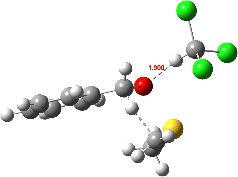

Fig. 6 Calculated geometry of the endo-TS containing one explicit solvent molecule at the B3LYP+GD3+BJ/Def2-QZVPP/SRCF = dichloromethane level,⁵⁵ with selected bond lengths in Å.

Table 2 Calculated kinetic isotope effects for the reaction of 2via endo-TS, with inclusion of one explicit chloroform solvent molecule

Method	ΔG^‡, kcal mol^−1	ν i , cm^−1	KIE
			195 K	210 K	226 K	250 K
B3LYP/Def2-TZVPP	4.67	−381.45	2.349	2.212	2.093	1.953
B3LYP+GD3+BJ/Def2-TZVPP	5.48	−351.08	2.049	1.949	1.862	1.758
B3LYP+GD3+BJ/Def2-QZVPP	5.61	−353.89	2.114	2.006	1.912	1.800

---

3.7 Temperature variation of the kinetic isotope effect

Another outlier apparent in the original report is the temperature variation of the KIE in dichloromethane as solvent. The original Arrhenius plot (Fig. 7 of article⁹), recalculated below as an Eyring plot (Fig. 7), can be re-interpreted as showing linear behaviour for the experimental values between 250 and 210 K and an outlying value at 195 K. In contrast, all the various computed models discussed (Tables 1 and 2) above show linear behaviour across the entire temperature range. Ostensibly, the experimental value at 195 K could indicate a relatively abrupt increase in tunnelling to explain the unexpectedly large value of the KIE at this temperature; a linear extrapolation would suggest that the observed value should only be reached at ∼172 K. Only further experimental analysis exploring the KIE in the region surrounding 195–210 K would resolve whether this is a fascinating real effect or an experimental artefact. More sophisticated tunnelling models involved could also help resolve this aspect,⁵⁶ which we will be exploring in future work. We may reasonably conclude from the clustering of the calculated isotope effects around or above the experiment points (Fig. 7) that the transition state model largely remains robust. The observation that the predicted magnitudes of the KIE are slightly larger than those measured may also be associated with the use of theory based on a harmonic oscillator model, whereas the observed values are associated with anharmonic vibrational effects.

Fig. 7 Eyring plots of the computationally determined intramolecular deuterium KIEs computed at (1) B3LYP/6-31+G(d,p) (Gaussian 16), (2) B3LYP/6-31+G(d,p) (Gaussian 03), (3) B3LYP/Def2-SVP, (4) B3LYP/Def2-SVPP (a) and (5) B3LYP/Def2-TZVPP, (6) B3LYP/Def2-QZVPP, (7) ωB97X-D/Def2-TZVPP, (8) ωB97X-D/Def2-QZVPP, (9) B2PLYP-D3/Def2-TZVPP, (10) B2PLYP-D3/Def2-QZVPP, (11) B3LYP+GD3+BJ/Def2-QZVPP (IEFPCM), and (12) B3LYP+GD3+BJ/Def2-QZVPP (CPCM) (b). (Exp.) experimental results with uncertainties indicated by shading.

3.8 Substituent effects⁵⁷

Three substituents at the extremes of electron donation and withdrawal were selected to probe how the kinetic isotope was affected: R = NO₂, NMe₂ and CF₃ (Scheme 1 and Table 3).

Table 3 Calculated kinetic isotope effects for substituted derivatives of 2 for dichloromethane as solvent

Method	ΔG^‡, kcal mol^−1	ν i , cm^−1	KIE
			195 K	210 K	226 K	250 K
B3LYP+GD3BJ/Def2-TZVPP; R = NMe2	6.28	−716.29	7.757	6.229	5.246	4.322
B3LYP+GD3BJ/Def2-QZVPP; R = NMe2	6.44	−764.53	10.055	7.389	5.965	4.760
B3LYP+GD3BJ/Def2-TZVPP; R = CF3	18.86	−559.79	3.661	3.320	3.039	2.724
B3LYP+GD3BJ/Def2-QZVPP; R = CF3	19.77	−569.05	3.852	3.476	3.170	2.828
B3LYP+GD3BJ/Def2-QZVPP; R = NO2	27.23	−668.78	4.420	3.889	3.486	3.059

---

For R = CF₃,⁵⁸ the transition structure geometry (Fig. 8) shows a more compact and more symmetrical and linear hydrogen-transfer centre compared to R = H (Fig. 5). These factors combine to increase the predicted value KIE₁₉₅ for R = CF₃ to 3.852, compared to 2.51 at the same level for R = H. The substituents R = NO₂ further increase this trend.

Fig. 8 Calculated geometry of the endo-TS, R = CF₃ at the B3LYP+GD3+BJ/Def2-QZVPP/SRCF = dichloromethane level,⁵⁸ with selected bond lengths in Å.

An even larger effect is seen for R = NMe₂ (Fig. 9),⁵⁹ with the S–O bond now largely broken at the transition structure and the reaction comprising an almost pure and more symmetrical hydrogen transfer with the angle at the transferring centre now approaching linearity.

Fig. 9 Calculated geometry of the endo-TS, R = NMe₂ at the B3LYP+GD3+BJ/Def2-QZVPP/SRCF = dichloromethane level,⁵⁹ with selected bond lengths in Å.

These properties all combine to further increase the predicted value of KIE₁₉₅ for R = NMe₂ to 10.1, of which a factor of 1.46 is now due to larger tunnelling contributions associated with the larger value of v_l 765 cm⁻¹. Whilst these specific substituents may not be synthetically feasible, we have at least established a consistent method for predicting isotope effects for new substituents located at any position in the substrates and hence for designing variations on Swern oxidation that could sustain larger deuterium kinetic isotope effects.

4 Conclusions

The first aim here was to replicate an earlier study⁹ reporting calculated kinetic isotope effects for the key hydrogen transfer step in the Swern oxidation of an alcohol to an aldehyde, conducted some 13 years ago using an earlier version of the Gaussian program, G03. For the gas phase model, the replication was essentially exact. The task proved more complex when a continuum solvation model was included. Although the latest version G16 has keywords that aim to reproduce the solvation model and other parameters used in G03, using this approach resulted in significant energy gradients when the original geometry was tested. There were also uncertainties relating to the transition structure coordinates deposited as part of the original modelling of kinetic isotope effects⁹ and whether they related to their optimisation in a gas phase or solvent-continuum environment. Because no original vibrational analysis was included in the ESI, we had to re-optimise these geometries to obtain the essential input into the Bigeleisen equation used to predict the kinetic isotope effects (KIEs). This replication was less accurate but did not alter the original conclusion that the values of the isotope effects were predicted to be significantly smaller than those experimentally measured – a result that was described⁹ as a significant deviation from transition state theory for this reaction.

In this work, we can now attribute this result to a significant basis-set dependence of the calculations, both on the computed geometry of the transition structure and the resulting vibrational analysis on which the kinetic isotope effects are based. Identifying the root cause of why KIE values are underestimated when a small basis set is used for this specific reaction will be performed in a follow-up study, but we speculate here that it may be at least in part associated with the very non-linear nature of the hydrogen transfer and the inability of a small basis set to accurately describe the normal modes at such geometries. Other origins of tunnelling instability in pericyclic reactions have recently been suggested.⁶⁰ We find that factors such as the continuum solvation model or the selection of a density functional method were less sensitive. We also note that inclusion of an empirical term to correct for dispersion attractions did have a moderate effect on the computed KIE values, as did the inclusion of an explicit solvent model for solvents where a hydrogen bond between the solvent and the substrate becomes possible. Our best suggested procedure, maximising accuracy whilst reducing computation times to a practical level, is at the B3LYP/Def-QZVPP level as corrected for third generation dispersion attractions and using a continuum solvation model.

We have utilized this model to predict KIEs for two new substituents, finding one of them (R = NMe₂) to significantly increase the isotope effects, achieved with minimal effect on the computed reaction barriers.

As an aid to any future replication of our own results, we include many links to the FAIR data archives for our calculations in the form of citations in the article bibliography, noting that our data files are not handled by error-prone humans but are produced by automated machine workflows. The citations noted here are included in the metadata record for the article, which is registered with CrossRef,⁶¹ albeit with one significant current limitation in that there is currently no formal declaration of these citations as specific pointers to a FAIR data collection. Such data citations could be included in knowledge graphs,⁶² facilitating the mapping of connections between conclusions drawn in an article and the data on which these conclusions are based.

Data availability and discovery statement

Available as a FAIR and AI-ready Imperial College Research Data Repository accessible viahttps://doi.org/10.14469/hpc/13058 for the overall collection and findable by following the hierarchy of data collections identified there. The data discovery and accessibility aspects are further enabled by using one of the following two methods: (1) discovery using a metadata search query. An example template for identifying kinetic isotope data deriving from a Gaussian calculation is here provided as: https://commons.datacite.org/?query=media.media_type:chemical/x-gaussian-log+AND+media.media_type:text/plain+AND+(titles.title:*Exo*+OR+titles.title:*Endo*). This query can be modified or extended as required.⁶³ (2) Discovery using an enhancement of Table 1,⁵⁴https://doi.org/10.14469/hpc/13370 acting as a data Finding Aid via links to data collections associated with each row of Table 1 and including a visual tool for displaying interactive 3D coordinate models illustrating the transition structure normal vibrational modes. This model is interactively created by re-using data accessed using information in the metadata record associated with the FAIR DOI of each dataset.

Conflicts of interest

There are no conflicts to declare.

Acknowledgements

SL thanks the IROP (International Research Opportunities Program) for a grant supporting this undergraduate research visit to Imperial College London from the University of Toronto in 2023.

References

1. D. C. Braddock, N. Limpaitoon, K. Oliwa, D. O'Reilly, H. S. Rzepa and H. A. J. P. White, A Stereoselective Hydride Transfer Reaction with contributions from Attractive Dispersion Force Control, Chem. Commun., 2022, 58, 4981–4984,  10.1039/D2CC01136K.
2. H. Okamura, Y. Yasuno, A. Nakayama, K. Kumadaki, K. Kitsuwa, K. Ozawa, Y. Tamura, Y. Yamamoto and T. Shinada, Selective oxidation of alcohol-d₁ to aldehyde-d₁ using MnO₂, RSC Adv., 2021, 11, 28530–28534,  10.1039/D1RA05405H.
3. R. D. Kardile and R.-S. Liu, Two Distinct Ag(I)- and Au(I)-Catalyzed Olefinations between α-Diazo Esters and N-Boc-Derived Imines, Org. Lett., 2019, 21, 6452–6456,  DOI:10.1021/acs.orglett.9b02343.
4. A. S. Kulandai Raj, A. S. Narode and R.-S. Liu, Gold(I)-Catalyzed Reactions between N-(o-Alkynylphenyl)imines and Vinyldiazo Ketones to Form 3-(Furan-2-ylmethyl)-1H-indoles via Postulated Azallyl Gold and Allylic Cation Intermediates, Org. Lett., 2021, 23, 1378–1382,  DOI:10.1021/acs.orglett.1c00038.
5. For an excellent overview of pre-existing methods of deuterated aldehyde synthesis and for RCDO preparation directly from RCHO, see: H. Geng, X. Chen, J. Gui, Y. Zhang, Z. Shen, P. Qian, J. Chen, S. Zhang and W. Wang, Practical synthesis of C1 deuterated aldehydes enabled by NHC catalysis, Nat. Catal., 2019, 2, 1071–1077,  DOI:10.1038/s41929-019-0370-z.
6. For a recent review see: Y. Guo, Z. Zhuang, Y. Liu, X. Yang, C. Tan, X. Zhao and J. Tan, Advances in C₁-deuterated aldehyde synthesis, Coord. Chem. Rev., 2022, 263, 214525,  DOI:10.1016/j.ccr.2022.214525.
7. K. Omura and D. Swern, Oxidation of alcohols by ‘activated’ dimethyl sulfoxide. A preparative, steric and mechanistic study, Tetrahedron, 1978, 34, 1651–1660,  DOI:10.1016/0040-4020(78)80197-5.
8. A. J. Mancuso and D. Swern, Activated dimethyl sulfoxide: useful reagents for synthesis, Synthesis, 1981, 165–185,  DOI:10.1055/s-1981-29377.
9. T. Giagou and M. P. Meyer, Mechanism of the Swern Oxidation: Significant Deviations from transition structure Theory, J. Org. Chem., 2010, 75, 8088–8099,  DOI:10.1021/jo101636w.
10. For a preprint, see, D. C. Braddock, S. Lee and H. S. Rzepa, SWERN Oxidation. transition structure Theory is OK, ChemRxiv, 2023, preprint,  DOI:10.26434/chemrxiv-2023-vcmcl.
11. M. J. Frisch, G. W. Trucks, H. B. Schlegel, G. E. Scuseria, M. A. Robb, J. R. Cheeseman, G. Scalmani, V. Barone, G. A. Petersson, H. Nakatsuji, X. Li, M. Caricato, A. V. Marenich, J. Bloino, B. G. Janesko, R. Gomperts, B. Mennucci, H. P. Hratchian, J. V. Ortiz, A. F. Izmaylov, J. L. Sonnenberg, D. Williams-Young, F. Ding, F. Lipparini, F. Egidi, J. Goings, B. Peng, A. Petrone, T. Henderson, D. Ranasinghe, V. G. Zakrzewski, J. Gao, N. Rega, G. Zheng, W. Liang, M. Hada, M. Ehara, K. Toyota, R. Fukuda, J. Hasegawa, M. Ishida, T. Nakajima, Y. Honda, O. Kitao, H. Nakai, T. Vreven, K. Throssell, J. A. Montgomery Jr, J. E. Peralta, F. Ogliaro, M. J. Bearpark, J. J. Heyd, E. N. Brothers, K. N. Kudin, V. N. Staroverov, T. A. Keith, R. Kobayashi, J. Normand, K. Raghavachari, A. P. Rendell, J. C. Burant, S. S. Iyengar, J. Tomasi, M. Cossi, J. M. Millam, M. Klene, C. Adamo, R. Cammi, J. W. Ochterski, R. L. Martin, K. Morokuma, O. Farkas, J. B. Foresman and D. J. Fox, Gaussian 16, Revisions C.01 and C.02, Gaussian, Inc., Wallingford CT, 2016.
12. R. Dennington, T. A. Keith and J. M. Millam, GaussView, Version 6.1, Semichem Inc., Shawnee Mission, KS, 2016.
13. M. Wilkinson, M. Dumontier and I. Aalbersberg, et al., The FAIR Guiding Principles for scientific data management and stewardship, Sci. Data, 2016, 3, 160018,  DOI:10.1038/sdata.2016.18.
14. M. J. Harvey, A. McLean and H. S. Rzepa, A metadata-driven approach to data repository design, J. Cheminf., 2017, 9, 4,  DOI:10.1186/s13321-017-0190-6.
15. H. S. Rzepa, The long and winding road towards FAIR data as an integral component of the computational modelling and dissemination of Chemistry, Isr. J. Chem., 2022, 62, e202100034–e202100034,  DOI:10.1002/ijch.202100034.
16. H. S. Rzepa, Teaching FAIR in Computational Chemistry: Managing and publishing data using the twin tools of Compute Portals and Repositories, Can. J. Chem., 2023, 101, 725–733,  DOI:10.1139/cjc-2022-0255.
17. H. S. Rzepa, Quantum chemistry interoperability (library): another step towards FAIR data, Chemistry with a Twist blog, 2022,  DOI:10.59350/mzs83-g6218.
18. C. Cave-Ayland, M. Bearpark, C. Romain and H. S. Rzepa, CHAMP is an HPC Access and Metadata Portal, J. Open Source Softw., 2022, 7, 3824,  DOI:10.21105/joss.03824.
19. D. C. Braddock, H. S. Rzepa and S. Lee, Imperial College Research Data Repository, 2023,  DOI:10.14469/hpc/13108.
20. D. C. Braddock, H. S. Rzepa and S. Lee, Imperial College Research Data Repository, 2023,  DOI:10.14469/hpc/12407.
21. D. C. Braddock, H. S. Rzepa and S. Lee, Imperial College Research Data Repository, 2023,  DOI:10.14469/hpc/13239.
22. D. C. Braddock, H. S. Rzepa and S. Lee, Imperial College Research Data Repository, 2023,  DOI:10.14469/hpc/12902.
23. D. C. Braddock, H. S. Rzepa and S. Lee, Imperial College Research Data Repository, 2023,  DOI:10.14469/hpc/13176.
24. D. C. Braddock, H. S. Rzepa and S. Lee, Imperial College Research Data Repository, 2023,  DOI:10.14469/hpc/13177.
25. G. Scalmani and M. J. Frisch, Continuous surface charge polarizable continuum models of solvation. I. General formalism, J. Chem. Phys., 2010, 114110,  DOI:10.1063/1.3359469.
26. D. C. Braddock, H. S. Rzepa and S. Lee, Imperial College Research Data Repository, 2023,  DOI:10.14469/hpc/13186.
27. D. C. Braddock, H. S. Rzepa and S. Lee, Imperial College Research Data Repository, 2023,  DOI:10.14469/hpc/13188.
28. D. C. Braddock, H. S. Rzepa and S. Lee, Imperial College Research Data Repository, 2023,  DOI:10.14469/hpc/13223.
29. D. C. Braddock, H. S. Rzepa and S. Lee, Imperial College Research Data Repository, 2023,  DOI:10.14469/hpc/13242.
30. D. C. Braddock, H. S. Rzepa and S. Lee, Imperial College Research Data Repository, 2023,  DOI:10.14469/hpc/13225.
31. D. C. Braddock, H. S. Rzepa and S. Lee, Imperial College Research Data Repository, 2023,  DOI:10.14469/hpc/13246.
32. D. C. Braddock, H. S. Rzepa and S. Lee, Imperial College Research Data Repository, 2023,  DOI:10.14469/hpc/13084.
33. D. C. Braddock, H. S. Rzepa and S. Lee, Imperial College Research Data Repository, 2023,  DOI:10.14469/hpc/12396.
34. D. C. Braddock, H. S. Rzepa and S. Lee, Imperial College Research Data Repository, 2023,  DOI:10.14469/hpc/13090.
35. H. S. Rzepa, Pre-mechanism for the Swern Oxidation: formation of chlorodimethylsulfonium chloride, Chemistry with a twist blog, 2023 DOI:10.59350/vmtgs-0gw62.
36. D. C. Braddock, H. S. Rzepa and S. Lee, Imperial College Research Data Repository, 2023,  DOI:10.14469/hpc/12404.
37. D. C. Braddock, H. S. Rzepa and S. Lee, Imperial College Research Data Repository, 2023,  DOI:10.14469/hpc/12379.
38. D. C. Braddock, H. S. Rzepa and S. Lee, Imperial College Research Data Repository, 2023,  DOI:10.14469/hpc/13337.
39. D. C. Braddock, H. S. Rzepa and S. Lee, Imperial College Research Data Repository, 2023,  DOI:10.14469/hpc/13355.
40. D. C. Braddock, H. S. Rzepa and S. Lee, Imperial College Research Data Repository, 2023,  DOI:10.14469/hpc/13337.
41. J. Bigeleisen and M. G. Mayer, Calculation of Equilibrium Constants for Isotopic Exchange Reactions, J. Chem. Phys., 1947, 15, 261–267,  DOI:10.1063/1.1746492.
42. R. Paton, Kinisot, V2.0.1, Zenodo, 2022,  DOI:10.5281/zenodo.6831009.
43. H. S. Rzepa, KINISOT. A basic program to calculate kinetic isotope effects using normal coordinate analysis of transition structure and reactants, Zenodo, 2015,  DOI:10.5281/zenodo.19272.
44. S. B. Brown, M. J. S. Dewar, G. P. Ford, D. J. Nelson and H. S. Rzepa, Ground States of Molecules. MNDO Calculations of Kinetic Isotope Effects, J. Am. Chem. Soc., 1978, 100, 7832–7836,  DOI:10.1021/ja00493a008.
45. D. C. Braddock, H. S. Rzepa and S. Lee, Imperial College Research Data Repository, 2023,  DOI:10.14469/hpc/13256.
46. D. C. Braddock, H. S. Rzepa and S. Lee, Imperial College Research Data Repository, 2023,  DOI:10.14469/hpc/12902.
47. D. C. Braddock, H. S. Rzepa and S. Lee, Imperial College Research Data Repository, 2023,  DOI:10.14469/hpc/13189.
48. F. Weigend and R. Ahlrichs, Balanced basis sets of split valence, triple zeta valence and quadruple zeta valence quality for H to Rn: Design and assessment of accuracy, Phys. Chem. Chem. Phys., 2005, 7, 3297–3305,  10.1039/B508541A.
49. S. Grimme, S. Ehrlich and L. Goerigk, Effect of the damping function in dispersion corrected density functional theory, J. Comput. Chem., 2011, 32, 1456–1465,  DOI:10.1002/jcc.21759.
50. D. C. Braddock, H. S. Rzepa and S. Lee, Imperial College Research Data Repository, 2023,  DOI:10.14469/hpc/13261.
51. J.-D. Chai and M. Head-Gordon, Long-range corrected hybrid density functionals with damped atom-atom dispersion corrections, Phys. Chem. Chem. Phys., 2008, 10, 6615–6620,  10.1039/B810189B.
52. T. Schwabe and S. Grimme, Double-hybrid density functionals with long-range dispersion corrections: higher accuracy and extended applicability, Phys. Chem. Chem. Phys., 2007, 9, 3397,  10.1039/B704725H.
53. D. C. Braddock, H. S. Rzepa and S. Lee, Imperial College Research Data Repository, 2023,  DOI:10.14469/hpc/12928.
54. D. C. Braddock, H. S. Rzepa and S. Lee, Imperial College Research Data Repository, 2023,  DOI:10.14469/hpc/13370.
55. D. C. Braddock, H. S. Rzepa and S. Lee, Imperial College Research Data Repository, 2023,  DOI:10.14469/hpc/13276.
56. S. Hammes-Schiffer, Theoretical perspectives on non-Born–Oppenheimer effects in chemistry, Philos. Trans. R. Soc., A, 2022, 380, 20200377,  DOI:10.1098/rsta.2020.0377.
57. D. C. Braddock, H. S. Rzepa and S. Lee, Imperial College Research Data Repository, 2023,  DOI:10.14469/hpc/13327.
58. D. C. Braddock, H. S. Rzepa and S. Lee, Imperial College Research Data Repository, 2023,  DOI:10.14469/hpc/13326.
59. D. C. Braddock, H. S. Rzepa and S. Lee, Imperial College Research Data Repository, 2023,  DOI:10.14469/hpc/13320.
60. A. Frenklach, H. Amlani and S. Kozuch, J. Am. Chem. Soc., 2024, 146, 11823–11834,  DOI:10.1021/jacs.4c00608.
61. https://www.crossref.org, accessed 15/11/2023.
62. H. Cousijn, R. Braukmann, M. Fenner, C. Ferguson, R. van Horik, R. Lammey, A. Meadows and S. Lambert, Patterns, 2020, 2, 100180,  DOI:10.1016/j.patter.2020.100180.
63. Further examples can be found at e.g., H. S. Rzepa, Chemistry with a Twist Blog, 2020,  DOI:10.59350/7jq8v-z4p56.

---

Footnote

† Electronic supplementary information (ESI) available. See DOI: https://doi.org/10.1039/d3dd00246b

---