
 Open Access Article
 This Open Access Article is licensed under a
 Creative Commons Attribution 3.0 Unported Licence
Orientational anisotropy due to molecular field splitting in sulfur 2p photoemission from CS2 and SF6 – theoretical treatment and application to photoelectron recoil†
Edwin
Kukk
 *a,
Johannes
Niskanen
a,
Oksana
Travnikova
b,
Marta
Berholts
c,
Kuno
Kooser
c,
Dawei
Peng
b,
Iyas
Ismail
b,
Maria Novella
Piancastelli
b,
Ralph
Püttner
d,
Uwe
Hergerhahn
e and
Marc
Simon
b
*a,
Johannes
Niskanen
a,
Oksana
Travnikova
b,
Marta
Berholts
c,
Kuno
Kooser
c,
Dawei
Peng
b,
Iyas
Ismail
b,
Maria Novella
Piancastelli
b,
Ralph
Püttner
d,
Uwe
Hergerhahn
e and
Marc
Simon
b
aDepartment of Physics and Astronomy, University of Turku, FI-20014 Turku, Finland. E-mail: edwin.kukk@utu.fi
bSorbonne Université, CNRS, UMR 7614, Laboratoire de Chimie Physique-Matière et Rayonnement, F-75005 Paris, France
cInstitute of Physics, University of Tartu, W. Ostwaldi 1, EE-50411 Tartu, Estonia
dFachbereich Physik, Freie Universität Berlin, D-14195 Berlin, Germany
eFritz-Haber-Institut der Max-Planck-Gesellschaft, Faradayweg 4-6, 14195 Berlin, Germany
First published on 1st August 2024
Abstract
Photoelectron recoil strongly modifies the high kinetic energy photoemission spectra from atoms and molecules as well as from surface structures. In most cases studied so far, photoemission from atomic-like inner-shell or core orbitals has been assumed to be isotropic in the molecular frame of reference. However, in the presence of molecular field splitting of p or d orbitals, this assumption is not justified per se. We present a general theoretical treatment, linking the orientational distribution of gas-phase molecules to the electron emission and detection in a certain direction in the laboratory frame. The approach is then applied to the S 2p photoemission from a linear molecule such as CS2 and we investigate, how the predicted orientational anisotropies due to molecular field splitting affect the photoelectron recoil excitations. Lastly, experimental S 2p high-kinetic-energy photoelectron spectra of SF6 and CS2 are analyzed using the modeled recoil lineshapes representing the anisotropy-affected recoil effects.
1 Introduction
Atomic inner-shell photoemission spectroscopy is a powerful tool to probe the chemical surroundings and the photoinduced dynamics of atoms embedded in systems of various complexity, from diatomic molecules to polymers, liquids and crystalline solids. Photoelectron spectra contain information such as chemical shifts of peak energies from atoms in different chemical neighbourhood,1 broadenings of peaks due to core-hole lifetime2 and lineshape modifications due to post-collision interaction (PCI).3 The spectra also reveal the dynamic response of the system to photoabsorption, vibrational progressions seen in molecular inner-shell photoelectron spectra being a pertinent example.4 In particular, the so-called Franck–Condon excitations,5 resulting from a sudden change in the molecular potential energy surface when an electron is removed, are a common feature in molecular inner shell and core photoemission spectra and have been thoroughly studied.4,6,7In this work related specifically to hard X-ray high kinetic energy photoelectron spectroscopy (HAXPES), we will not concentrate on the above-mentioned features, but focus instead on a lesser-known feature of photoemission, the photoelectron recoil that becomes increasingly prominent at high kinetic energy.8–12 Near-threshold photoelectron spectra from literature (CS2, ref. 13) and from this experiment (SF6) were utilized to obtain underlying Franck–Condon excitation structure and other recoil-indepenent parameters for the HAXPES analysis; these must be included in order to separate them from the recoil effects, but are not a central feature of our study.
It has been established by a number of studies that the recoil features form an inseparable part of the photoelectron spectra of molecules and solids.8,14–23 Recoil results in energy loss and in the excitation of vibrational and rotational degrees of freedom, observable as vibrational progressions, line shifts and broadenings in the photoelectron spectra. The effects become so prominent (see, e.g., Fig. 1 in ref. 24) that any quantitative analysis of high-resolution inner-shell photoelectron spectra in the HAXPES regime should either include these effects or at least be mindful of them. Furthermore, since recoil excitations can access different vibrational modes than the Franck–Condon excitations, they explore hitherto unknown regions of the core-ionized molecular potential energy surface. These effects are also emitter-orientation-dependent, and have a potential of being an orientational probe.
The specific recoil excitations that take place depend on the photoemission direction in the molecular frame. For example, axial photoemission in diatomic molecules results in recoil-excited bond stretching vibrational excitations, whereas perpendicular photoemission recoil-excites molecular rotations only (transitional recoil is always present). However, in a typical single-molecule photoelectron spectroscopy experiment, the emitter molecules form a randomly oriented gas-phase ensemble, whereas the angle of the photoelectron detection is fixed relative to the propagation direction and polarization plane of the X-ray radiation.
The recoil excitations can be modeled in small molecules at a high level of accuracy. For inner-shell photoelectron spectroscopy, the model typically assumes that the recoil momentum is received initially by the emitter atom only and is distributed to the various degrees of freedom – translational, vibrational and rotational.12,16,25–27 The total recoil energy thus received is equal to that of the free emitter atom. Another assumption made in previous studies that dealt with 1s photoemission was that the molecules in the gas-phase ensemble that emitted the detected photoelectrons are oriented randomly and isotropically. In other words, the recoil direction in the molecular frame is isotropically distributed,17,28,29 which is equivalent to assuming an isotropic molecular-frame distribution for the core photoelectrons leaving the emitter atom. This is clearly an approximation as further intramolecular scattering, for example, can introduce anisotropy. Here, we extend these studies to the 2p inner-shell photoemission, which brings new considerations into the model.
The first difference from the 1s spectra is the presence of spin–orbit (s–o) splitting of the 2p orbital, into the 2p1/2 and 2p3/2 components, where the subscript denotes the j quantum number. Secondly, depending on the symmetry of the local environment, additional splitting can occur of the atomic 2p photoemission lines. Such a situation occurs when the atomic orbital is placed in a molecular field (MF) that has a sufficiently low symmetry so that the degeneracy of these orbitals is removed. For example, the 2p3/2 s–o component (doubly degenerate in the spherical symmetry of a free atom), is split into two components in linear molecules. The effect is referred to as the molecular field splitting.30 A feature of the MF splitting that is of particular interest for the present study is that the MF-split components of atomic orbitals are differently oriented in the molecular frame. This is indeed the prerequisite for their different energies in the MF.
Here, we combine the recoil model with the orientational anisotropy effects in the photoemission of gas-phase molecules. Specifically, we take advantage of the MF splitting to create such anisotropy in the CS2 S 2p emission, for which we develop a quantitative theoretical prediction. For reference and comparison purposes, the recoil effects are modeled also for the SF6 molecule that does not exhibit the MF splitting of S 2p and correspondingly has no anisotropy effects in photoelectron recoil. After this theoretical development, the recoil lineshapes (energy loss due to the recoil), incorporating the theoretically predicted orientational distributions, are calculated both for idealized and for the actual experimental conditions. Our result is then applied in least-squares analysis of the HAXPES spectra of S 2p in CS2, again with SF6 as a reference and comparison. Lastly, this analysis is compared with the theoretical prediction, it is discussed, to what extent the present state-of-art experiment can fully validate the model and what future improvements would be beneficial.
2 Theory – molecular orientation in photoemission and its effects on photoelectron recoil
Before one can specifically investigate the effect MF splitting has on photoelectron recoil, a much broader question must be addressed at the theoretical level. The angular distribution of atomic photoemission in the laboratory frame is a well-studied problem.31,32 However, here our question is different – namely, how does the anisotropy of the photoemission and the non-spherical symmetry of the bound electron's wavefunction translate into the anisotropy of the orientation of the gas-phase molecules that have emitted a photoelectron into a certain direction in the laboratory frame. We first present a general solution for this problem, proceeding then to the case of CS2. Then, we’ll review the essential features of the photoelectron recoil model, apply it to the specific cases of S 2p photoemission in CS2 and SF6 and finally, use the theoretical results obtained about the molecular orientation's anisotropy for refining the recoil model.2.1 Distribution of molecular orientations for a detected electron
We use an atom-in-a-molecule approach for photoionization in the special case where electron detection takes place along the linear polarization axis of the incident X-ray beam. We define this direction as the z-axis of the laboratory frame, from which the polar angle θ is measured. We define R to be the rotation that transforms the laboratory frame to the molecular one. Thus, the orientation of a molecule in a gas-phase ensemble is uniquely defined by R. Using Bayes's theorem, the probability p(R|e−) of the orientation R of the emitter molecule upon the detection of an electron e− is given by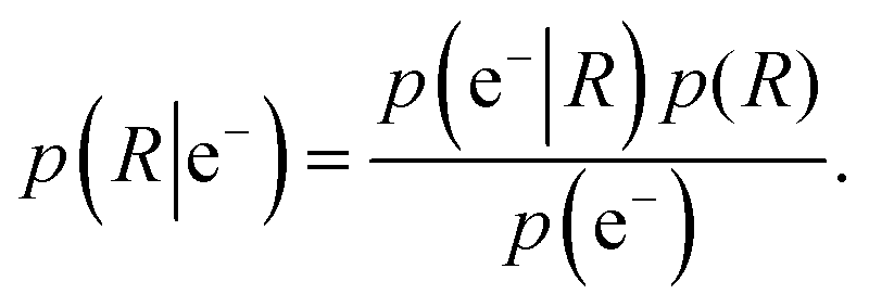 | (1) |
 | (2) |
![[thin space (1/6-em)]](https://www.rsc.org/images/entities/char_2009.gif) θ describes the relative probability of finding a molecule in a randomly oriented sample, with angle θ between the z-axes in the laboratory and molecular frames.
θ describes the relative probability of finding a molecule in a randomly oriented sample, with angle θ between the z-axes in the laboratory and molecular frames.
Let us narrow the case down to an inner-shell 2p photoionization in linear molecules, oriented along the z-axis of the molecular frame. For atomic-like S 2p photoionization, the inner-shell atomic orbitals split to s–o components, in which the quantum state i is characterized by the total quantum numbers J and M. This results in the following wavefunctions of the S 2p:
 | (3) |
 is the Clebsch–Gordan coefficient and M = m + ms. As shown in the ESI,† the molecular-orientation dependence for state i, in dipole approximation, with the general linear expansion coefficients
  follows the relative cross section
 | (4) |
In cases of degeneracy in respect to the sign of M for pure s–o coupled case, further summation over the two respective magnetic substates is necessary:
 | (5) |
 | ||
| Fig. 1 Calculated relative cross-sections σrelJ|M|(R) (solid lines) as a function of the rotation polar angle θ, given for all three 2p components J,|M|. The dashed lines represent the orientation distributions after the J = 1/2,|M| = 1/2 and J = 3/2,|M| = 1/2 states are coupled due the joint effect of the s–o and MF hamiltonians (the J = 3/2,|M| = 3/2 states remain pure JM-coupled). Panel (a) gives the cross-sections and panel (b) includes the sin(θ) weight factor in averaging over all molecular orientations, as in eqn (2). | ||
MF splits, and possibly couples, the states  . We treat the operator responsible for the coupling effects as a sum of the s–o interaction operator ĤSO = ξ
![[l with combining circumflex]](https://www.rsc.org/images/entities/b_char_006c_0302.gif) ·ŝ, and the MF Hamiltonian ĤMF with an internal strength parameter γ. Our semiempirical approach is inspired by those of Gel’mukhanov et al.34 and Børve.30 Representing the coupling in the basis
·ŝ, and the MF Hamiltonian ĤMF with an internal strength parameter γ. Our semiempirical approach is inspired by those of Gel’mukhanov et al.34 and Børve.30 Representing the coupling in the basis  results in a 6-by-6 matrix Hmol = HmolSO + HmolMF, the eigenvalues of which give relative energies for the eigenstates. The eigenvectors i contain the coefficients
  .
.
To account for the mixing underlying each state i, we diagonalized the coupling Hamiltonian matrix Hmol, for which specific interaction parameters are needed. In the experimental part of this work, we will consider the S 2p ionization in the SF6 and CS2 molecules. According to the analysis of the experimental data of SF6 in Section 3.2, we use the value of 1.209 eV for the S 2p s–o splitting (γ = 0, since there is no splitting of the 2p3/2 component in the cubic symmetry of this molecule) and solve for the ξ = 0.806 eV. After thus fixing ξ to 0.806 eV, we turn to CS2 and use the experimentally determined energy splitting of 0.128 eV of the 2p3/2 component and obtain MF paramater γ to recreate this experimental value. We then used the respective coefficients  for calculations using eqn (4), averaging over the other rotation angles apart from θ. This yielded a θ-dependendent relative cross section σreli(θ) for each of the states i, which we then summed for degenerate states. For details about the used equations, we refer the reader to the ESI.†
We note that the joint effect of s–o and MF splitting is not the simple splitting of the 2p3/2, but recoupling of the 2p1/2 and the 2p3/2,±1/2 states. This coupling, after which J is no longer a good quantum number, is manifested also in the rotational angle distributions of the three coupled states. Fig. 1 shows these orientation distributions with MF coupling as dashed lines, which are clearly modified from the pure JM-coupled case shown as solid lines. However, for the rest of the paper, JM-labeling is maintained for convenience, since this notation still describes the dominant components in the mixing. The states 2p3/2,±3/2 cannot couple and remain of pure JM-character with their orientation distribution unaffected by MF. For the states that loose their pure JM character we see that, for example, the distribution of state with the 2p1/2,±1/2 main character becomes slightly anisotropic. Lastly, we point out that if these three states can not be energetically separated in the detection system, the axial distribution of the emitter molecules of the 2p electrons remains isotropic.
2.2 Photoelectron recoil modeling in S 2p photoemission
Let us consider the recoil features expected to appear in the spectra as the photon and the electron kinetic energy increases. In general, the recoil energy deposited in the molecule is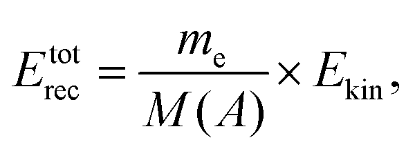 | (6) |
Which rotational and vibrational normal modes become recoil-excited depends crucially on the electron emission direction in the molecular frame. For example, in previous photoelectron recoil studies of the 1s photoemission, one assumptions in modeling has been that the orientation of the emitter molecules is isotropic.24,35,36 This follows from the fact that an atomic 1s orbital presents a spherically symmetric target to the ionizing radiation and therefore, if scattering of the outgoing photoelectron is neglected, orientation of the molecular axis becomes irrelevant in the photoemission process. The recoil lineshape is then obtained by equal-weight averaging over all emission directions in the molecular frame. However, for other that 1s photoemission, this assumption must be revisited when we consider the following cases.
Fig. 2 depicts the recoil lineshape calculated using the independent oscillator model27 at the photon energy of 7 keV, first using a low temperature of 30 K and no lifetime broadening for illustrative purposes (solid curve in the figure). The dashed curve corresponds to a room-temperature experiment (see Section 3.2) and also includes the 52 meV Lorentzian width.
 | ||
| Fig. 2 Simulated recoil lineshape for the S 2p photoemission from SF6 for hν = 7 keV at the temperature of 30 K and with no lifetime broadening (solid line) and at 300 K including the lifetime broadening (dotted line). The latter will be assigned to each Franck–Condon transition in describing experimental HAXPES spectra. | ||
At the 7 keV photon energy used for the calculation, the total recoil energy is 116.6 meV (as would be for the free sulfur atom), from which the translational recoil in the SF6 molecule is 25.7 meV. This translational recoil energy loss is seen as an overall shift of the recoil lineshape in Fig. 2 and, since there is no rotational recoil shift, is given by the position of the first vibrational peak. In the experiment, it would be seen as a shift of the photoelectron vibrational envelope towards lower kinetic energy (an apparent increase in binding energy). Secondly, no energy is received by the recoil-inactive rotations. Lastly, the lower-frequency T1u vibrations receive 16% of recoil energy and the higher-frequency ones 62% of the energy, giving rise to the vibrational progressions and the combination band in Fig. 2. The intensity-weighted average energy of the recoil lineshape corresponds to the total recoil energy of 116.6 meV and the width of the individual vibrational peaks in profiles is due to the thermal Doppler broadening which can be considered as a part of the recoil effect25,41–44 and therefore is inherently built into the model.27 The broadening is proportional to the temperature and to the electron kinetic energy.42
Anticipating the issues with photoelectron angular distribution with the next sample, it is worth discussing, how and if the angular anisotropy effects should be accounted for in the case of SF6. Firstly, the S 2p orbitals s–o components that are not MF-split are spherically symmetric, which means that the standard approach of the model,27 where the x-, y- and z-oscillators all receive equal share of the recoil momentum, is appropriate. Secondly, even if there were angular anisotropy in the molecular frame, there would still be no need for additional corrections. This is because the only two recoil-active vibrational modes are both triply degenerate (each creating three oscillators in the model), and the combined recoil energy received by these oscillators is independent of the emission-angle.
 | ||
| Fig. 3 Simulated recoil lineshapes for the S 2p photoemission from CS2 for hν = 7 keV, at T = 30 K and without lifetime broadening. Shape (a) corresponds to axial emission direction, (b) to perpendicular emission in respect to the molecular axis and (c) to isotropic emission. The latter would be assigned to each Franck–Condon transition in describing the experimental HAXPES spectrum, if the anisotropy effects can be neglected. | ||
A linear triatomic molecule is a simple enough case so that a numerical vibrational analysis is unnecessary and the recoil energy sharing is given just by momentum conservation and symmetry considerations. The total recoil energy is still the same as for SF6, 116.6 meV at 7-keV photon energy, but now, according to the mass ratio M(S)/M(CS2), 42% (49.1 meV) of the recoil energy goes into the molecular translation and the rest into the internal degrees of freedom. This translational recoil energy loss directly corresponds to the position of the first vibrational peak in the shape (a). The vibrational profile of (a) is dominated by the recoil-excited symmetric stretch excitations, for which the constant of 81.6 meV45 was used in the simulation. Weak asymmetric stretch excitations are also seen at 239 and 321 meV. The symmetric stretch excitations receive 50% and the asymmetric stretch 8% of the total recoil energy. Since in this case the recoil momentum is directed along the axis, there are no rotational excitations. Intensity-weighted average of the recoil shape (a) is at 116.6 meV (the total recoil energy).
The recoil shape (b) in Fig. 3 shows recoil excitations for the photoemission perpendicular to the molecular axis. Strong molecular rotational excitation occurs in this case, accompanied by weak bending-mode excitations. The stretching modes along the molecular axis are completely lacking in (b). Rotational excitations in perpendicular recoil replace the symmetric stretching vibrations in axial recoil, and also receive 50% of the recoil energy. Bending mode replaces the asymmetric stretching and receives 8% of the energy. Since individual rotational energy levels are not resolved in inner-shell photoelectron spectra, the rotational excitations are included in the model as an additional energy loss and broadening. The total recoil shift of the main peak in the shape (b) is 107.3 meV – a combination of translational and rotational recoil. The short vibrational series corresponds to the bending excitations with a constant of 49.2 meV.45
Lastly, the shape (c) represents isotropic emission where the axially excited modes receive 1/3 of the total recoil energy and the perpendicular modes 2/3. The shape is obtained by averaging over recoil shapes for different angles and therefore, as each angle has a different rotational recoil and the corresponding peak shifts, individual vibrational peaks can no longer be marked. In profile (c), there is an additional broadening – or a wash-out of the individual vibrational peaks – as their positions shift in the course of angle-averaging due to varying amount of rotational recoil.
The orientational distribution of molecules corresponding to all three 2p components detected in the spectrum was obtained in Section 2.1. Knowing these distributions (Fig. 1(b)) allows us to refine the recoil lineshapes of Fig. 3 using the appropriate weight functions. The results are shown in Fig. 4. The top graph shows the recoil lineshapes for S 2p photoemission of CS2 at hν = 7 keV, T = 30 K and without lifetime broadening, angle-averaged over all emission directions. Even after averaging, the shapes are distinctly different. The shape of 2p3/2,3/2 has the largest share of perpendicular emission and therefore the largest rotational shift. The mostly axial emission of the 2p3/2,1/2 component, on the other hand, creates the least energy shift but the strongest vibratonal excitations.
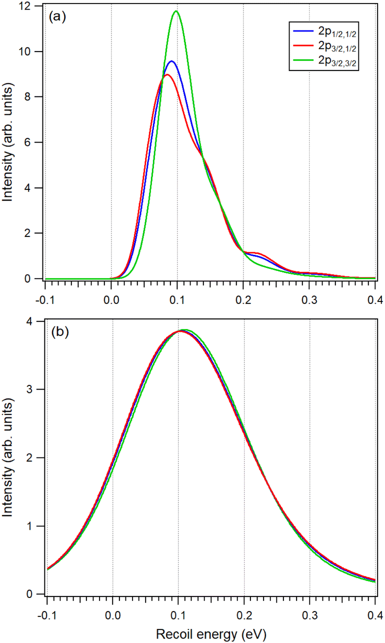 | ||
| Fig. 4 Simulated recoil lineshapes of the S 2p photoemission from CS2 at hν = 7 keV for the three s–o and MF split components. The shapes in panel (a) are obtained for T = 30 K without lifetime broadening and Franck–Condon vibrational excitations. Panel (b) shows the same distributions but for T = 300 K and including the lifetime broadening of 52 meV. Each Franck–Condon transition in the experimental HAXPES spectrum will be assigned one of the lineshapes in panel (b), according to the 2p component in question. | ||
Our analysis so far has demonstrated that, in the case of the joint s–o and MF effects on the inner-shell orbitals, the orientational anisotropy effects in the photoelectron recoil are relevant and should be taken into account. However, as the bottom graph of Fig. 4 demonstrates, the actual differences expected in the present experiment are quite minor. The graph shows the same recoil shapes, but now generated for the 300 K temperature and including the lifetime broadening. The translational and rotational Doppler broadenings increase from 50 (at 30 K) to 159 meV.
3 Experiment
3.1 Instrumental
The HAXPES experiment was performed at the SOLEIL Synchrotron, France, on the GALAXIES beamline equipped with an end station dedicated to hard and tender X-ray photoelectron spectroscopy.46,47 Linearly polarized light is provided by a U20 undulator and monochromatized by a Si(111) double crystal monochromator. At some energies it was necessary to reduce the photon flux at the sample in order to avoid nonlinearity effects associated with the readout of the chargecoupled device (CCD) detector of the Scienta spectrometer. This was achieved by introducing Al foil filters of 6 and 12 μm thickness into the beam. The samples and the calibration gas argon were introduced into a differentially pumped gas cell. The photoelectron spectra were recorded by a large acceptance angle EW4000 Scienta hemispherical analyzer, optimized for high kinetic-energy measurements. The spectrometer was mounted with the lens axis colinear with the polarization vector of the X-rays. In this experiment, the spectrometer was operated at 100-eV pass energy with the entrance slit of 0.5 mm (except for CS2 at 5 keV, where the 0.3 mm slit was used).The SF6 S 2p near-threshold photoelectron spectrum was recorded at the U56-2 PGM-1 beamline of the synchrotron radiation facility BESSY II in Helmholtz-Zentrum Berlin (HZB), Germany, using a Scienta R4000 photoelectron analyzer. The set-up is described in detail in ref. 48. For the present experiment, the pass energy of the analyzer was set to 20 eV and the entrance slit width to 0.3 mm, leading to a nominal electron energy resolution of 15 meV. A 400 l mm−1 plane grating of the monochromator was used in conjunction with a 50 μm exit slit. The spectrum presented here was recorded at a photon energy of 250 eV with a photon bandwidth of 45 meV and, to our knowledge, is the first published high-resolution S 2p photoelectron spectrum of SF6.
The near-threshold data for the S 2p photoemission from CS2 was obtained from literature, from the analysis of Wang et al.13
3.2 Measurements
 | ||
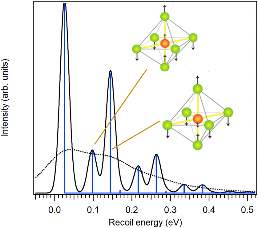
| Fig. 5 Sulfur 2p near-threshold photoelectron spectra from SF6 (a) and CS2 (b). Vertical bars mark the positions and heights of fitted peaks, with coulours differentiating the s–o and MF split components. Blue: 2p1/2,1/2, red: 2p3/2,1/2 and green 2p3/2,3/2. Spectrum (b) and its fitting results are reproduced from ref. 13. The inset graphics illustrate the Franck–Condon-excited vibrational modes. | ||
Carbon disulfide, CS2, is a linear molecule that belongs to the D∞h point group, where the degeneracy of the atomic p orbitals is partially removed. Thus, in addition to the s–o splitting as seen in the spectrum (a), spectrum (b) of Fig. 5 also exhibits a notably weaker MF splitting of the 2p3/2 peak.
In the curve fitting analysis of Wang et al.,13 reproduced here, the MF-splitting is shown in the spectrum (b) as the separation of green and red bars that mark the vibrational progressions belonging to the 2p3/2,3/2 and 2p3/2,1/2 MF-split components, respectively. The spectra were analyzed using a single harmonic vibrational progression obtaining the vibrational constant of 198 meV that corresponds to the asymmetric stretching mode.13 The MF-splitting was determined to be 128 meV and the lifetime broadening of the S 2p core-hole state was 59.6 meV.13
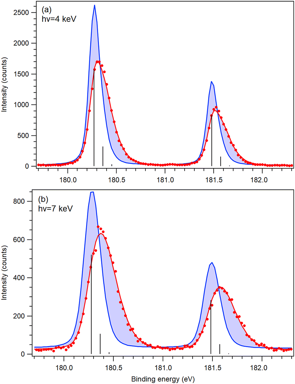 | ||
| Fig. 6 Least-squares fits (thick red curves) of the recoil lineshape to experimental S 2p photoelectron spectra of SF6 (full circles) measured at (a) 4 keV and (b) 7 keV photon energy. Vertical bars denote the positions of the individual Franck–Condon-excited vibrational peaks before any recoil shifts. Thick blue curves show, for reference, a simulated spectrum without the recoil effects and the change in the spectrum due to recoil is highlighted by shading. | ||
 | ||
| Fig. 7 Least-squares fits (thick red lines) of recoil lineshapes to experimental S 2p photoelectron spectra of CS2 (full circles) measured at (a) 5 keV and (b) 7 keV photon energy. Thin green-red-blue curves denote the individual s–o and MF split components of the fit. For reference, the vertical bars denote the positions of the individual Franck–Condon-excited vibrational peaks before recoil effects, thick blue curves show the simulated no-recoil spectrum and the change in the spectrum due to recoil is highlighted by shading. | ||
As in the case of SF6, the Gaussian instrumental broadening was given as a free parameter and we obtained it as 122(15) (hν = 5 keV) and 245(35) meV (hν = 7 keV).
3.3 Trends and comparison with theory
The strength of the recoil excitations of the individual vibrational levels is included in the recoil shape, used in the fitting of the HAXPES spectra (Fig. 6 and 7) instead of the usual Voigt profile. That being the case, the agreement between the model prediction and the experiment is evaluated by the overall goodness of the fit rather than the individual peak intensities. All least-squares fits of the spectra represent the experimental spectra well without noticeable systematic residual deviations, with the reduced χ2 of 1.27 (hν = 4 keV) and 1.16 (hν = 7 keV) for SF6, and 0.91 (hν = 5 keV) and 0.82 (hν = 7 keV) for CS2, obtained with a very limited number of free parameters.The overall effect of the photoelectron recoil results in very significant changes – peak shifts and broadenings – in the photoelectron spectra, as indicated by the shaded areas in Fig. 6 and 7. However, the vibrational structure is not resolved, which makes a stringent test of the modelled recoil ineshapes problematic. A major limiting factor in this case is the Doppler broadening, since the sample was at there room temperature. In CS2, for example, it contributes 159 meV to the total Gaussian broadening at hν = 7 keV.
Apart from the reduced χ2 goodness test of the fit, a useful free parameter to examine is the width of the Gaussian profile that convolutes the recoil lineshape and represents the instrumental (photon bandwidth and electron energy resolution) contributions. Another Gaussian broadening is due to the Doppler effect, which is already built into the recoil lineshape. The least-squares result for the instrumental broadenings can be compared with the values obtained from argon 2p calibration and reference spectra, and also with the nominal instrumental resolution data, as shown in Fig. 8. One can see that (i) the argon spectra confirm the nominal instrumental resolution and that (ii) the recoil-shape fit of SF6 (full blue circles) yields a Gaussian broadening that very well represents the instrumental contribution. One indication of the importance of the inclusion of recoil effects is given, when the spectra are analyzed by Voigt lineshapes instead of the recoil ones, therefore removing all recoil effects. The open blue circles in Fig. 8 represent a least-squares fitting with Voigt lineshapes. The least-squares procedure compensates for the neglected recoil excitations by additional shifts and an extra broadening of the Voigt peaks. Indeed, the obtained Gaussian widths are now much larger. Even after removing the Doppler contributions from the Voigt Gaussian component (these values are shown in Fig. 8), a clear discrepancy with the nominal instrumental width indicates the deficiency of this non-recoil analysis.
 | ||
| Fig. 8 Instrumental broadenings (full-width at half-maximum) in the HAXPES spectra, as determined by least-squares fitting and compared to the nominal values of the instrumental resolution. Multiple values for Ar 2p result from different series of measurements. The error bars reflect only the statistical error in the least-squares fitting. | ||
Turning to CS2, the Gaussian broadening obtained from the recoil-shape fit (full red circles in Fig. 8) also agrees very well with the nominal instrumental contribution at hν = 5 keV and hν = 4 keV and becomes too large when the recoil effects are neglected in the lineshape. Note that the datapoints here include a value at hν = 4 keV, not shown in Fig. 7 because of its inferior statistics. At hν = 7 keV, there is a discrepancy – even with the recoil-shape fit, the obtained Gaussian broadening is too large, indicating an unaccounted-for contribution or a deficient fitting model. Here, too, removal of the recoil effects (open red circles) results in extra Gaussian broadening.
For CS2, the vibrationally unresolved recoil lineshapes (Fig. 4(b)) have the FWHM of about 220 meV at hν = 7 keV, including the lifetime broadening. Deficiencies in the recoil model affecting this width (or a significant underestimation of the actual sample gas temperature) could be compensated in the fitting by an overly large Gaussian width. However, the experimental spectrum is a result of many hours of measurement with some variations in photon flux and gas pressure and drifts of the source potential were observed over this period (as usual). Although re-alignment of individual scans was performed as accurately as possible, we consider that the most likely explanation for this additional broadening is an imperfectly compensated source potential drift over a long measurement. This explanation is supported by the fact that an additional broadening is present also in the hν = 7 keV C 1s photoelectron spectra, taken interleavingly with the S 2p scans: 318 meV instead of the 159 meV.
Let us now turn to the question, whether the theoretical results of this paper – effects of the orientational anisotropy of the MF-split components of the S 2p photoelectron spectra on the recoil excitations – can be fully tested with the state-of-art HAXPES gas-phase photoelectron spectra. In short: no. Replacing the modelled recoil shapes with the ones that assume isotropic orientations for all MF-split components does not result in a statistically meaningful increase in the χ2 value. Would the effect be verifiable with further experimental advances? Although the Franck–Condon structure cannot be eliminated, a major factor is the Doppler broadening that is proportional to  .27 Firstly, carrying out the measurement at the liquid nitrogen temperature would significantly reduce this contribution. Secondly, the instrumental broadening could be reduced and the counting statistics improved at brighter X-ray sources. Fig. 9 explores the potential impact of such improvements by comparing two modelled S 2p photoelectron spectra. The dotted curves show the modelled total S 2p photoelectron spectra of CS2 using recoil model with (red) and without (green) anisotropy effects. Although these curves are still very similar, the black dashed line highlights their differences. With as much as 6% discrepancies in some regions of the spectra, when using the predicted vs. isotropic molecular orientations, the effect should be experimentally verifiable with sufficient statistics.
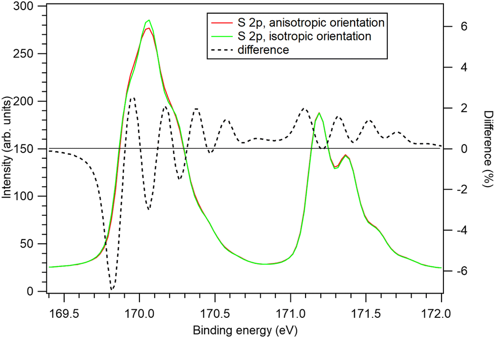 | ||
| Fig. 9 Generated S 2p photoelectron spectra for hν = 7 keV, using the fitted structure of Fig. 8(b), but reducing the temperature to 70 K and instrumental broadening to 60 meV (equal to the lifetime broadening). Red: using the theoretically predicted molecular orientation distributions for and green: using isotropic distributions for all components. The black dashed line is the difference between the first and the second spectrum. | ||
Alternatively, in electron–ion coincident spectroscopy where one can determine the molecular axis using the ion momenta from the Coulomb explosion, one can uniquely determine the emission angle in the molecular frame for each electron and therefore perform a fully orientationally resolved measurement, assuming that an electron resolution comparable to that of high-resolution photoelectron spectrum can be achieved.
4 Conclusions
Molecular field splitting lifts the degeneracy of atomic inner-shell orbitals with l > 0, which has a range of consequences in molecular inner-shell photoemission. Such a splitting occurs for sulfur 2p orbitals in CS2, but is absent in SF6. Even though retaining the atomic nature of the wavefunctions, the spherical harmonic representation of the MF- and s–o split components shows that they are anisotropic in the molecular frame. From this, we have derived in general form the orientation distribution of linear molecules, emitting photoelectrons in the direction of the linear polarization vector of the incident X-ray beam, for each MF- and s–o split component of the 2p wavefunction. Applying this result to the recoil model, we then demonstrated, how this anisotropy affects the recoil excitations to different vibrational and rotational degrees of freedom. For example, axial (vibrational) recoil dominated for the CS2 molecules emitting the 2p3/2,1/2 component, while in the case of the 2p3/2,3/2 component, the transverse (rotational and bending) excitations were dominant. As a result, the total recoil lineshape, produced by the independent oscillator model, is different for each MF- and s–o split component. This demonstrates that, in principle, the strong recoil effects in HAXPES regime carry orientational information about the photoemitter, although these lineshape effects are rather subtle. As a result, the state-of-art gas-phase HAXPES measurements that were performed to test the theoretical modeling are not yet able to extract these effects, although they confirm the applicability of the independent oscillator recoil model in general. Further developments in synchrotron-radiation HAXPES techniques could bring a direct experimental confirmation of the recoil anisotropy effects. Also, HAXPES experiments in the fixed-in-space molecular frame by coincidence spectroscopy would provide a stringent test of the anisotropy effects in recoil.Data availability
Orientational anisotropy due to molecular field splitting in sulfur 2p photoemission from CS2 and SF6 – theoretical treatment and application to photoelectron recoil. Data for this article, including the photoelectron spectra in both raw (individual scans) and processed (summed, calibrated) are available at SeaFile depository of the University of Turku at https://seafile.utu.fi/d/b69303456f85443e8e06/. In case access password is required, it is provided by the authors.Conflicts of interest
The authors declare that they have no known competing financial interests or personal relationships that could have appeared to influence the work reported in this paper.Acknowledgements
We thank the staff of the GALAXIES beamline for their invaluable support during the measurements. EK acknowledges the Research Council of Finland, and MB the Estonian Research Council grant (MOBTP1013) for the financial support. We acknowledge Helmholtz-Zentrum Berlin for the allocation of synchrotron radiation beamtime at Bessy II. We also thank Tiberiu Arion and Cosmin Lupulescu for their contributions to the measurement of the low photon energy spectrum of SF6 at Bessy II, Wolfgang Eberhardt for his support of this activity and Renaud Guillemin and Tatiana Marchenko for their contribution to the experiment at the GALAXIES beamline.Notes and references
- G. Greczynski and L. Hultman, Prog. Mater. Sci., 2020, 107, 100591 CrossRef CAS
.
- T. X. Carroll, K. J. Børve, L. J. Sæthre, J. D. Bozek, E. Kukk, J. A. Hahne and T. D. Thomas, J. Chem. Phys., 2002, 116, 10221 CrossRef CAS
- W. Eberhardt, S. Bernstorff, H. W. Jochims, S. B. Whitfield and B. Crasemann, Phys. Rev. A: At., Mol., Opt. Phys., 1988, 38, 3808–3811 CrossRef CAS PubMed
- U. Hergenhahn, J. Phys. B: At., Mol. Opt. Phys., 2004, 37, R89 CrossRef CAS
- E. U. Condon, Phys. Rev., 1928, 32, 858–872 CrossRef CAS
- L. Cederbaum and W. Domcke, J. Chem. Phys., 1974, 60, 2878–2889 CrossRef CAS
- L. Zhang, M. Wei, G. Ge and W. Hua, Phys. Rev. A: At., Mol., Opt. Phys., 2024, 109, 032815 CrossRef CAS
- S. Suga and A. Sekiyama, Eur. Phys. J.-Spec. Top., 2009, 169, 227–235 CrossRef
-
S. Suga and A. Sekiyama, Photoelectron Spectroscopy, Springer Berlin Heidelberg, Berlin, Heidelberg, 2014, vol. 176 Search PubMed
- M. Kircher, J. Rist, F. Trinter, S. Grundmann, M. Waitz, N. Melzer, I. Vela-Perez, T. Mletzko, A. Pier, N. Strenger, J. Siebert, R. Janssen, V. Honkimäki, J. Drnec, P. Demekhin, L. Schmidt, M. Schöffler, T. Jahnke and R. Dörner, Phys. Rev. Lett., 2019, 123, 193001 CrossRef CAS PubMed
- M. N. Piancastelli, T. Marchenko, R. Guillemin, L. Journel, O. Travnikova, I. Ismail and M. Simon, Rep. Prog. Phys., 2020, 83, 016401 CrossRef CAS PubMed
- E. Kukk, R. Püttner and M. Simon, Phys. Chem. Chem. Phys., 2022, 24, 10465–10474 RSC
- H. Wang, M. Bässler, I. Hjelte, F. Burmeister and L. Karlsson, J. Phys. B: At., Mol. Opt. Phys., 2001, 34, 1745–1755 CrossRef CAS
- C. P. Flynn, Phys. Rev. Lett., 1976, 37, 1445–1448 CrossRef CAS
- T. Fujikawa, R. Suzuki and L. Kövér, J. Electron Spectrosc. Relat. Phenom., 2006, 151, 170–177 CrossRef CAS
- W. Domcke and L. Cederbaum, J. Electron Spectrosc. Relat. Phenom., 1978, 13, 161–173 CrossRef CAS
- E. Kukk, K. Ueda, U. Hergenhahn, X.-J. Liu, G. Prümper, H. Yoshida, Y. Tamenori, C. Makochekanwa, T. Tanaka, M. Kitajima and H. Tanaka, Phys. Rev. Lett., 2005, 95, 133001-1 CrossRef PubMed
- Y. Takata, Y. Kayanuma, M. Yabashi, K. Tamasaku, Y. Nishino, D. Miwa, Y. Harada, K. Horiba, S. Shin, S. Tanaka, E. Ikenaga, K. Kobayashi, Y. Senba, H. Ohashi and T. Ishikawa, Phys. Rev. B: Condens. Matter Mater. Phys., 2007, 75, 233404 CrossRef
- E. Kukk, T. Thomas and K. Ueda, J. Electron Spectrosc. Relat. Phenom., 2011, 183, 53–58 CrossRef CAS
- M. Ehara, H. Nakatsuji, M. Matsumoto, T. Hatamoto, X.-J. Liu, T. Lischke, G. Prümper, T. Tanaka, C. Makochekanwa, M. Hoshino, H. Tanaka, J. R. Harries, Y. Tamenori and K. Ueda, J. Chem. Phys., 2006, 124, 124311 CrossRef CAS PubMed
-
Y. Kayanuma, in Hard X-ray Photoelectron Spectroscopy (HAXPES), ed. J. Woicik, Springer International Publishing, Cham, 2016, vol. 59, pp. 175–195 Search PubMed
- Y. Krivosenko and A. Pavlychev, Chem. Phys. Lett., 2013, 575, 107–111 CrossRef CAS
- Y. Krivosenko and A. Pavlychev, Chem. Phys. Lett., 2016, 233–236 CrossRef CAS
- E. Kukk, T. Thomas, D. Céolin, S. Granroth, O. Travnikova, M. Berholts, T. Marchenko, R. Guillemin, L. Journel, I. Ismail, R. Püttner, M. Piancastelli, K. Ueda and M. Simon, Phys. Rev. Lett., 2018, 121, 073002 CrossRef CAS PubMed
- F. Gelmukhanov, H. Ågren and P. Sałek, Phys. Rev. A: At., Mol., Opt. Phys., 1998, 57, 2511–2526 CrossRef CAS
- T. D. Thomas and K. Ueda, J. Electron Spectrosc. Relat. Phenom., 2014, 195, 101–108 CrossRef CAS
- E. Kukk, D. Céolin, O. Travnikova, R. Püttner, M.-N. Piancastelli, R. Guillemin, L. Journel, T. Marchenko, I. Ismail, J. Martins, J.-P. Rueff and M. Simon, New J. Phys., 2021, 063077 CrossRef CAS
- T. D. Thomas, R. Püttner, H. Fukuzawa, G. Prümper, K. Ueda, E. Kukk, R. Sankari, J. Harries, Y. Tamenori, T. Tanaka, M. Hoshino and H. Tanaka, J. Chem. Phys., 2007, 127, 244309 CrossRef PubMed
- T. D. Thomas, L. J. Saethre, K. J. Børve, J. D. Bozek, M. Huttula and E. Kukk, J. Phys. Chem. A, 2004, 108, 4983–4990 CrossRef CAS
- K. J. Børve, Chem. Phys. Lett., 1996, 262, 801–806 CrossRef
- J. L. Dehmer and D. Dill, J. Chem. Phys., 1976, 65, 5327–5334 CrossRef CAS
- D. Dill, J. R. Swanson, S. Wallace and J. L. Dehmer, Phys. Rev. Lett., 1980, 45, 1393–1396 CrossRef CAS
- M. Kircher, J. Rist, F. Trinter, S. Grundmann, M. Waitz, N. Melzer, I. Vela-Pérez, T. Mletzko, A. Pier, N. Strenger, J. Siebert, R. Janssen, L. Schmidt, A. Artemyev, M. Schöffler, T. Jahnke, R. Dörner and P. Demekhin, Phys. Rev. Lett., 2019, 123, 243201 CrossRef CAS PubMed
- F. Gel’mukhanov, H. Ågren, S. Svensson, H. Aksela and S. Aksela, Phys. Rev. A: At., Mol., Opt. Phys., 1996, 53, 1379–1387 CrossRef PubMed
- T. D. Thomas, E. Kukk, R. Sankari, H. Fukuzawa, G. Prümper, K. Ueda, R. Püttner, J. Harries, Y. Tamenori, T. Tanaka, M. Hoshino and H. Tanaka, J. Chem. Phys., 2008, 128, 144311 CrossRef PubMed
- E. Kukk, K. Ueda and C. Miron, J. Electron Spectrosc. Relat. Phenom., 2012, 185, 278–284 CrossRef CAS
- G. M. J. Barca, C. Bertoni, L. Carrington, D. Datta, N. De Silva, J. E. Deustua, D. G. Fedorov, J. R. Gour, A. O. Gunina, E. Guidez, T. Harville, S. Irle, J. Ivanic, K. Kowalski, S. S. Leang, H. Li, W. Li, J. J. Lutz, I. Magoulas, J. Mato, V. Mironov, H. Nakata, B. Q. Pham, P. Piecuch, D. Poole, S. R. Pruitt, A. P. Rendell, L. B. Roskop, K. Ruedenberg, T. Sattasathuchana, M. W. Schmidt, J. Shen, L. Slipchenko, M. Sosonkina, V. Sundriyal, A. Tiwari, J. L. Galvez Vallejo, B. Westheimer, M. Wloch, P. Xu, F. Zahariev and M. S. Gordon, J. Chem. Phys., 2020, 152, 154102 CrossRef CAS PubMed
- A. D. Becke, J. Chem. Phys., 1992, 96, 2155–2160 CrossRef CAS
- T. H. Dunning Jr, J. Chem. Phys., 1989, 90, 1007–1023 CrossRef
- M. W. Chase Jr., J. Phys. Chem. Ref. Data, 1985, 14 Search PubMed
- Y.-P. Sun, C.-K. Wang and F. Gelmukhanov, Phys. Rev. A: At., Mol., Opt. Phys., 2010, 82, 052506 CrossRef
- T. Thomas, E. Kukk, K. Ueda, T. Ouchi, K. Sakai, T. Carroll, C. Nicolas, O. Travnikova and C. Miron, Phys. Rev. Lett., 2011, 106, 193009 CrossRef CAS PubMed
- M. Simon, R. Püttner, T. Marchenko, R. Guillemin, R. K. Kushawaha, L. Journel, G. Goldsztejn, M. N. Piancastelli, J. M. Ablett, J.-P. Rueff and D. Céolin, Nat. Commun., 2014, 5, 4069 CrossRef CAS PubMed
- D. Céolin, J.-C. Liu, V. Vaz da Cruz, H. Ågren, L. Journel, R. Guillemin, T. Marchenko, R. K. Kushawaha, M. N. Piancastelli, R. Püttner, M. Simon and F. Gelmukhanov, Proc. Natl. Acad. Sci. U. S. A., 2019, 116, 4877–4882 CrossRef PubMed
- T. Shimanouchi, Tables of molecular vibrational frequencies, consolidated volume i, National Bureau of Standards Technical Report NBS NSRDS 39, 1972.
- D. Céolin, J. Ablett, D. Prieur, T. Moreno, J.-P. Rueff, T. Marchenko, L. Journel, R. Guillemin, B. Pilette, T. Marin and M. Simon, J. Electron Spectrosc. Relat. Phenom., 2013, 190, 188–192 CrossRef
- J.-P. Rueff, J. M. Ablett, D. Céolin, D. Prieur, T. Moreno, V. Balédent, B. Lassalle-Kaiser, J. E. Rault, M. Simon and A. Shukla, J. Synchrotron Radiat., 2015, 22, 175–179 CrossRef CAS PubMed
- C. Lupulescu, T. Arion, U. Hergenhahn, R. Ovsyannikov, M. Förstel, G. Gavrila and W. Eberhardt, J. Electron Spectrosc. Relat. Phenom., 2013, 191, 104–111 CrossRef CAS
- E. Hudson, D. A. Shirley, M. Domke, G. Remmers, A. Puschmann, T. Mandel, C. Xue and G. Kaindl, Phys. Rev. A: At., Mol., Opt. Phys., 1993, 47, 361–373 CrossRef CAS PubMed
Footnote |
| † Electronic supplementary information (ESI) available. See DOI: https://doi.org/10.1039/d4cp01463d |
| This journal is © the Owner Societies 2024 |