Solvation dynamics on the diffusion timescale elucidated using energy-represented dynamics theory†
Received
18th January 2024
, Accepted 1st April 2024
First published on 16th April 2024
Abstract
Photoexcitation of a solute alters the solute–solvent interaction, resulting in the nonequilibrium relaxation of the solvation structure, often called a dynamic Stokes shift or solvation dynamics. Thanks to the local nature of the solute–solvent interaction, the characteristics of the local solvent environment dissolving the solute can be captured by the observation of this process. Recently, we derived the energy-represented Smoluchowski–Vlasov (ERSV) equation, a diffusion equation for molecular liquids, which can be used to analyze the solvation dynamics on the diffusion timescale. This equation expresses the time development for the solvent distribution on the solute–solvent pair interaction energy (energy coordinate). Since the energy coordinate can effectively treat the solvent flexibility in addition to the position and orientation, the ERSV equation can be utilized in various solvent systems. Here, we apply the ERSV equation to the solvation dynamics of 6-propionyl-2-dimethylamino naphthalene (Prodan) in water and different alcohol solvents (methanol, ethanol, and 1-propanol) for clarifying the differences of the relaxation processes among these solvents. Prodan is a solvent-sensitive fluorescent probe and is thus widely utilized for investigating heterogeneous environments. On the long timescale, the ERSV equation satisfactorily reproduces the relaxation time correlation functions obtained from the molecular dynamics (MD) simulations for these solvents. We reveal that the relaxation time coefficient on the diffusion timescale linearly correlates with the inverse of the translational diffusion coefficients for the alcohol solvents because of the Prodan-solvent energy distributions among the alcohols. In the case of water, the time coefficient deviates from the linear relationship for the alcohols due to the difference in the extent of importance of the collective motion between the water and alcohol solvents.
1 Introduction
Solute–solvent interaction is vital for the mass transport as well as the chemical reaction of a solute. The friction associated with the solute motion is affected by such an interaction in addition to the solvent diffusivity.1–3 The motion of the solvent molecules around the solute is also different from the simple diffusion in the bulk phase due to the inhomogeneous environment produced by a solute.4 Photoexcitation phenomena give us useful information on the solute–solvent interaction through spectroscopy techniques. The local solvent environments can be elucidated by the fluorescence spectra of solvent-sensitive probes. The spectra are often characterized using physicochemical concepts such as Stokes shifts and polarity.5,6 Furthermore, the solvent response to the change in the electronic structure of a solute by the photoexcitation, referred to as solvation dynamics or dynamic Stokes shift, reflects the dynamic properties of solvents.4,7,8 The solvation dynamics can be utilized for investigating the heterogeneous environments such as the ionic liquids,9–11 biomolecular solutions12,13 and biological membranes.14–16
Theoretical and computational methods are useful for obtaining atomistic information about the photoexcitation dynamics in solutions which is difficult to be accessed from the experiments only. Molecular dynamics (MD) simulation is a representative method to obtain such information.17,18 The solvation dynamics of small solute molecules such as coumarin has been extensively studied by means of MD simulations so far.8,19–21 The recent advances in computers enables us to investigate the solvation dynamics of macromolecules such as deoxyribonucleic acids (DNA)22 and proteins23 in aqueous solutions. Ab initio MD (AIMD) simulation24 is also a powerful tool for realistically describing solvation dynamics.25,26 For instance, the application of this method to the solvation dynamics of N-methyl-6-oxyquinolinium betaine in water revealed that the dominant mode for the solvent motion varies depending on the timescale and that the collective solvent rearrangement plays an important role on a picosecond timescale.26 However, the accurate computation of the time correlation functions on the long timescale often suffers from the insufficient sampling.
The dynamics theories based on the integral equation theory of molecular liquids with the interaction-site representation27–29 have been also widely used to investigate the solvation dynamics of the various solutes in molecular liquids.30–40 The governing equations have a mathematically closed form for both the static and dynamic properties of solutions, and hence information on the dynamics can be obtained by solving the equations in an algebraic manner, meaning that the obtained results are free from the sampling problem.41–45 The application of these theories to the solvation dynamics is possible with the aid of a modified linear response theory32,34 or time-dependent density functional theory (TD-DFT) of liquids.4,45–47 Due to the orientational average of solvent molecules introduced for avoiding the explicit treatment of the orientational degrees of freedom, however, theories with the interaction-site representation are applicable only to the simple polyatomic solvents. In addition, the rigidity of the molecules is assumed in these theories. Note that the flexibility of molecules is known to have an impact on the dynamic behavior of solutions.48,49
Recently, we have derived an alternative expression for the molecular diffusion based on the energy representation (ER) which is amenable to MD simulations.50 In this theory, the configuration of a solvent molecule is projected onto the solute–solvent interaction energy, namely the energy coordinate.51–53 It should be noted that the intramolecular degree of freedom is naturally taken into account using the energy coordinate. This dimensionality reduction also enables us to construct the one-dimensional free-energy functional for describing the solvation thermodynamics in complex solutions including polymer solutions54 and lipid membrane systems55,56 by means of MD simulations. By applying the Zwanzig–Mori projection operator method to the solvent distribution on the energy coordinate, the energy-represented generalized Langevin equation (ERGLE) can be derived in an exact way.50 The systematic approximations about the dynamics such as the overdamped limit give the energy-represented Smoluchowski–Vlasov (ERSV) equation, a diffusion equation of solution that describes the self-diffusion, drift motion, and collective motion of solvents on the energy coordinate. Once we calculate the static correlation functions and diffusion coefficient of solvents involved in the ERSV equation, the time development of the solvent distribution functions can be obtained by solving this equation. Since the sampling of the information on the dynamics is not required in this treatment, the analysis of the long-timescale dynamics is realized without the sampling problem. It is confirmed that the ERSV equation reproduces the relaxation time coefficient on the diffusion timescale for the solvation dynamics of benzonitrile in water. Furthermore, we revealed the importance of the collective diffusion on the solvent relaxation on the intermediate timescale.
In the present study, we apply the ERSV equation to the solvation dynamics of 6-propionyl-2-dimethylamino naphthalene (Prodan) in water and alcohol solvents (methanol, ethanol, and 1-propanol) for clarifying the differences between the relaxation processes among these solvents. Prodan is a solvent-sensitive fluorescence probe that exhibits significant Stokes shifts, making it possible to analyze the local environments of the systems of interest.57–62 The excited states of Prodan are well characterized using quantum chemical calculations.63–66 Prodan is widely used for analyzing the membrane properties such as local polarity and gel phase transition.67–70 The time-resolved infrared (IR) spectroscopy analysis of the solvent-dependent feature of the excited state for Prodan probed that the S1(π–π*) state undergoing a solvent-driven charge redistribution from dimethylamine (DMA) to the carbonyl (C![[double bond, length as m-dash]](https://www.rsc.org/images/entities/char_e001.gif) O) group dynamically alters the solvation structure such as the patterns in hydrogen-bonding of Prodan with the surrounding solvent molecules, suggesting the importance of the atomistic description of the solvation dynamics.62 Very recently, the systematic analysis of the membrane properties at the interfacial region was proposed based on the fluorescence decays of Prodan in a series of solvent mixtures.71 The microscopic information on the solvation dynamics in various solvents could thus be useful to deepen our understanding of heterogeneous environments.
O) group dynamically alters the solvation structure such as the patterns in hydrogen-bonding of Prodan with the surrounding solvent molecules, suggesting the importance of the atomistic description of the solvation dynamics.62 Very recently, the systematic analysis of the membrane properties at the interfacial region was proposed based on the fluorescence decays of Prodan in a series of solvent mixtures.71 The microscopic information on the solvation dynamics in various solvents could thus be useful to deepen our understanding of heterogeneous environments.
We focus on the solvation dynamics of Prodan triggered by S1(π–π*) excitation described by means of the TD-DFT of electronic structures. The solvation time correlation function (STCF) for each solvent is calculated using the ERSV equation based on the MD simulations with Prodan in its ground state. Furthermore, we introduce a scheme for decomposing the diffusion coefficients in the energy representation into the contributions of the moieties in Prodan to unveil the difference between the relaxation processes depending on the solvent species.
2 Methods
2.1 Energy-represented Smoluchowski–Vlasov (ERSV) equation
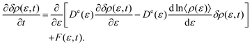
In this section, we briefly summarize the energy-represented dynamics theory and its application to the solvation dynamics.50 The energy representation means that the solvent configuration around a solute is projected onto the solute–solvent pair interaction energy, the energy coordinate. Then, the dynamic processes of solvents are represented as the time development of the solvent distribution on the energy coordinate in the theory. This treatment enables us to effectively treat the solvent position and orientation on one-dimensional space.
Let us consider a dilute solution containing a solute molecule in a single-component solvent. The formulation for multi-component solvents is available in ref. 50. Furthermore, we assume that the solute molecule is fixed in space. We define the full coordinate (position and orientation with the intramolecular degrees of freedom) of the ith solvent molecule as xi. The instantaneous solvent distribution on the energy coordinate (energy distribution), ρ(ε,t), is defined as
| |  | (1) |
where
u(·) is an energy function between the solute and solvent (defining potential). The fluctuation of
ρ(
ε,
t) is also defined as
| | | δρ(ε,t) = ρ(ε,t) − 〈ρ(ε)〉, | (2) |
where 〈⋯〉 represents the ensemble average at the equilibrium state. The Zwanzig–Mori projection operator method gives the energy-represented generalized Langevin equation (ERGLE), an exact partial differential equation of
δρ(
ε,
t). Imposing the overdamped limit on the ERGLE, one can derive the energy-represented Smoluchowski–Vlasov (ERSV) equation given by
| |  | (3) |
Here,
De(
ε) and
F(
ε,
t) mean the energy-represented diffusion coefficient and fluctuating force, respectively.
c(
ε,
η) is the direct correlation function that describes the relationship between the solvent molecules whose values of the defining potential are
ε and
η. The approximate expression of
De(
ε) is given by
where
D and
fGi are the translational diffusion coefficient of the solvent in the bulk and the force acting on the center of mass (CoM) of the
ith solvent molecule conditioned by the value of the defining potential, respectively. 〈⋯〉
ε means the ensemble average conditioned by the energy coordinate
ε defined as
| |  | (5) |
Thanks to the additivity of the solute–solvent interaction, fGi can be decomposed into the forces acting on the moieties (m) of the solute molecule, fmi, as
| |  | (6) |
Thus,
De(
ε) can be rewritten as
| |  | (7) |
| | | De,m(ε) = D〈fmi·fGi〉ε. | (8) |
Note that
De,m(
ε) can be regarded as the contribution of moiety
m to
De(
ε).
Each term in the ERSV equation (eqn (3)) has a clear physical meaning. The first term in the square bracket of eqn (3) describes the simple diffusion of solvents due to the gradient of the solvent distribution. Since −ln![[thin space (1/6-em)]](https://www.rsc.org/images/entities/char_2009.gif) 〈ρ(ε)〉 multiplied by the inverse temperature is the free energy profile on the energy coordinate, the drift motion caused by the free energy gradient is expressed using the second term. The third term describes the collective diffusion through the direct correlation function, c(ε,η). If the collective term is neglected in the ERSV equation (eqn (3)), one can obtain the energy-represented Smoluchowski equation (ERS) describing the single-particle diffusion process as
〈ρ(ε)〉 multiplied by the inverse temperature is the free energy profile on the energy coordinate, the drift motion caused by the free energy gradient is expressed using the second term. The third term describes the collective diffusion through the direct correlation function, c(ε,η). If the collective term is neglected in the ERSV equation (eqn (3)), one can obtain the energy-represented Smoluchowski equation (ERS) describing the single-particle diffusion process as
| |  | (9) |
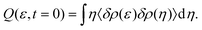
The solvation dynamics triggered by the sudden change of a solute molecule can be described based on the ERSV equation and linear response theory.72,73 Let us consider a nonequilibrium process in which the solute–solvent pair interaction energy is changed from ug(xi) to uex(xi) due to the photoexcitation of a solute at t = 0. If we assume that the intramolecular energy of the solute is unchanged during the relaxation process, the solvation time correlation function (STCF), S(t), can be expressed as
| |  | (10) |
where 〈⋯〉
ne is the nonequilibrium ensemble average and
| |  | (11) |
Next, we introduce a scheme for describing the solvation dynamics. The solvation dynamics is characterized with the solvation time correlation function (STCF), S(t). Based on the linear response theory, S(t) can be expressed as
| |  | (12) |
Here, 〈⋯〉 is the ensemble average at the ground state and δΔE(t) is the fluctuation of ΔE(t) defined as δΔE(t) = ΔE(t) − 〈ΔE〉. If the defining potential is the difference of the solute–solvent pair interaction energies between the excited and ground states as u(xi) = uex(xi) − ug(xi), δΔE(t) and its autocorrelation function can be written as
| |  | (13) |
| |  | (14) |
where we have introduced a new function
Q(
ε,
t) defined as
| |  | (15) |
Substituting
eqn (14) into
eqn (12) yields
| |  | (16) |
By using
eqn (3), one can obtain the ERSV equation for
Q(
ε,
t) as
| |  | (17) |
The ERS equation for
Q(
ε,
t) can be also derived from
eqn (9) as
| |  | (18) |
The STCF can be computed by solving the ERSV or ERS equation under the following initial conditions.
| |  | (19) |
2.2 Computational details
2.2.1 System modeling.
The structure of Prodan (Fig. 1) was obtained by performing geometry optimization using CAM-B3LYP/cc-pVDZ level calculations74 at the ground state. Then, the S1(π → π*) excited state was computed using TD-DFT (CAM-B3LYP)/cc-pVDZ calculations. Charges from electrostatic potentials using a grid based method (CHelpG)75 was used for calculating the atomic point charges for both the ground and excited states (Table S1 and Fig. S1, ESI†). All the quantum chemical calculations were performed using Gaussian16.76
 |
| | Fig. 1 Structure of Prodan. The hydrogen, carbon, nitrogen and oxygen atoms are depicted in gray, green, blue and red, respectively. | |
We prepared four different solution systems consisting of one Prodan molecule and solvent molecules, water, methanol (MeOH), ethanol (EtOH), and 1-propanol (PrOH). The force field for Prodan, MeOH, EtOH, and PrOH was the CHARMM generalized force field (CGenFF)77 and the parameters were obtained using the CHARMM-GUI server,78 while the atomic charges on Prodan for the ground and excited states were evaluated using the quantum chemical calculations mentioned above. The CHARMM-compatible TIP3P model was used for water.79 The numbers of solvent molecules were 7200, 3100, 2210, and 1690 for water, methanol, ethanol, and 1-propanol systems, respectively. For all the systems, the initial configurations were prepared using Packmol80 with the cubic box whose volume is 603 Å3. We also prepared the pure solvent systems for calculating the diffusion coefficients of the solvents. The numbers of solvent molecules and the volume are the same as those for the corresponding solution systems.
2.2.2 Simulation setups.
For each solution system with Prodan in its ground state, we performed three types of NVT simulations: (i) equilibration, (ii) sampling of the system configurations and (iii) production simulations started from the configurations obtained from (ii). For equilibration (i), the MD simulations were performed for 1 ns. Then, we conducted the simulation (ii) for 1 ns to extract the configurations every 1 ps (the total number of the samples was 1000 for each system). After re-distributing the velocities of the sampled configurations so as to generate the Maxwell–Boltzmann distribution, we performed the simulations (iii) for 0.1 ns equilibration, followed by 1 ns production simulation for each trajectory. As for each pure-solvent system, we performed 0.4 ns production simulation after 1 ns simulation for equilibration.
For all the simulations, the equation of motion was integrated using the velocity Verlet algorithm81 with a time interval of 2 fs. The temperature was set at 300 K using the Bussi thermostat.82 The Prodan molecule was fixed in space by making the velocities of its atoms zero. The Lennard-Jones (LJ) interaction was truncated by applying the switching function, with the switching range of 10–12 Å. The smooth particle mesh Ewald (SPME) method83,84 was used to calculate the electrostatic potential. Water molecules were kept rigid using the SETTLE algorithm85 and the bonds involving the hydrogen atoms were fixed using the SHAKE/RATTLE algorithm.86,87 All the simulations were performed with GENESIS 2.0.88–90 All the analyses were performed using in-house Fortran90/95 programs combined with the visual molecular dynamics (VMD) package (ver. 1.9.3),91 PyMOL,92 and ERmod 0.3.7.93
2.3 Solver for ERSV and ERS equations
To solve the ERSV and ERS equations, we used the scheme developed in our previous study.50 We used the finite volume method (FVM) to discretize the energy coordinate. For numerical efficiency and accuracy, we used non-uniform grids on the energy coordinate which are fine around ε = 0. The drift terms of these equations were discretized by the 1st-order upwind difference scheme. The full implicit algorithm was employed to integrate the ERSV and ERS equations for the numerical stability. The time grid Δt was set to be 1 fs. The translational diffusion coefficients used as the inputs of the ERSV and ERS equations (Table 1) were calculated from the mean square displacements (MSD) of the solvent molecules in the pure solvent systems.
Table 1 Translational diffusion coefficients of the solvents (D) obtained from the MD simulations for the pure solvent systems. These values are used as the inputs of the ERSV and ERS equations
|
|
Water |
Methanol |
Ethanol |
1-Propanol |
|
D (10−5 cm2 s−1) |
5.91 |
3.28 |
1.51 |
0.94 |
3 Results and discussion
3.1 Distribution functions on the energy coordinate
We first examine the energy distribution function, 〈ρ(ε)〉, for different solvent systems, water, methanol (MeOH), ethanol (EtOH), and 1-propanol (PrOH) (Fig. 2(a)). The defining potential, u, is defined as the difference in the solute–solvent pair interaction energy between the excited and ground states. Hence, the distributions at ε < 0 and ε > 0 respectively correspond to the stabilized and destabilized solvent molecules due to the excitation of Prodan. The sharp peak at ε ∼ 0 observed for all the systems comes from the bulk solvent molecules that are not interacted with Prodan. It is seen that the shapes of the energy distributions in the different solvents are similar, although the populations of both the stabilized and destabilized molecules for water are slightly higher than those for the alcohol solvents. The distribution becomes broader in the order of water > MeOH > EtOH > PrOH. This ordering coincides with ascending order of the solvent polarity. For further analysis, we decompose the defining potential (u) into the contributions from the moieties of Prodan as N,N-dimethylamine (uDMA), naphthalene (uNAP), and propionyl (uPRO) moieties (Fig. 1).| | | u = uDMA + uNAP + uPRO. | (20) |
 |
| | Fig. 2 Solvent distribution functions on the energy coordinate (energy distribution function), 〈ρ(ε)〉. The distribution functions on the decomposed defining potentials based on the moieties (m) of Prodan, 〈ρ(εm)〉, are also shown. (a) 〈ρ(ε)〉, (b) 〈ρ(εDMA)〉, (c) 〈ρ(εNAP)〉, and (d) 〈ρ(εPRO)〉. DMA, NAP, and PRO respectively denote N,N-dimethylamine, naphthalene, and propionyl moieties of Prodan (Fig. 1). | |
The distribution functions on the decomposed defining potentials defined as
| |  | (21) |
are shown in
Fig. 2(b)–(d). The profile of 〈
ρ(
εDMA)〉 reveals that the water molecules are more destabilized by DMA than other solvent molecules (
Fig. 2(b)). From the spatial distribution functions (SDFs) corresponding to the destabilized region (Fig. S2, ESI
†), it is confirmed that the destabilized water molecules are distributed around DMA. On the other hand, the water molecules are more stabilized by NAP and PRO than the other solvent molecules (
Fig. 2(c) and (d), and Fig. S3, ESI
†). 〈
ρ(
εPRO)〉 has a small peak around −0.8 kcal mol
−1, while the other distribution functions change monotonically at
εm < 0 for all the solvents. The radial densities around the carbonyl oxygen of Prodan indicate that the carbonyl group forms the hydrogen bonds with the hydroxyl group of the solvent molecules (Fig. S4, ESI
†). The oxygen atom of Prodan becomes more negative upon excitation (−0.441
e → −0.456
e). Thus, the peak in 〈
ρ(
εPRO)〉 around −0.8 kcal mol
−1 stems from the strengthened hydrogen bonding by the excitation.
3.2 Diffusivity on the energy coordinate
The energy-represented diffusion coefficients, De(ε), are calculated using eqn (4). De(ε) can be expressed in terms of the translational diffusion coefficient of the solvent, D, and the force associated with the defining potential acting on the solvent molecule, fGi. Since De(ε)/D = 〈|fGi|2〉ε is a static correlation function, eqn (4) realizes the decomposition of the diffusivity on the energy coordinate into the dynamic contribution (D) and static contribution (〈|fGi|2〉ε). As shown in Table 1, water shows the highest diffusivity. In the case of the alcohol solvents, the translational diffusivity becomes low as the molecular size increases. For all the systems, De(ε)/D has a minimum at ε ∼ 0 (Fig. 3(a)). Since fGi is negligibly small for the solvent molecules in the bulk that has a dominant population at ε ∼ 0, the appearance of such a minimum is a typical behavior of De(ε)/D. Interestingly, all the examined alcohol solvents show almost identical profiles of De(ε)/D, indicating that the difference in the diffusivity on the energy coordinate among the alcohol solvents dominantly originates from the translational diffusion coefficients. While the profile of De(ε)/D for water is close to those for the alcohol solvents at ε > −1 kcal mol−1, it exhibits a higher diffusivity at ε < −1 kcal mol−1.
 |
| | Fig. 3 (a) Energy-represented diffusion coefficients scaled with the translational diffusion coefficients, De(ε)/D, and their decomposition into the contributions from the moieties (m) of Prodan, De,m(ε)/D. (a) De(ε)/D, (b) De,DMA(ε)/D, (c) De,NAP(ε)/D, and (d) De,PRO(ε)/D. DMA, NAP, and PRO respectively denote N,N-dimethylamine, naphthalene, and propionyl moieties of Prodan (Fig. 1). | |
The decomposition of De(ε)/D into the contributions of the moieties of Prodan is performed based on eqn (7) and (8). In the case of the solvent distributions also, we decompose Prodan into the three moieties, DMA, NAP, and PRO (Fig. 1). The decomposed profiles of De,m(ε)/D are shown in Fig. (3)(b)–(d). The contributions from the DMA (Fig. 3(b)) and PRO (Fig. 3(d)) are almost the same for all the solvents. Furthermore, the contribution from PRO is found to be negligibly small compared with the other contributions. As for NAP, water shows a higher diffusivity at ε < −1 kcal mol−1 than the alcohol solvents. It indicates that the difference of De(ε)/D between the water and alcohol solvents originates from NAP. This behavior corresponds to the fact that the stabilized water molecules are highly populated around NAP (Fig. 2 and Fig. S3, ESI†).
3.3 Solvation time correlation functions (STCFs)
The ERSV equation enables us to compute the solvation time correlation functions (STCFs), S(t), describing the nonequilibrium solvent relaxation process triggered by the photoexcitation of Prodan with the aid of the linear response theory (eqn (16)). S(t) can be also computed using the MD simulations at the ground state using the linear response theory (eqn (12)). The comparison of S(t) obtained from the two approaches is useful to understand how the approximations introduced in the ERSV equation affect the description of the dynamics. The time derivative of S(t) gives the relaxation time coefficient, τ(t).| |  | (22) |
The time developments of S(t) and Dτ(t) are plotted in Fig. 4(a) and (b), respectively. In these plots, we use a timescale scaled with the diffusion coefficients. For all the solvents, S(t) calculated with the MD simulation shows the fast decay of S(t) on the short timescale. In addition, S(t) in water shows the damped oscillation at Dt < 0.2 Å2. In our previous study,50 a similar oscillation is observed for the solvation dynamics of benzonitrile in water due to the rotational motion of the water molecules hydrogen bonded with benzonitrile. The rotational motion of the water molecules would also bring the oscillation observed in the present water system. As for S(t) obtained from the ERSV equations, the fast decay on the short timescale is not observed for all the solvents. Since the ERSV equation is derived using the overdamped limit that causes the neglects of the memory and inertial effects of solvent motions, the discrepancy between the ERSV equation and MD simulations clearly reveals the importance of these effects on the short timescale. In the case of the long timescale (Dt > 1 Å2), the slope of S(t) on the logarithmic scale obtained from the ERSV equation are similar to those from the MD simulations, as also shown in the plots of Dτ(t) (Fig. 4(b)). Petrone et al. revealed that the collective solvent rearrangement dominates the solvation dynamics on a picosecond timescale in the case of N-methyl-6-oxyquinolinium betaine in water.26 Since Dt = 1 Å2 corresponds to t ∼ 1.7 ps in water, the good agreement between the ERSV equation and MD simulations on this timescale for the Prodan system suggests that such a solvent motion can be described using the ERSV equation through the collective term expressed with the direct correlation function, c(ε,η). Note that the ERSV equation can compute the time developments of τ(t) without the statistical noise observed in those from the MD simulations. Thus, the rigorous estimation of the time coefficient on the diffusion timescale is possible using the ERSV equation.
 |
| | Fig. 4 (a) Solvation time correlation functions (STCFs), S(t), and (b) relaxation time coefficients, τ(t), defined as the time derivative of lnS(t). The computed results from the ERSV equation and MD simulations are shown. The timescale is scaled with the diffusion coefficient for each solvent (D). | |
3.4 Importance of collective motion of solvents
In this subsection, we focus on analyzing the collective motion of solvents based on the energy representation. The neglect of the term for the collective motion of solvents in the ERSV equation (eqn (17)) leads to the energy-represented Smoluchowski (ERS) equation for Q(ε,t) (eqn (18)). Therefore, the comparison of τ(t) (eqn (22)) obtained from the ERSV and ERS equations enables us to elucidate the importance of the collective motion on the solvation dynamics.
Fig. 5(a) shows the time development of Dτ(t) obtained from the ERS equation, together with those from the ERSV equation. It is seen that the ERS equation overestimates the values of τ(t) on the short timescale, indicating that the collective motion of solvents promotes the relaxation of the solvation structure. For both the equations, τ(t) for all the solvents converge at Dt > 25 Å2. The convergence for water is faster on the scaled timescale (Dt) than for the other solvents in the case of the ERS equation. It reflects the high diffusivity of water observed in De(ε)/D at ε < −1 kcal mol−1 (Fig. 3(a)). A small difference in the converged values of τ(t) for water is discernible between the ERSV and ERS equations. As for the alcohol solvents, on the other hand, the converged values for the ERS equation are larger than those for the ERSV equation. Hence, treating the collective motion is necessary for the quantitative estimation of τ(t) on the long timescale for the alcohol solvents.
 |
| | Fig. 5 Comparison of τ(t) obtained from the ERSV and ERS equations. (a) Dτ(t), and (b) correlation plots of the relaxation time coefficient on the diffusion timescale, τD, against 1/D. The values of τ(t) at Dt = 30 Å2 are defined as τD. | |
We examine how the relaxation time coefficient on the diffusion timescale, τD, depends on the solvent species for both the ERSV and ERS equations. The values of τ(t) at Dt = 30 Å2 are denoted as τD. Fig. 5(b) shows the correlation plots of τD against 1/D. For both the ERSV and ERS equations, the value of τD is larger, in the order of PrOH > EtOH > MeOH > water. It indicates that the contribution of the collective motion does not alter the ordering, while the absolute values of τD are affected by that motion for the alcohol solvents. Note that the ordering is apparently changed when τ(t) obtained from the ERSV equation is multiplied by D (Fig. 5(a)). In the case of the ERS equation, the correlation plot falls into a single line. Since the ERS equation expresses the time development by the terms involving D as a product (see eqn (4) and (18)), the linear relationship between τ(t) and 1/D holds when 〈ρ(ε)〉 and De(ε)/D are similar among the different solvents. Furthermore, on the diffusion timescale, the dynamic behaviors are dominated by 〈ρ(ε)〉 and De(ε) around ε ∼ 0, because the energy distribution functions decay slowly in this region (almost corresponding to the bulk). Thus, it can be concluded that the similarities of 〈ρ(ε)〉 and De(ε)/D around ε ∼ 0 among different solvents (Fig. 2(a) and 3(a)) give the linear relationship between τD and 1/D. As for the ERSV equation, the alcohol solvents show the same linear relationship, suggesting that the collective motions (eqn (17)) in different alcohol solvents are similar except for the contribution from the translational diffusion coefficient. On the other hand, τD for water deviates from the linear relationship observed in the case of the alcohol solvents. Since only the water system shows the small difference of τD between the ERSV and ERS equations, this deviation reflects the difference in the extent of importance of the collective motion on the diffusion timescale between the water and alcohol solvents.
4 Conclusions
We investigated the solvation dynamics of Prodan triggered by the photoexcitation (S1(π–π*)) using the energy-represented Smoluchowski–Vlasov (ERSV) equation. The difference in the dynamics for four solvents (water, methanol (MeOH), ethanol (EtOH), and 1-propanol (PrOH)) was elucidated. The ERSV equation enables us to calculate the time development of the systems from the several quantities on the energy coordinate, solvent static distribution (energy distribution), 〈ρ(ε)〉, direct correlation function, c(ε,η), and diffusion coefficient, De(ε), computed using the molecular dynamics (MD) simulations at the ground state. The defining potential was set to the difference in the solute–solvent pair interaction energy between the excited and ground states.
We found that all the solvents had the similar energy distributions, although the populations of both the stabilized and destabilized molecules are higher for water. The detailed analysis of the distributions was realized with the decomposition of the defining potential into the contributions from the moieties of Prodan, N,N-dimethylamine (DMA), naphthalene (NAP), and propionyl (PRO) moieties. The profiles of De(ε)/D, where D is the translational diffusion coefficient of a solvent, showed no significant difference among the alcohol solvents, indicating that the difference in the diffusivity on the energy coordinate is brought by D. De(ε)/D for water revealed the higher diffusivity than those for the alcohol solvents at ε < −1 kcal mol−1, that stems from the water molecules coordinated to NAP. Using the ERSV equation, we computed the time development of the relaxation time coefficient, τ(t), defined as the time derivative of the logarithm of the solvation time correlation function (STCF). On the short timescale, τ(t) calculated using the ERSV equation largely deviates from those with the MD simulations for all the solvents. This deviation clearly reveals the importance of the memory and inertial effects ignored in the ERSV equation on that timescale. τ(t) on the long timescale from the MD simulations were well reproduced with the ERSV equation. We also computed τ(t) using the energy-represented Smoluchowski (ERS) equation derived by neglecting the term for the collective motion of solvents in the ERSV equation. As for water, the time coefficient on the diffusion timescale, τD, obtained from the ERS equation was similar to that from the ERSV equation. On the other hand, τD values for the alcohol solvents from the ERS equation were larger than those from the ERSV equation, indicating that the collective motion tends to promote the solvent relaxation for these solvents. We found that the set of τD from the ERS equation is linearly correlated with 1/D because of the similarities of 〈ρ(ε)〉 and De(ε)/D among the different solvents. In the case of the ERSV equation, τD for the alcohol solvents also fell into a single line, but τD for water deviated from that line. This shows that the extent of importance of the collective motion on the diffusion timescale is different between the water and alcohol solvents.
An advantage of employing the energy representation is that molecular motion can be effectively described in one-dimensional space without explicitly treating the orientational degree of freedom. On the other hand, the dielectric models, such as the Debye model, have focused upon the reorientational relaxations within the framework of the continuum treatment of the solvent.4,7,94–96 Then, to compare the dielectric and the ERSV methods, the collective reorientation modes need to be extracted in the energy representation. It will be an interesting subject to express a variety of solvent motions effectively over the energy coordinate.
To realize a more realistic description of the solvation dynamics on the diffusion timescale, a sophisticated theoretical treatment of the electronic structure of a fluorescent probe (solute) is necessary. In this study, we approximated that the electronic structure of the solute was unchanged during the solvation dynamics. However, it is well known that solute molecules are polarized depending on the surrounding environments, affecting the solvation dynamics. In the case of the integral equation theory with the interaction site representation, the formulations for treating the polarization effects have been developed so far. Naka et al. proposed methodologies of incorporating the polarization effects97,98 into the reference interaction site model self-consistent field (RISM-SCF) method99,100 using the charge-response kernel (CRK) model.101 The recently developed theory by Yamaguchi and Yoshida can describe the solvent polarization effects on the solvation dynamics45 based on the solvent-polarizable 3D-RISM theory102 and time-dependent density functional theory (TD-DFT).47 Since the energy coordinate is suitable for treating the flexibility of solvents and heterogenous environments compared with the spatial coordinate employed in the above theories, the energy-represented dynamics theory incorporating the polarization effects based on the CRK model could be promising for a realistic description of the solvation dynamics in complex systems such as polymer solutions and lipid membrane systems. The importance of solute motion should also be noted. Recent experimental and simulation studies revealed that the vibrational solute motion has a non-negligible influence on the dynamics of the solvents inside the first solvation shell for small probes in water.103,104 Thus, including the solute motion in the framework of the energy-represented dynamics theory is also crucial for a more realistic description of the solvation dynamics. We believe that the ERSV equation and its extension will deepen our understanding of the nonequilibrium processes at the excited states.
Data availability
The data that support the findings of this study are available from the corresponding author upon reasonable request.
Conflicts of interest
The authors declare they have no conflict of interest.
Acknowledgements
This work is supported by the Grants-in-Aid for Scientific Research (Grant No. JP21K14589, JP22KJ2210, JP21H05249, JP23H01924, and JP23H02622) from the Japan Society for the Promotion of Science, by the Fugaku Supercomputer Project (Grant No. JPMXP1020230325 and JPMXP1020230327) and the Data-Driven Material Research Project (Grant No. JPMXP1122714694) from the Ministry of Education, Culture, Sports, Science and Technology, and by Maruho Collaborative Project for Theoretical Pharmaceutics. The simulations were conducted using TSUBAME3.0 at Tokyo Institute of Technology and Fugaku at RIKEN Advanced Institute for Computational Science through the HPCI System Research Project (Project No. hp220254, hp230101, hp230205, hp230212, and hp230158).
Notes and references
-
A. Nitzan, Chemical Dynamics in Condensed Phases: Relaxation, Transfer, and Reactions in Condensed Molecular Systems, Oxford University Press, Oxford, New York, 2013 Search PubMed.
-
R. Zwanzig, Nonequilibrium statistical mechanics, Oxford University Press, 2001 Search PubMed.
- G. Dutt, Chem. Phys. Chem., 2005, 6, 413–418 CrossRef CAS PubMed.
-
B. Bagchi, Molecular Relaxation in Liquids, Oxford University Press, USA, 2012 Search PubMed.
-
J. R. Lakowicz, Principles of fluorescence spectroscopy, Springer, 2006 Search PubMed.
-
I. L. Medintz and N. Hildebrandt, FRET-Förster Resonance Energy Transfer: From Theory to Applications, John Wiley & Sons, 2013 Search PubMed.
- B. Bagchi, D. W. Oxtoby and G. R. Fleming, Chem. Phys., 1984, 86, 257–267 CrossRef CAS.
- M. Maroncelli, J. MacInnis and G. R. Fleming, Science, 1989, 243, 1674 CrossRef CAS PubMed.
- A. Samanta, J. Phys. Chem. B, 2006, 110, 13704–13716 CrossRef CAS PubMed.
- Y. Nagasawa and H. Miyasaka, Phys. Chem. Chem. Phys., 2014, 16, 13008–13026 RSC.
- A. Samanta, J. Phys. Chem. Lett., 2010, 1, 1557–1562 CrossRef CAS.
- G. U. Nienhaus and J. Wiedenmann, ChemPhysChem, 2009, 10, 1369–1379 CrossRef CAS PubMed.
- H. Shweta, N. Pal, M. K. Singh, S. D. Verma and S. Sen, Rev. Fluoresc., 2018, 231–279 Search PubMed.
- J. R. Lakowicz, J. Biochem. Biophys. Methods, 1980, 2, 91–119 CrossRef CAS PubMed.
- M. Amaro, R. Šachl, P. Jurkiewicz, A. Coutinho, M. Prieto and M. Hof, Biophys. J., 2014, 107, 2751–2760 CrossRef CAS PubMed.
- G. Gunther, L. Malacrida, D. M. Jameson, E. Gratton and S. A. Sánchez, Acc. Chem. Res., 2021, 54, 976–987 CrossRef CAS PubMed.
-
D. Frenkel and B. Smit, Understanding Molecular Simulation: From Algorithms to Applications, Elsevier, 2001 Search PubMed.
-
M. P. Allen and D. J. Tildesley, Computer Simulation of Liquids, Oxford University Press, 2017 Search PubMed.
- M. Horng, J. Gardecki, A. Papazyan and M. Maroncelli, J. Phys. Chem., 1995, 99, 17311–17337 CrossRef CAS.
- M. S. Skaf and B. M. Ladanyi, J. Phys. Chem., 1996, 100, 18258–18268 CrossRef CAS.
- M. N. Kobrak, J. Chem. Phys., 2006, 125, 064502 CrossRef PubMed.
- S. Mukherjee, S. Mondal, S. Acharya and B. Bagchi, J. Phys. Chem. B, 2018, 122, 11743–11761 CrossRef CAS PubMed.
- L. Nilsson and B. Halle, Proc. Natl. Acad. Sci. U. S. A., 2005, 102, 13867–13872 CrossRef CAS PubMed.
-
D. Marx and J. Hutter, Ab initio molecular dynamics: basic theory and advanced methods, Cambridge University Press, 2009 Search PubMed.
- C. Allolio, M. Sajadi, N. P. Ernsting and D. Sebastiani, Angew. Chem., Int. Ed., 2013, 6, 1813–1816 CrossRef PubMed.
- A. Petrone, G. Donati, P. Caruso and N. Rega, J. Am. Chem. Soc., 2014, 136, 14866–14874 CrossRef CAS PubMed.
-
J.-P. Hansen and I. R. McDonald, Theory of simple liquids, Elsevier, 1990 Search PubMed.
-
F. Hirata, Molecular Theory of Solvation, Springer Science & Business Media, 2003 Search PubMed.
- H. Sato, Phys. Chem. Chem. Phys., 2013, 15, 7450–7465 RSC.
- B. Bagchi, Annu. Rev. Phys. Chem., 1989, 40, 115–141 CrossRef CAS.
- K. Kasahara and H. Sato, Phys. Chem. Chem. Phys., 2017, 19, 27917–27929 RSC.
- F. O. Raineri, H. Resat, B.-C. Perng, F. Hirata and H. L. Friedman, J. Chem. Phys., 1994, 100, 1477–1491 CrossRef CAS.
- F. Hirata, T. Munakata, F. Raineri and H. L. Friedman, J. Mol. Liq., 1995, 65–66, 15–22 CrossRef.
- F. O. Raineri, B.-C. Perng and H. L. Friedman, Chem. Phys., 1994, 183, 187–205 CrossRef CAS.
- K. Nishiyama, F. Hirata and T. Okada, J. Chin. Chem. Soc., 2000, 47, 837–842 CrossRef CAS.
- K. Nishiyama, F. Hirata and T. Okada, J. Mol. Struct., 2001, 565–566, 31–34 CrossRef CAS.
- K. Nishiyama, T. Yamaguchi, F. Hirata and T. Okada, Pure Appl. Chem., 2004, 76, 71–77 CrossRef CAS.
- K. Nishiyama, F. Hirata and T. Okada, J. Chem. Phys., 2003, 118, 2279–2285 CrossRef CAS.
- K. Nishiyama, F. Hirata and T. Okada, J. Chem. Phys., 2003, 118, 2279–2285 CrossRef CAS.
- K. Nishiyama, T. Yamaguchi and F. Hirata, J. Phys. Chem. B, 2009, 113, 2800–2804 CrossRef CAS.
- F. Hirata, J. Chem. Phys., 1992, 96, 4619–4624 CrossRef CAS.
- S.-H. Chong and F. Hirata, Phys. Rev. E: Stat. Phys., Plasmas, Fluids, Relat. Interdiscip. Top., 1998, 58, 6188 CrossRef CAS.
- T. Yamaguchi and F. Hirata, J. Chem. Phys., 2002, 117, 2216–2224 CrossRef CAS.
- K. Kasahara and H. Sato, J. Chem. Phys., 2016, 145, 194502 CrossRef.
- T. Yamaguchi and N. Yoshida, J. Chem. Phys., 2021, 154, 044504 CrossRef CAS PubMed.
- A. Yoshimori, J. Theor. Comput. Chem., 2004, 3, 117–144 CrossRef CAS.
- A. Yoshimori, J. Phys. Soc. Jpn., 2011, 80, 034801 CrossRef.
- H. Feng, W. Gao, J. Nie, J. Wang, X. Chen, L. Chen, X. Liu, H.-D. Lüdemann and Z. Sun, J. Mol. Model., 2013, 19, 73–82 CrossRef CAS PubMed.
- D. Stadelmaier and W. Kohler, Macromolecules, 2009, 42, 9147–9152 CrossRef CAS.
- K. Okita, K. Kasahara and N. Matubayasi, J. Chem. Phys., 2022, 157, 244505 CrossRef CAS PubMed.
- N. Matubayasi and M. Nakahara, J. Chem. Phys., 2000, 113, 6070–6081 CrossRef CAS.
- N. Matubayasi and M. Nakahara, J. Chem. Phys., 2002, 117, 3605–3616 CrossRef CAS.
- N. Matubayasi, Bull. Chem. Soc. Jpn., 2019, 92, 1910–1927 CrossRef CAS.
- H. Kojima, K. Handa, K. Yamada and N. Matubayasi, J. Phys. Chem. B, 2021, 125, 9357–9371 CrossRef CAS PubMed.
- N. Matubayasi, W. Shinoda and M. Nakahara, J. Chem. Phys., 2008, 128, 195107 CrossRef PubMed.
- T. Mizuguchi and N. Matubayasi, J. Phys. Chem. B, 2018, 122, 3219–3229 CrossRef CAS PubMed.
- A. Pandey, R. Rai, M. Pal and S. Pandey, Phys. Chem. Chem. Phys., 2014, 16, 1559–1568 RSC.
- R. Karmakar and A. Samanta, J. Phys. Chem. A, 2002, 106, 6670–6675 CrossRef CAS.
- B. A. Rowe, C. A. Roach, J. Lin, V. Asiago, O. Dmitrenko and S. L. Neal, J. Phys. Chem. A, 2008, 112, 13402–13412 CrossRef CAS PubMed.
- M. Raguž and J. Brnjas-Kraljević, J. Chem. Inf. Model., 2005, 45, 1636–1640 CrossRef PubMed.
- C. C. Vequi-Suplicy, K. Coutinho and M. T. Lamy, J. Fluoresc., 2015, 25, 621–629 CrossRef CAS PubMed.
- P. Pospisil, L. Cwiklik, J. Sýkora, M. Hof, G. M. Greetham, M. Towrie and A. Vlček, J. Phys. Chem. B, 2021, 125, 13858–13867 CrossRef CAS PubMed.
- A. Marini, A. Muñoz-Losa, A. Biancardi and B. Mennucci, J. Phys. Chem. B, 2010, 114, 17128–17135 CrossRef CAS PubMed.
- G. Parisio, A. Marini, A. Biancardi, A. Ferrarini and B. Mennucci, J. Phys. Chem. B, 2011, 115, 9980–9989 CrossRef CAS PubMed.
- C. C. Vequi-Suplicy, Y. Orozco-Gonzalez, M. T. Lamy, S. Canuto and K. Coutinho, J. Chem. Phys., 2020, 153, 244104 CrossRef CAS PubMed.
- B. Mennucci, M. Caricato, F. Ingrosso, C. Cappelli, R. Cammi, J. Tomasi, G. Scalmani and M. J. Frisch, J. Phys. Chem. B, 2008, 112, 414–423 CrossRef CAS PubMed.
- E. K. Krasnowska, E. Gratton and T. Parasassi, Biophys. J., 1998, 74, 1984–1993 CrossRef CAS PubMed.
- F. Moyano, M. A. Biasutti, J. J. Silber and N. M. Correa, J. Phys. Chem. B, 2006, 110, 11838–11846 CrossRef CAS PubMed.
- B. A. Rowe and S. L. Neal, J. Phys. Chem. B, 2006, 110, 15021–15028 CrossRef CAS PubMed.
- R. Adhikary, C. A. Barnes and J. W. Petrich, J. Phys. Chem. B, 2009, 113, 11999–12004 CrossRef CAS PubMed.
- N. Ito, N. M. Watanabe, Y. Okamoto and H. Umakoshi, Biophys. J., 2023, 122, 1–10 CrossRef PubMed.
- T. Yamaguchi, T. Matsuoka and S. Koda, J. Chem. Phys., 2005, 123, 34504 CrossRef CAS PubMed.
- B. B. Laird and W. H. Thompson, J. Chem. Phys., 2007, 126, 211104 CrossRef PubMed.
- T. Yanai, D. P. Tew and N. C. Handy, Chem. Phys. Lett., 2004, 393, 51–57 CrossRef CAS.
- C. M. Breneman and K. B. Wiberg, J. Comput. Chem., 1990, 11, 361–373 CrossRef CAS.
-
M. Frisch, G. Trucks, H. Schlegel, G. Scuseria, M. Robb, J. Cheeseman, G. Scalmani, V. Barone, G. Petersson, H. Nakatsuji, et al., Gaussian 16, 2016 Search PubMed.
- K. Vanommeslaeghe, E. Hatcher, C. Acharya, S. Kundu, S. Zhong, J. Shim, E. Darian, O. Guvench, P. Lopes and I. Vorobyov,
et al.
, J. Comput. Chem., 2010, 31, 671–690 CrossRef CAS PubMed.
- S. Jo, T. Kim, V. G. Iyer and W. Im, J. Comput. Chem., 2008, 29, 1859–1865 CrossRef CAS PubMed.
- J. Huang and A. D. MacKerell Jr, J. Comput. Chem., 2013, 34, 2135–2145 CrossRef CAS PubMed.
- L. Martnez, R. Andrade, E. G. Birgin and J. M. Martnez, J. Comput. Chem., 2009, 30, 2157–2164 CrossRef PubMed.
- W. C. Swope, H. C. Andersen, P. H. Berens and K. R. Wilson, J. Chem. Phys., 1982, 76, 637–649 CrossRef CAS.
- G. Bussi, D. Donadio and M. Parrinello, J. Chem. Phys., 2007, 126, 014101 CrossRef PubMed.
- T. Darden, D. York and L. Pedersen, J. Chem. Phys., 1993, 98, 10089–10092 CrossRef CAS.
- U. Essmann, L. Perera, M. L. Berkowitz, T. Darden, H. Lee and L. G. Pedersen, J. Chem. Phys., 1995, 103, 8577–8593 CrossRef CAS.
- S. Miyamoto and P. A. Kollman, J. Comput. Chem., 1992, 13, 952–962 CrossRef CAS.
- J.-P. Ryckaert, G. Ciccotti and H. J. Berendsen, J. Comput. Phys., 1977, 23, 327–341 CrossRef CAS.
- H. C. Andersen, J. Comput. Phys., 1983, 52, 24–34 CrossRef CAS.
- C. Kobayashi, J. Jung, Y. Matsunaga, T. Mori, T. Ando, K. Tamura, M. Kamiya and Y. Sugita, J. Comput. Chem., 2017, 38, 2193–2206 CrossRef CAS PubMed.
- J. Jung, T. Mori, C. Kobayashi, Y. Matsunaga, T. Yoda, M. Feig and Y. Sugita, Wiley Interdiscip. Rev.: Comput. Mol. Sci., 2015, 5, 310–323 CAS.
- J. Jung, C. Kobayashi, K. Kasahara, C. Tan, A. Kuroda, K. Minami, S. Ishiduki, T. Nishiki, H. Inoue and Y. Ishikawa,
et al.
, J. Comput. Chem., 2021, 42, 231–241 CrossRef CAS PubMed.
- W. Humphrey, A. Dalke and K. Schulten,
et al.
, J. Mol. Graphics, 1996, 14, 33–38 CrossRef CAS PubMed.
- The PyMOL Molecular Graphics System, Version 2.5.2, Schrödinger, LLC.
- S. Sakuraba and N. Matubayasi, J. Comput. Chem., 2014, 35, 1592–1608 CrossRef CAS PubMed.
- C.-P. Hsu, X. Song and R. A. Marcus, J. Phys. Chem. B, 1997, 101, 2546–2551 CrossRef CAS.
- F. Ingrosso, B. Mennucci and J. Tomasi, J. Mol. Liq., 2003, 108, 21–46 CrossRef CAS.
- B. Bagchi and B. Jana, Chem. Soc. Rev., 2010, 39, 1936–1954 RSC.
- K. Naka, A. Morita and S. Kato, J. Chem. Phys., 1999, 110, 3484–3492 CrossRef CAS.
- K. Naka, A. Morita and S. Kato, J. Chem. Phys., 1999, 111, 481–491 CrossRef CAS.
- S. Ten-no, F. Hirata and S. Kato, J. Chem. Phys., 1994, 100, 7443–7453 CrossRef CAS.
- H. Sato, F. Hirata and S. Kato, J. Chem. Phys., 1996, 105, 1546–1551 CrossRef CAS.
- A. Morita and S. Kato, J. Am. Chem. Soc., 1997, 119, 4021–4032 CrossRef CAS.
- N. Yoshida and T. Yamaguchi, J. Chem. Phys., 2020, 152, 114108 CrossRef CAS PubMed.
- E. Heid and C. Schröder, J. Phys. Chem. B, 2017, 121, 9639–9646 CrossRef CAS PubMed.
- M. Gerecke, C. Richter, M. Quick, I. N. Ioffe, R. Mahrwald, S. A. Kovalenko and N. P. Ernsting, J. Phys. Chem. B, 2017, 121, 9631–9638 CrossRef CAS PubMed.
|
| This journal is © the Owner Societies 2024 |
Click here to see how this site uses Cookies. View our privacy policy here. 
 Open Access Article
 This Open Access Article is licensed under a
  ,
Natsuumi
Ito
,
Nozomi
Morishita-Watanabe
,
Natsuumi
Ito
,
Nozomi
Morishita-Watanabe