The resolution of the weak-exchange limit made rigorous, simple and general in binuclear complexes

Abstract

The correct interpretation of magnetic properties in the weak-exchange regime has remained a challenging task for several decades. In this regime, the effective exchange interaction between local spins is quite weak, of the same order of magnitude or smaller than the various anisotropic terms, which generates a complex set of levels characterized by spin mixing. Although the model multispin Hamiltonian in the absence of local orbital momentum, , is considered good enough to map the experimental energies at zero field and in the strong-exchange limit, theoretical works pointed out limitations of this simple model. This work revives the use of Ĥ^MS from a new theoretical perspective, detailing point-by-point a strategy to correctly map the computational energies and wave functions onto Ĥ^MS, thus validating it regardless of the exchange limit. We will distinguish two cases, based on experimentally characterized dicobalt(II) complexes from the literature. If centrosymmetry imposes alignment of the various rank-2 tensors constitutive of Ĥ^MS in the first case, the absence of any symmetry element prevents such alignment in the second case. In such a context, the strategy provided herein becomes a powerful tool to rationalize the experimental magnetic data, since it is capable of fully and rigorously extracting the multispin model without any assumption on the orientation of its constitutive tensors. Furthermore, the strategy allows to question the use of the spin Hamiltonian approach by explicitly controlling the projection norms on the model space, which is showcased in the second complex where local orbital momentum could have occurred (distorted octahedra). Finally, previous theoretical data related to a known dinickel(II) complex is reinterpreted, clarifying initial wanderings regarding the weak exchange limit.

---

1 Introduction

Recent decades witnessed significant advancements in the engineering of single-molecule magnets (SMMs) with compelling magnetic properties closer and closer to room temperature.^1–4 At stake may be the future of storage devices and quantum information systems,^5–7 but these SMMs also provide a playground to explore complex electronic structures, and new quantum-mechanical phenomena,^8–10 and develop novel strategies for evaluating them.

SMMs typically exhibit magnetic anisotropy through the intertwined effect of spin–orbit coupling (SOC) and anisotropic crystal fields (CFs) and retain magnetic bistability with an energy barrier for magnetization reversal below a certain blocking temperature.⁶ To go beyond the blocking temperatures observed in d-element polynuclear complexes, research shifted to the field of f-element single ion magnets after the discovery of the properties of the bis(phthalocyaninato)terbium anion.¹¹ Although f-element molecules make the current state-of-the-art SMM prototypes,^3,4,12–14 with well-known recipes designed to improve their magnetic properties,^15,16 potential d- and mixed f/d-element SMMs are also investigated at a pace faster than before.^17–20

In the laboratory, information on magnetic anisotropy is commonly evidenced through electron paramagnetic resonance (EPR) and magnetic susceptibility (χ) studies. The outcome is interpreted through the language of model Hamiltonians,^21–23 dressed with parameters quantifying the physics of the electronic structure, e.g. magnetic exchange, zero-field splitting (ZFS), Zeeman interaction, etc. Optimal values for these parameters are obtained by fitting measured data,^24,25 such as the temperature variation of χT, and concluding on a certain set of uniquely defined values from good grounds may require input from first principles calculations.

With simplistic formulations, model Hamiltonians are appealing in experimental contexts and serve as a bridge between experiments and overly complicated theoretical approaches. In the case of model spin Hamiltonians, only spin operators are at play, with the assumption that the orbital part(s) of the wave function(s) is(are) factored out. In mononuclear complexes, the model Hamiltonian applies to the |S,M_S〉 components of the ground spin state. In binuclear complexes and beyond, the model space may include more than one spin state. For instance, it may be constituted of the spin components of all the spin states that are triggered by the Heisenberg-Dirac-van Vleck (HDVV) Hamiltonian.^26–28 Yet, these types of models reproduce faithfully magnetic data at low temperatures, in the absence of local orbital degeneracy, as soon as the interaction space encodes the effective physics of the studied system.

In polynuclear systems, two main types of models apply. The giant-spin model, Ĥ^GS, only aims at describing the ZFS of the ground spin state and it is used in a fashion similar to that of mononuclear systems. The multispin model, Ĥ^MS, aims to describe the splitting and mixing of the spin components of the HDVV spectrum. With both model Hamiltonians, the theoretical extraction of relevant parameters is based on an explicit mapping onto an effective Hamiltonian (Ĥ^eff) that is built on top of the ab initio calculations.^29–33 Alternatively, one may skip the explicit projection of the wave functions and work within the pseudospin framework.³⁴ Since Ĥ^GS targets only the ground spin state it is quite clear that it is not fully relevant in the weak-exchange limit.^29,35Ĥ^MS is better suited in such cases; it is naturally built up in the |S_i,M_Si,…〉 basis (the uncoupled basis, the i's denoting the active magnetic centers) and may be further expressed in the |S,M_S〉 basis (the coupled one).³⁶

Calculations based on the complete active space self-consistent field (CASSCF) approach³⁷ are appealing in the context of magnetochemistry.³⁸ This approach can describe correctly dⁿ and fⁿ near-degenerate configurations and allows for a systematic improvement of the electron correlation in post-CASSCF multireference treatments. Subsequently, the SOC can be introduced by diagonalization of an electronic energy plus spin–orbit operator matrix, on the basis of the spin components of the previous spin-free CASSCF states, with the electronic energies potentially replaced by dynamically correlated ones. This is the spirit of (dressed) spin–orbit configuration interaction (SOCI).³⁹

Many seminal studies show the use of configuration interaction schemes to calculate magnetic properties.^40–47 It is worth noting that density functional theory (DFT) is equally involved in rationalizing magnetic data,^48–54 as well as single-reference spin-flip approaches,^55–57 and more recently coupled-cluster methods.^58–60 In principle, the low-energy ab initio spectrum offers sufficient detail for calculating anisotropy parameters and spin–orbit correction to the exchange interaction if a SOCI is performed,^22,33 as well as EPR parameters and χT profiles provided that the Zeeman interaction is treated.^46,61–64 This is the starting point of our work.

Extraction of magnetic parameters from Ĥ^MS may be straightforward in centrosymmetric binuclear complexes. In such cases, all rank-2 tensors involved in Ĥ^MS (vide infra) have the same principal axes, or principal axis frames (PAFs). Such a frame, which may be derived from Ĥ^GS if not directly from symmetry arguments,^29,30,65 not only simplifies the model construction but also helps in shortcutting the parameter extraction through the effective Hamiltonian theory. In practice, cases were identified in which matrix elements are nil in the model but non-nil in Ĥ^eff.⁶⁵ Such inequalities were proposed to arise from the lack of a rank-4, biquadratic anisotropy exchange tensor in Ĥ^MS. The case of low-symmetry binuclear complexes is even more complicated. Although the molecular orientation may correspond to a molecular PAF, derived somehow from Ĥ^GS or from the diagonalization of the EPR g-matrix in the case of pseudospin Hamiltonians,³⁴ this xyz frame may not correspond at all to the local or specific PAFs of all the rank-2 tensors of Ĥ^MS. This must lead to nonzero off-diagonal elements of these tensors if expressed in the molecular frame, which is almost always neglected in experimental studies. Hence, the use of Ĥ^MS in current magnetochemistry applications still appears problematic.

This article aims to revive the utilization of Ĥ^MS for interpreting the low-temperature magnetic properties of binuclear complexes; it forwards a simple, rigorous, and versatile strategy to resolve the model, irrespective of the coordination symmetry or the regime (weak- or strong-exchange). The technique is showcased using dicobalt(II) complexes, a centrosymmetric one, [Co₂Cl₆]²⁻ (1),^66,67 and an unsymmetrical one, [Co₂(L)₂(acac)₂(H₂O)]‡ (2).⁶⁸ The molecular structures are shown in Fig. 1. Dicobalt(II) systems were chosen simply to show that, by using the proposed strategy, full extraction of magnetic parameters can be easily performed even in challenging cases (here, the HDVV matrix being 16 × 16 and the local magnetic centers intrinsically displaying Kramers degeneracies). The article concludes that achieving a strong agreement between the matrix elements of Ĥ^MS and Ĥ^eff, necessary for the validation and resolution of the former, is possible in any case, and, in practice, easily achievable by

Fig. 1 Molecular geometries of the binuclear complexes 1 and 2, and of the respective a and b models obtained by substituting one Co atom by a Zn one. H atoms are omitted for clarity. Red, green, and blue correspond to O, Cl, and N atoms, respectively.

(i) building a first effective Hamiltonian in the coupled basis,

(ii) determining the molecular PAF, which is identified by resolution of the anisotropic model Hamiltonian effectively at play only in the |S = 3,M_S〉 block of the full model space of Ĥ^MS,

(iii) recomputing the effective Hamiltonian in the molecular PAF and consistently revising the ± signs of the cross-blocks matrix elements, coupling M_S components belonging to different S-blocks in Ĥ^eff, and

(iv) expressing all rank-2 tensors of Ĥ^MS in the molecular PAF to finally determine the missing quantities by minimizing the mismatch between Ĥ^MS and Ĥ^eff.

A recent erratum to ref. 4 also raised the issue of conflicting signs mentioned at point (iii). In order to properly project Ĥ^eff onto Ĥ^MS, it is essential to use correct prefactors. In fact, the revision of such conflicting signs practically eliminates the need to introduce tensors of rank superior to 2 to achieve agreement between each and every matrix element of Ĥ^MS and Ĥ^eff, regardless of the coordination symmetry. Thus, the present article concludes that the resolution of Ĥ^MS for [Ni₂(en)₄Cl₂]²⁺, en = ethylendiamine, was in fact straightforward, and already properly done in the seminal publication.⁶⁵

The subsequent sections commence with a brief overview of the standard Ĥ^MS and its validation by effective Hamiltonians. This is followed by an outline of the proposed strategy for utilizing these two concepts in deriving magnetic properties for binuclear complexes. The results and discussion extend over two major sections showcasing the resolution of Ĥ^MS, and the subsequent calculation of the χT profile, for the centrosymmetric complex 1 firstly, and for the unsymmetrical complex 2, secondly. The article concludes that, when constructed appropriately, the standard multispin Hamiltonian correctly describes the effective magnetic interactions even in the weak-exchange limit, thus justifying its general relevance in the experimental design of SMMs based on d-elements. Finally, a series of take-home messages will be delivered to the attention of the experimental community involved in molecular magnetism, emphasizing once more the strong need for good, independent, computational input to consistently interpret the data.

2 Theory and computational strategy

2.1 The multispin model Hamiltonian for binuclear complexes

In the absence local orbital momentum, the model multispin Hamiltonian expression reads:^33,36,69where a and b label the two magnetic centers, Ŝ_a and Ŝ_b are spin operators, J is the Heisenberg exchange magnetic coupling, are rank-2 tensors describing the local anisotropies, is a rank-2 tensor describing the symmetric anisotropic exchange, and d̄ is a pseudovector describing the antisymmetric component of the anisotropic exchange. In centrosymmetric complexes, the latter term of eqn (1), also referred to as the Dzyaloshinskii–Moriya interaction (DMI),^70–75 vanishes, and otherwise, may be less important than the other terms unless specific situations are encountered (exotic coordination environment and/or orbital near-degeneracy). In fact, this work does not specifically focus in the DMI, which will be later justified by comparing Ĥ^eff and Ĥ^MS.

In order to describe interaction with an applied magnetic field, B⃑, eqn (1) is completed by the Zeeman Hamiltonian:

where μ_B is the Bohr magneton and are the local Zeeman splitting tensors. The rank-2 tensors of eqn (1) and (2) are represented as 3 × 3 matrices consisting of up to nine non-zero components in arbitrary xyz frames. The tensors are of course diagonal in their respective PAFs. Though the axial (D_a, D_b, D_ab) and rhombic (E_a, E_b, E_ab) local and exchange anisotropic parameters depend only on the diagonal elements of the respective tensors , following D = [/]D_zz and E = ½(D_xx − D_yy),§ it should be noted that the PAFs of may not coincide with each other in the general case, nor with those of . Thus, symmetry is key to understanding how to practically deal with so many tensors.

If centrosymmetry is present, one may expect that all the tensors of eqn (1) and (2) are diagonal in the same coordinate frame, which effectively corresponds to the molecular PAF. This facilitates the straightforward construction of Ĥ^MS and the extraction of relevant axial and rhombic parameters using the effective Hamiltonian theory. However, if centrosymmetry is not present, two additional challenges arise. Firstly, one must determine the molecular PAF. Secondly, one must express all the rank-2 tensors in this coordinate frame. In this scenario, the rank-2 tensors may no longer be diagonal, although symmetry may still impose some of the off-diagonal elements to be zero in specific situations.

Ĥ ^MS and Ĥ^Zee are both constructed in the uncoupled spin-basis, |S_a,M_Sa;S_b,M_Sb〉, or shortly |M_Sa,M_Sb〉. Since we deal with d⁷ Co(II) centers, S_a = S_b = [/] and M_Sa,M_Sb ∈ {±[/],±½}, resulting in a 16 × 16 model space. Thus, the matrices of all terms in eqn (1) and (2) must be expressed in this same 16 × 16 basis. Ĥ^MS is designed here to reproduce the energy levels generated by the coupling of the local spin-quartets, i.e., the septet (S = 3), quintet (S = 2), triplet (S = 1) and singlet (S = 0) coupled-spin states. Translation of Ĥ^MS from the uncoupled-spin basis, |M_Sa,M_Sb〉, to the coupled-spin basis, |S,M_S〉 (S = 0,1,2,3, M_S = +S,…, −S), is achieved via the transformation matrix U based on Clebsch–Gordan (CG) coefficients:³⁶

Ĥ^MS(coupled) = U^T·Ĥ^MS(uncoupled)·U (3)

where U^T is the transposed of U. The 16 × 16 matrix U of CG coefficients used in this work is provided in Table S1 of the ESI.†

2.2 Construction of the effective Hamiltonian

Ĥ ^eff spans the same model space as Ĥ^MS and it is initially constructed in the coupled-spin basis, in accord with the expressions of the underlying SOCI wavefunctions, by means of the des Cloizeaux formalism:⁷⁶where ϕ_i, ϕ_j are model-space |S,M_S〉 spin functions, ψ^L_K are Löwdin-orthonormalized projections of the SOCI wavefunctions onto the model interaction space, and the E_K's are the lowest SOCI energies (4 in the case of a mononuclear cobalt(II) complex and 16 in the case of a binuclear one). Note that eqn (3) may also be used to transform Ĥ^eff from the coupled-spin basis to the uncoupled-spin one.

2.3 Proposed step-by-step strategy for extracting the multispin Hamiltonian

Step 1. The first step involves determining the molecular PAF. Note that, unlike the energies, the composition of the SOCI wavefunctions varies with the molecular orientation such that their interpretation may become needlessly complex in the event that the cartesian z-axis does not coincide with the one of the molecular PAF. For both the studied complexes (1 and 2), the molecular PAF was determined from the resolution of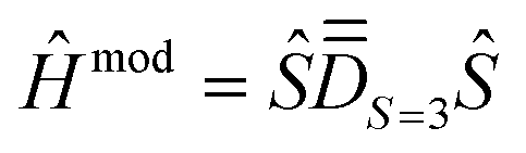 , describing only the ground S = 3 state. A similar strategy was employed for determining the anisotropy axes of [Ni₂(en)₄Cl₂]²⁺.⁶⁵ The procedure consists in:

(i) perform a first reference SOCI calculation with an arbitrary xyz frame, construct the 16 × 16 matrix of Ĥ^eff according to Section 2.2 and focus only on the S = 3 block. This procedure is in essence different from simply following the giant spin approach: in the case of spin mixing, it ensures that we properly extract the actual PAF of the S = 3 block.

(ii) derive the analytical matrix representation of in the |S = 3,M_S〉 space and extract by best equating Ĥ^eff from point (i) to Ĥ^mod. Since this matrix is uncommon in the transition metal literature (an S = 3 state is impossible to reach within a dⁿ manifold), we provide it in Table 1.

Table 1 Matrix elements of expressed in an arbitrary axis frame in the basis of the |S = 3,M_S〉 functions

Ĥ ^mod	|3,3〉	|3,2〉	|3,1〉	|3,0〉	|3,−1〉	|3,−2〉	|3,−3〉
〈3,3|				0	0	0	0
〈3,2|		4Dxx + 4Dyy + 4Dzz			0	0	0
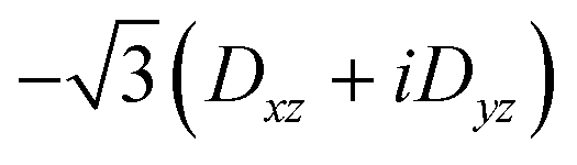
〈3,1|					3Dxx − 3Dyy − 6iDxy	0	0
〈3,0|	0			6Dxx + 6Dyy			0
〈3,−1|	0	0	3Dxx − 3Dyy + 6iDxy
〈3,−2|	0	0	0			4Dxx + 4Dyy + 4Dzz
〈3,−3|	0	0	0	0

---

(iii) rotate the molecular coordinates from the arbitrary xyz frame to the molecular PAF: xyz^MPAF_i = V⁻¹·xyz^arb_i, where xyz^arb_i are the coordinates of all the i atoms in the arbitrary frame and V is the eigenvector matrix of (convention may apply for the respective labeling of the x, y and z axes).

With the molecular geometry rotated in the molecular PAF, the SOCI calculations of Step 1 are repeated and the 16 × 16 representative matrix of Ĥ^eff is re-built. This is the Ĥ^eff that will be essentially used for the validation and resolution of Ĥ^MS. However, note that the exact same conclusions can be reached by extracting it all in an arbitrary axis frame (in a more tedious way!).

Step 2. SOCI calculations are conducted with two model, monomeric, structures defined by the substitution of a magnetic center with a diamagnetic one. In the present cases, models 1a, 1b and 2a, 2b (Fig. 1) are obtained by replacing one Co with one Zn in the dimeric structures 1 and 2 respectively. The goal here is to extract independently the local anisotropy tensors, , for the magnetic centers, determine their respective PAFs, and calculate the corresponding axial and rhombic parameters D_a, E_a, D_b, E_b. For each magnetic center, the eigenvectors of , leading to , provide with the V rotation matrix that can be used to express them back in the molecular PAF, through:

Step 3. The 16 × 16 model analytical matrix of Ĥ^MS in the uncoupled-spin basis is derived with the leading terms of it, i.e., the Heisenberg and the local anisotropy terms, by applying simple spin-operator algebra. This matrix is subsequently transformed in the coupled-spin basis using eqn (3).

Afterwards, the quality of the model matrix can be evaluated by expressing it numerically and comparing it to Ĥ^eff. The less deviation, the better the model. To shortcut the extraction, one may directly use the spin-free J value and the local anisotropy tensors calculated independently at Step 2 (of course, expressed in the molecular PAF for consistency). In principle, this approach should already provide a good representation of Ĥ^eff since (i) the effect of the SOC on J is usually small^30,65 and (ii) the symmetric anisotropy exchange tensor may be of lesser importance than the local ones. Finally, we may also refine the J value and the components of the local anisotropy tensors as well as introduce the symmetric exchange tensor in the model to further improve it. Refinement is carried out through a least-squares fitting of the model parameters, aiming to minimize the root mean square deviation (RMSD) between Ĥ^MS and Ĥ^eff.

Here, we have deliberately chosen to make use of momoner calculations to (i) validate and provide additional support for this route, which is one of the most commonly employed in current literature when modeling magnetic properties, for instance followed by the POLY_ANISO program,^77,78 and (ii) avoid the extraction of too many parameters simultaneously in unsymmetrical cases, such as that of complex 2, thus preventing the occurrence of unnoticed human mistakes by allowing a cross-validation of the extraction procedure based on the much simpler extracted parameters of the monomer calculations. Note that we would be now confident in performing a complete extraction based on a dimer calculation on a new system, or alternatively in performing only monomer calculations if the dimer calculations would prove to be too demanding.

2.4 Computational details

Electronic structure calculations were performed with the ORCA package, v5.0.3.^79,80 Scalar relativistic effects were introduced by using the Douglas–Kroll–Hess (DKH) Hamiltonian.^81–84 The Co, N, O, and Cl electrons were treated with the all-electron, triple-zeta DKH-def2-TZVP basis sets whereas the C, F, and H electrons were treated with the smaller, double-zeta DKH-def2-SVP ones. These bases were derived from the original def2 variants by recontraction within the DKH framework.⁸⁵ To speed off the calculation of electron repulsion integrals, the RIJCOSX “chain-of-spheres” density-fitting⁸⁶ was applied together with large, automatically-generated auxiliary basis sets.⁸⁷ The geometries of 1 and 2 were extracted from published crystal information data.^66,68 Concerning 2, the H coordinates were optimized within the DFT framework, using the Perdew–Burke–Ernzerhof generalized gradient approximation,⁸⁸ and otherwise the same details as above hold. The xyz coordinates in the initial, arbitrary, coordinate frames are provided in the ESI.†

The zero-order wavefunctions were converged within the state-averaged (SA) CASSCF framework, with the active space spanned by the Co(II) d⁷ shell(s). I.e., CASSCF(14, 10) and CASSCF(7, 5) calculations were performed for the dimeric species 1 and 2 and for the monomeric species 1a, 1b, 2a and 2b, respectively. The production-level SA schemes included 49 states per S = 3, 2, 1 and 0 block for 1, seven S = [/] states for 1a and 1b, 9 states per S = 3, 2, 1 and 0 block for 2, three S = [/] states for 2a and 2b. Regarding complex 2 and its monomers, additional SA schemes were explored for validation purposes, which will be discussed in the Results sections. The 49-root per spin-block SA scheme employed for 1 was validated in ref. 67, 49 being the total number of roots generated from the product of the two local (crystal-field split) ⁴F Co(II) terms. Concerning complex 2, the 9-root per spin-block SA scheme has been validated in this work, 9 corresponding to the number of roots generated from the product of two local ⁴T₁ Co(II) terms.

State energies including dynamic correlation effects were calculated with the strongly-contracted, n-electron valence state perturbation theory at second order (NEVPT2).^89,90 For 2 in particular, the relative correlated energies for the lowest S = 3, 2, 1 and 0 states were additionally recorrected by difference dedicated CI (DDCI2) and iterative DDCI2 calculations,^91,92 with an orbital-energy cutoff between −10 and 1000 Hartree and the T_sel and T_pre thresholds set to 1 × 10⁻¹⁰ and 1 × 10⁻⁶, respectively. In this way, a better J value was obtained, or in other words, a better separation of the spin blocks. In the iterative DDCI2 calculation, a limit of ten iterations was employed.

Finally, the production SOCI calculations were performed for all the dimeric and monomeric species. In these calculations, the spin–orbit operator matrix was constructed in the basis of the spin components of the CASSCF states. The SOCI matrix is constituted of off-diagonal elements, triggered by the spin–orbit coupling, and also of diagonal ones, the electronic spin-free energies. The diagonal was dressed with dynamically-correlated energies and the resulting matrix was diagonalized to generate the spin–orbit coupled wavefunctions and energies. Hereafter, SOCI calculations based on NEVPT2 and DDCI2 correlated energies will be referred to as SO-NEVPT2 and SO-DDCI2 respectively. We point out additionally that, in the SO-DDCI2 calculations, only the relative energies of the lowest S = 3, 2, 1, 0 CASSCF states were adjusted by the DDCI2 energy spacings, whereas the NEVPT2 relative energies were retained for the remaining 192 CASSCF states. The intention here was to characterize as best as possible the spin–orbit states that may be populated in the temperature range employed in experimental magnetic susceptibility studies. Since other excited states appear at much higher energies, above 2800 cm⁻¹, they do not contribute much to the observed properties.

Finally, powder-averaged ab initio χT curves were generated for complexes 1 and 2 directly from the outcomes of the SOCI calculations. Note that, in ORCA, χ is calculated by finite differentiation of the partition function by using the (field-corrected) spin–orbit states.⁴⁶ Furthermore, by using the same approach, we have modeled the χT curves based on the pre-validated Ĥ^MS + Ĥ^Zee models, through the usual approximation,

as well as by computing the full χ tensor,where M is the magnetization, B = 0.2 T is the applied magnetic field, α and β are two field directions, is the partition function, and N_A and k_B are the Avogadro and Boltzmann constants, respectively. For the present dicobalt(II) cases, eqn (6) and (7) led to practically identical χT = f(T) model curves.

3 Results and discussion

3.1 [Co₂Cl₆]²⁻, a centrosymmetric complex

3.1.1 Introduction and spin-free spectrum. Magnetic properties in this edge-sharing, bitetrahedral ion were measured by Su et al.⁶⁶ Each Co(II) center adopts an orbitally non-degenerate ground state (GS), ⁴A₂, correlating with the ⁴F ground term of the isolated ion. The χT profile was fitted by an anisotropic model with a relatively large antiferromagnetic Heisenberg exchange coupling, J = 23.2 cm⁻¹ (JŜ_aŜ_b formalism), a large local anisotropy D = 29 cm⁻¹ parameter, and an isotropic g-factor of 2.25. With first-principles calculations, de Graaf and Sousa noted that the anisotropy parameter is well approximated by that of a [CoCl₄]²⁻ structural model.⁶⁷ However, the calculated J value, 34.3 cm⁻¹ with second-order CAS perturbation theory (CASPT2),⁹³ overreached the fitted J. Furthermore, SOCI delivered a low-energy spin–orbit spectrum plagued by a large admixture of septet (S = 3), quintet (S = 2), triplet (S = 1), and singlet (S = 0) spin components. The authors concluded the impossibility of calculating J and D with Ĥ^MS of eqn (1) and reiterated the difficulties of describing magnetic properties in the weak-exchange regime.²¹

Our first-principles calculations support the previous theoretical data. Namely, complex 1 adopts a spin-singlet GS with a Landé ordering for the triplet, quintet, and septet spin-states with antiferromagnetic J of 7.5 (CASSCF)/11.2 cm⁻¹ (NEVPT2). The J value matches that of ref. 67 within 1 cm⁻¹ at the CASSCF level, but it is three times smaller when the dynamic correlation is included. Although the discrepancy may originate from the choice of the PT2 flavor, here NEVPT2 vs. CASPT2 in ref. 67, both these methods deliver similar accuracy when evaluated against the fitted J value of 23.2 cm⁻¹; i.e. if CASPT2 overestimates it by 11.1 cm⁻¹, NEVPT2 underestimates it by 12 cm⁻¹. In this context, DDCI2 calculations led to J = 21.3 cm⁻¹, within ∼2 cm⁻¹ of the fitted value. Iterative DDCI2 calculations did not converge well on a particular value and delivered J within the ∼18–21.5 cm⁻¹ range in 10 iterations, with the mean J = 20.9 cm⁻¹ still in excellent agreement with the fitted J.

3.1.2 Spin–orbit spectrum and determination of the molecular PAF. SOCI calculations were initially performed with complex 1 oriented in the arbitrarily-chosen coordinate frame shown in Fig. 2, i.e. with z and y collinear with the Co₂ and μ-Cl₂ internuclear axis, respectively, and x perpendicular to the Co-(μCl₂)-Co plane. The SOC splits and intercalates the |S,M_S〉 components of the spin-free states, resulting in 16 low-lying levels stretching up to 123 cm⁻¹ (see Table S2, ESI†) and a continuum of excited levels above ∼2700 cm⁻¹. The low-energy spectrum originates almost entirely from SOC admixture of the 16 M_S components of the ground S = 3, 2, 1, and 0 spin-free states. The SO-NEVPT2 wavefunctions listed in Table S3 (ESI†) support this statement and demonstrate that each of these states contains more than 90% summed contributions from such |S,M_S〉 components. This indicates that the majority of the physics is captured by the low-energy ab initio spectrum, which therefore is adequate for the construction of Ĥ^eff and validation of Ĥ^MS.

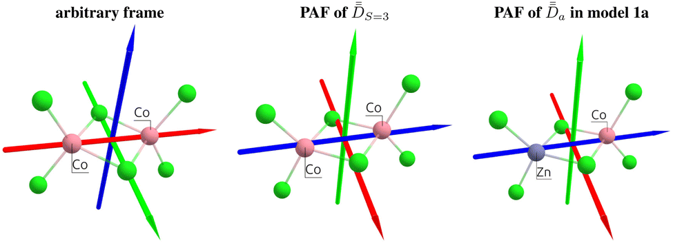Fig. 2 Arbitrarily-chosen coordinate frame and calculated PAFs for complex 1 (from ) and for the model structure 1a (from ). Axes color code: z = red, x = blue, y = green.

Following the strategy presented in Section 2, the first step toward the resolution of Ĥ^MS involves the identification of the molecular PAF. Here, the SOCI wavefunctions of Table S3 (ESI†) already show little spin-mixing due to misalignment of the z-axis with the principal magnetic anisotropy axis of the complex, meaning that the arbitrarily-chosen input frame is not very different from the molecular PAF. The numerical matrix elements of the |S = 3,M_S〉 block within Ĥ^eff are shown in Table 2. Comparison with the analytical matrix of Table 1 concludes with the perfect one-to-one correspondence of the respective matrix elements showing the validity of the model Hamiltonian. Moreover, it is clear that the matrix elements in Ĥ^eff that should vanish in the molecular PAF are very close to zero, e.g. 〈3,2|Ĥ^mod|3,3〉, 〈3,0|Ĥ^mod|3,1〉, etc., meaning that the arbitrary axis frame is indeed not far from the molecular PAF. Indeed, extraction and diagonalization of led to the molecular PAF shown in Fig. 2, which essentially differs from the arbitrary frame by axis relabeling, i.e. z → x, x → y and y → z. SOCI performed with complex 1 oriented in the molecular PAF led to the wavefunctions printed in Table S4 (ESI†); these are slightly cleaner than the previous ones and show large spin-mixings between S = 0 and S = 2 spin-components, and between the S = 1 and S = 3 ones.

Table 2 Matrix elements, in cm⁻¹, of the S = 3 block within the 16 × 16 matrix of Ĥ^eff, constructed from SO-NEVPT2 calculations on complex 1 oriented in the arbitrary coordinate frame

Ĥ ^mod	|3,3〉	|3,2〉	|3,1〉	|3,0〉	|3,−1〉	|3,−2〉	|3,−3〉
〈3,3|	79.0	1.0 + 2.0i	−15.0 − 6.0i	0	0	0	0
〈3,2|	1.0 − 2.0i	87.0	1.0 + 1.0i	−21.0 − 9.0i	0	0	0
〈3,1|	−15.0 + 6.0i	1.0 − 1.0i	92.0	1.0i	−23.0 − 10.0i	0	0
〈3,0|	0	−21.0 + 9.0i	−1.0i	93.0	−1.0i	−21.0 − 9.0i	0
〈3,−1|	0	0	−23.0 + 10.0i	1.0i	92.0	−1.0 − 1.0i	−15.0 − 6.0i
〈3,−2|	0	0	0	−21.0 + 9.0i	−1.0 + 1.0i	87.0	−1.0 − 2.0i
〈3,−3|	0	0	0	0	−15.0 + 6.0i	−1.0 + 2.0i	79.0

---

3.1.3 Extraction and validation of the multispin Hamiltonian. In order to assemble the model matrix of Ĥ^MS (eqn (1)), we must determine at first the local anisotropy tensors, , associated with the two Co centers, and thereof the axial (D_a and D_b) and rhombic (E_a and E_b) local ZFS parameters (which are here respectively equal by symmetry). To this end, SO-NEVPT2 calculations were performed on the monomeric model structures 1a and 1b shown in Fig. 1, both oriented in the molecular PAF determined above. Because of symmetry, one may here skip the computation of 1b. However, doing it has two advantages, (i) it allows one to validate spreadsheets and (ii) it is generally applicable also in cases with no symmetry. Resolution of the anisotropic Hamiltonians, , was achieved following the effective Hamiltonian workflow for mononuclear complexes.⁴⁵ are found identical here, as expected due to the centrosymmetry. Moreover, they are diagonal in the molecular PAF:which shows that share the same PAF. The ZFS parameters derived from matrix (8) are D_a = D_b = 17.4 cm⁻¹ and E_a = E_b = 3.7 cm⁻¹.

The 16 × 16 analytical matrix of Ĥ^MS was initially derived in the uncoupled-spin basis, |M_Sa,M_Sb〉. Subsequently, the matrix was translated into the coupled-spin basis, |S,M_S〉, and it is listed in Tables S5–S7 (ESI†). In the molecular PAF, the Ĥ^MS matrix simplifies greatly to that shown in Table 4, where all elements depend only on the axial and rhombic parameters of the local anisotropies, D_a and E_a (due to centrosymmetry, D_b and E_b can be replaced by D_a and E_a respectively), and of the symmetric exchange anisotropy, D_ab and E_ab. The 16 × 16 Ĥ^eff matrix derived from the SO-NEVPT2 calculation in the molecular PAF is given in Tables S8 and S9 (ESI†) for the coupled- and uncoupled-spin basis respectively.

In a first approximation, one may assume vanishing symmetric anisotropy, i.e. neglect the contribution of D_ab and E_ab to Table 4, and use the calculated J = 11.2, D_a = 17.4 and E_a = 3.7 cm⁻¹ to evaluate Ĥ^MS. The Ĥ^MS numerical matrix expressed in the coupled- and uncoupled-spin bases is shown in Tables S10 and S11 (ESI†), respectively. Concerning the coupled-spin basis, the correspondence between Ĥ^MS and Ĥ^eff matrices is outstanding at first glance. A closer look reveals, however, that the 〈0,0|Ĥ^eff|2,M_S〉 and 〈1,M_S|Ĥ^eff|3,M_S〉 elements, as well as their complex-conjugates, have opposite sign compared to counterparts in Ĥ^MS. The sign discrepancy reported and clarified in the erratum to ref. 4, occurs since the |S,M_S〉 spin functions enter with arbitrary phases in the ab initio spin–orbit eigenvectors, and may show up with random ±1 prefactors between different ab initio runs or runs on different computers. The sign arbitrariness becomes problematic when Ĥ^eff is translated in the uncoupled-spin basis using tabulated CG coefficients that follow a specific sign convention. The ones used in this work, shown in Table S1 (ESI†), follow the Condon and Shortley convention.^94,95 Indeed, comparison between the Ĥ^MS and Ĥ^eff numerical matrices in the uncoupled-spin basis, S11 vs. S9 (ESI†), is rather poor, generating misleading conclusions. In order to obey sign conventions, one may express the spin-free wavefunctions in a basis of localized orbitals, pick a phase convention, and derive analytically the expressions of the spin–orbit wavefunctions; finally, revise the CG coefficients according to the chosen phase convention. This path has been adopted in ref. 74. Pursuing such a scheme, although rigorous, is tedious and not appealing in general. Instead, one may follow the path taken in ref. 4 and revise the conflicting signs in Ĥ^eff such that projection onto Ĥ^MS using CG coefficients in the Condon–Shortley convention gives the smallest deviation. In this work, it is realized from the onset that, by construction, the model Ĥ^MS already yields the correct signs that must be adopted in Ĥ^eff itself. The sign-revised, coupled-spin basis Ĥ^eff is shown in Table S12 (ESI†) and the uncoupled-spin basis matrix derived thereof is shown in Table S13 (ESI†). Comparison with Ĥ^MS counterparts (Tables S10 and S11, ESI†) reveals outstanding agreement regardless of basis, with maximum deviation not larger than 1 and 1.8 cm⁻¹ for the off-diagonal and diagonal elements respectively (see Tables S14 and S15, ESI†). Three highly important conclusions are here drawn, (i) the local anisotropy parameters calculated independently using monomeric structures 1a and 1b are transferable to calculations on the dimeric complex 1, (ii) the local anisotropies are the main contributors to Ĥ^MS and actually bring the model to very close agreement with Ĥ^eff, and (iii) the approximate Ĥ^MS, accounting only for the Heisenberg exchange and local anisotropies, is validated through the effective Hamiltonian theory and may be already used in modeling magnetic properties such as the χT curve.

Prior to modeling the χT curve, it may be noted that the comparison between the analytical matrix of Ĥ^MS (Table 4) and the numerical matrix of Ĥ^eff (Table S12, ESI†) provides with enough equations for a full extraction of all the magnetic parameters at once. Thus, a more precise extraction can be performed on 1 in order to obtain J under the effect of SOC and both the local and the symmetric-exchange anisotropies. Such a full extraction has been performed by least-squares fitting of the Ĥ^MS parameters in order to minimize the RMSD with the Ĥ^eff matrix elements. The extracted parameters, listed in Table 3, lead to Ĥ^MS matrices (Tables S16 and S17, ESI† for the uncoupled- and coupled-spin basis respectively) that agree with Ĥ^eff within 1 cm⁻¹ concerning the off-diagonal and diagonal elements (see Tables S18 and S19, ESI†). Furthermore, diagonalization of the model Ĥ^MS matrices leads to highly accurate spin–orbit energies, within 1.2 and 1.8 cm⁻¹ of the ab initio energies (see Table S2, ESI†), further supporting the validity of Ĥ^MS and of our extraction scheme.

Table 3 Magnetic parameters, in cm⁻¹, obtained from the resolution of Ĥ^MS based on Ĥ^eff's derived from different calculations on complex 1 in the molecular PAF. The isotropic g-factor per Co center, obtained with models 1a and 1b, is also printed

Method	J	D a	E a	D ab	E ab	g
a Obtained from a least-squares fitting procedure minimizing the RMSD between Ĥ^MS and Ĥ^eff. b Recalculated parameters after relabeling of the axes such that the convention Eab > 0 and |Dab| > 3Eab is fulfilled: x → z, y → x, z → y with SO-NEVPT2 and x ↔ z with SO-DDCI2. c From ref. 66.
SO-NEVPT2	10.5	17.13	3.68	0.25^a/−0.64^b	−0.34^a/0.045^b	2.38
SO-DDCI2	19.3	17.32	3.70	0.36^a/−0.71^b	−0.35^a/0.004^b	n/a
Fit^c	23.2	29	—	—	—	2.25

---

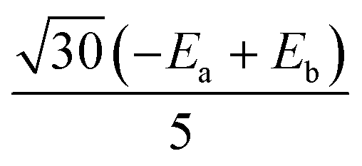
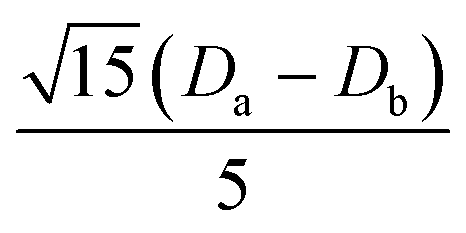
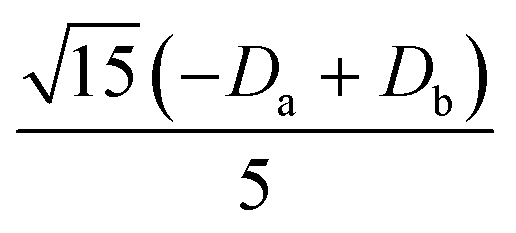
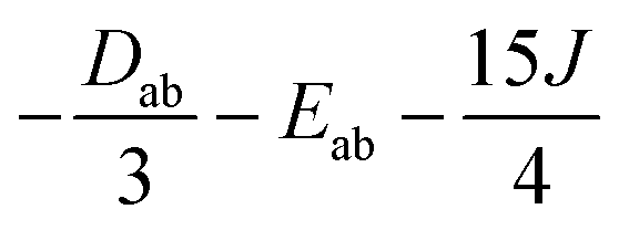
Several aspects may be noted from Table 3: (i) since J only appears on the diagonal of Ĥ^MS in Table 4, switching from NEVPT2 to corrected DDCI2 relative energies affects the J values themselves but leaves mostly unchanged the remaining parameters; the SOC reduces J by 0.7 and 2 cm⁻¹ at the SO-NEVPT2 and SO-DDCI2 levels, respectively, (ii) the re-extracted local anisotropy parameters at the SO-NEVPT2 level, D_a = 17.1 and E_a = 3.7 cm⁻¹ are in complete agreement with the counterparts extracted independently with the 1a and 1b monomeric structures, D_a = 17.4 and E_a = 3.7 cm⁻¹, reaffirming the transferability of these parameters from monomer to dimer calculations, and (iii) the symmetric exchange anisotropy is indeed minor compared to local anisotropies and thus neglecting it from the construction of Ĥ^MS is not a bad approximation. It is worth noting for specialists that re-labeling the axes describing the PAF of is necessary in order to respect the conventions E_ab > 0 and |D_ab| > 3E_ab. In particular, the easy axis of magnetization of the symmetric anisotropy, which is collinear with the Co₂ internuclear axis, falls perpendicular to the molecular easy axis of local anisotropy, which in turn is almost collinear with the μ-Cl₂ internuclear axis.

Table 4 Analytical matrix elements of for binuclear Co(II) complexes in the molecular PAF expressed in the coupled spin-basis, |S,M_S〉

H ^MS	|3,3〉	|3,2〉	|3,1〉	|3,0〉	|3,−1〉	|3,−2〉	|3,−3〉
〈3,3|		0		0	0	0	0
〈3,2|	0		0		0	0	0
〈3,1|		0		0		0	0
〈3,0|	0		0		0		0
〈3,−1|	0	0		0		0
〈3,−2|	0	0	0		0		0
〈3,−3|	0	0	0	0		0
〈2,2|	0	D a − Db	0		0	0	0
〈2,1|		0		0		0	0
〈2,0|	0		0	0	0		0
〈2,−1|	0	0		0		0
〈2,−2|	0	0	0		0	−Da + Db	0
〈1,1|		0		0		0	0
〈1,0|	0		0		0		0
〈1,−1|	0	0		0		0
〈0,0|	0	0	0	0	0	0	0

---

	|2,2〉	|2,1〉	|2,0〉	|2,−1〉	|2,−2〉	|1,1〉	|1,0〉	|1,−1〉	|0,0〉
〈3,3|	0		0	0	0		0	0	0
〈3,2|	D a − Db	0		0	0	0		0	0
〈3,1|	0		0		0		0		0
〈3,0|		0	0	0		0		0	0
〈3,−1|	0		0		0		0		0
〈3,−2|	0	0		0	−Da + Db	0		0	0
〈3,−3|	0	0	0		0	0	0		0
〈2,2|		0		0	0	0		0
〈2,1|	0		0		0		0		0
〈2,0|		0		0		0	0	0
〈2,−1|	0		0		0		0		0
〈2,−2|	0	0		0		0		0
〈1,1|	0		0		0		0		0
〈1,0|		0	0	0		0		0	0
〈1,−1|	0		0		0		0		0
〈0,0|		0		0		0	0	0

---

Finally, the fully extracted Ĥ^MS is used to model the χT curve of complex 1. For this task, one needs to express in matrix form the Zeeman terms of the two magnetic centers, , and add them to Ĥ^MS. Working in the uncoupled-spin basis, the 16 × 16 analytical matrices of the Zeeman terms are derived in Tables S20 and S21 (ESI†). These matrices are evaluated with tensors obtained via the effective Hamiltonian theory from SO-NEVPT2 calculations performed on structures 1a and 1b in the molecular PAF:

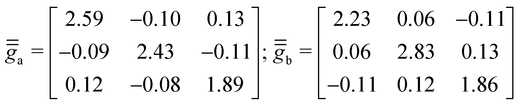
The diagonal form of eqn (9) shows, as expected, that the local PAFs of the tensors also coincide with the molecular PAF. The isotropic g-factor of 2.38 is very close to the fitted value in ref. 66, g = 2.25.

The modeled χT = f(T) curves with magnetic parameters from Table 3, shown in Fig. 3, highlight primarily the role of the magnetic coupling J in achieving agreement with the experiment. Since the J = 10.5 cm⁻¹ extracted from the SO-NEVPT2 calculation is too small, the χT curve increases steadily and diverges from the reference experimental curve. The revised J = 19.3 cm⁻¹ extracted out of the SO-DDCI2 calculation leads to χT in a much closer agreement, especially in the low-temperature range, ∼0–50 K. Furthermore, with a slightly adjusted isotropic g-factor of 2.28, which is even closer to the fitted 2.25 value,⁶⁶ the modeled χT curve with the SO-DDCI2 parameters fits almost perfectly the experimental curve in the whole temperature range. The present article does not aim to delve into higher-level theoretical approaches that could potentially improve the description of g from the onset. Therefore, we conclude that the successful resolution and utilization of the standard multispin model Hamiltonian for calculating magnetic properties in the centrosymmetric complex 1 have been here neatly demonstrated.

Fig. 3 χT = f(T) experimental curve of complex 1, digitized from ref. 66, and modeled with the spin Hamiltonian Ĥ = Ĥ^MS + Ĥ^zee, dressed with parameters listed in Table 3.

3.2 [Co₂(L)₂(acac)₂(H₂O)], an unsymmetrical complex

3.2.1 Introduction and local, Co(II), electronic structures. The μ-O₂(phenoxo)-bridged binuclear complex 2 displays Co(II) centers coordinated by O and N atoms. The local coordination around both metals is near-O_h, with bond angles between 85–96° and Co–O and Co–N mean distances of ∼2.07 and 2.08 Å respectively. Recent work recorded a χT profile consistent with weak ferromagnetic behavior and an interesting maximum below 10 K.⁶⁸ Fitting of the χT curve resulted in J = −3.74 cm⁻¹ (JŜ_aŜ_b convention). The study concluded that overall, the spin alignment is favored by the spin–orbit coupling (SOC) and the local coordination geometry around the metals. It is important to note that the local orbital degeneracy of the 3d t_2g orbitals in O_h leads to non-zero orbital momentum in the Co(II) d⁷ configuration, thus theoretically invalidating the use of the spin Hamiltonian approach. However, we will show here that the local distortions at play in complex 2 are large enough to make the spin Hamiltonian approach relevant. Note that it is possible to generalize our approach to account for orbital momentum, which will be the subject of a dedicated work. Therefore, we begin detailing the local many-electron states at the Co(II) centers as provided by NEVPT2 calculations conducted with the 2a and 2b monomeric structures.

The ground term of the free-ion Co(II), denoted as ⁴F, splits in (weak) O_h ligand fields, resulting in a ground ⁴T₁ state and excited ⁴T₂ and ⁴A₂ states. The threefold degeneracy of the orbital-triplet states is then lifted by distortions of the local O_h coordination. According to Table 5, both Co(II) centers exhibit spin-free energy levels with a ⁴F parentage that are well isolated within specific ranges: approximately 0–1100 cm⁻¹ for ⁴T₁, 8600–10 500 cm⁻¹ for ⁴T₂, and above 18 500 cm⁻¹ for ⁴A₂. The energy variation of these individual levels on the employed SA scheme is minimal. If the overall degeneracy lift of ⁴T₁ is similar for both Co centers (around 1100 cm⁻¹), the splitting of ⁴T₂ is three times larger in 1a (around 1500 cm⁻¹) than in 1b (around 400 cm⁻¹). Taken together with the fact that the spectral widths of the states listed in Table 5 is about 750 cm⁻¹ higher in 2a compared to 2b, these data reflect the slightly more distorted octahedron around the magnetic center of the former structure. Overall, based on energy gaps alone, one may conclude that the three levels of ⁴T₁ parentage are the primary contributors shaping the local spin–orbit electronic structures. Consequently, performing SOC calculations with a SA/SI scheme involving these three quartets should be sufficient to address the local ZFS parameters.

Table 5 Spin-free (SF) and spin–orbit (SO) energies and local magnetic parameters for the Co(II) centers of complex 2, obtained with NEVPT2 calculations and different SA/SI schemes^a

	2a			2b
	10Q + 40D	7Q	3Q	10Q + 40D	7Q	3Q
a Relative energies and ZFS parameters in cm^−1; letters D and Q are used to denote spin-doublet and spin-quartet states; structures 2a and 2b are shown in Fig. 1. b KD in the labeling of the SO states stands for Kramers doublet.
SF
^4T1	0	0	0	0	0	0
	622	600	610	460	446	468
	1079	1044	1059	1175	1143	1154
^4T2	8952	8673	n/a	9189	8895	n/a
	9341	9050	n/a	9352	9059	n/a
	10 555	10 211	n/a	9583	9280	n/a
^4A2	19 969	19 344	n/a	19 190	18 584	n/a
SO^b
KD1	0	0	0	0	0	0
KD2	147	157	178	190	194	205
KD3	721	708	733	664	659	688

---

Local ZFS parameters and isotropic g-factors
	D a	E a	g a	D b	E b	g b
	86.31	11.91	2.30	93.14	25.02	2.31

---

Indeed, we found that the lowest-energy Kramers doublets (KDs) only marginally change when increasing the SA/SI scheme beyond the first three quartet roots. As listed in Table 5, each Co(II) center exhibits one KD below approximately 200 cm⁻¹ and the others above 700 cm⁻¹. Evidently, all these Kramers doublets (KDs) fully arise as admixtures of |S = [/],M_S〉 components of the spin-free states correlating with ⁴T₁. Furthermore, the spin-free quartet GS predominantly contributes to the wavefunctions of KD₁ (∼75%) and KD₂ (∼90%) in both 2a and 2b. The next significant contribution to KD₁, approximately 20%, comes from the first excited spin-quartet root. Anyway, one can confidently extract local ZFS parameters from the usual anisotropic spin Hamiltonians , expressed in the |S = [/],M_S〉 basis of the ground quartet state (the model space thus consisting of the leading contributors to both KD₁ and KD₂).

The extracted axial, D_a and D_b, and rhombic, E_a and E_b, ZFS parameters are listed at the bottom of Table 5. The PAFs of the local rank-2 tensors, , shown in Fig. 4, are very distinct this time, with orientations that may not have been guessed without performing those calculations. In comparison with complex 1, the axial parameters D_a/b ≃ 90 cm⁻¹ are at least fivefold larger. Furthermore, E_b = 25 cm⁻¹ is twice larger than E_a = 12 cm⁻¹, and both are at least three times larger than the local rhombic parameter in complex 1, 3.7 cm⁻¹. On another hand, the Co centers share similar isotropic g-factor, g_a ≃ g_b ≃ 2.30, with that of the Co centers in complex 1, g_a = g_b = 2.35. Here, however, the spans of , 1.86–2.66 and 1.81–2.84 respectively, are much larger than the -tensor span in complex 2, 2.23–2.40, also highlighting the much larger anisotropy in complex 2 in terms of the local 's.

Fig. 4 Arbitrarily-chosen coordinate frame and calculated PAFs for complex 2 (from ) and for the model structures 2a (from ) and 2b (from ). Axes color code: x = blue, y = green, z = red.

3.2.2 Spin-free and spin–orbit spectra and determination of the molecular PAF. Calculations for complex 2 were initially performed in an arbitrary coordinate system (see Fig. 4, the Co₂ and μ-O₂ internuclear axis correspond to the z and y directions, respectively, and the x axis is perpendicular to the Co-[μO₂]-Co plane). Spin-free NEVPT2 calculations were conducted, revealing a Landé type spectrum with an S = 3 GS followed by a first set of S = 2, 1 and 0 excited states, mapped with a ferromagnetic J (−2.85 cm⁻¹). This value is within 1 cm⁻¹ of the J = −3.74 cm⁻¹ obtained from fitting the experimental χT curve.⁶⁸ When considering the SOC, there are 16 lowest-lying energy levels within 389 cm⁻¹ (see Table 7 and Table S22, ESI†). In comparison to complex 1, not only is this energy range three times larger, but the continuum of excited levels begins at a much lower energy, 691 cm⁻¹. Importantly, the total contribution of the lowest-energy S = 3, 2, 1, 0 spin-free states to the wavefunctions of those 16 spin–orbit levels gradually increases, from about 50% in Ψ₁ to 81% in Ψ₁₆. Although these weights are lower than what was observed in 1, it should be noted that the SOCI wave functions are still dominated by the standard model space (the projection on the model space being more than 50%) and that in fine will we show that our approach allows us to reproduce accurately the experimental χT curve.

A quick look at Table S23 (ESI†) reveals that the wavefunctions of the 16 lowest-lying spin–orbit levels are plagued by spin-mixing, which may be less important if the molecular PAF is used. We proceeded, therefore, as before to derive the molecular PAF. The matrix elements of the S = 3 block within the 16 × 16 Ĥ^eff, shown in Table 6, perfectly match the Ĥ^mod analytical matrix elements listed in Table 1. Unlike in the previous case of complex 1, matrix elements such as 〈3,2|Ĥ^eff|3,3〉 or 〈3,1|Ĥ^eff|3,2〉 deviate significantly from zero, whereas they should be zero if the input xyz frame is the molecular PAF. Extraction and diagonalization of led to the molecular PAF depicted in Fig. 4. This frame is not only distinct from the initial input frame but also distinct from the local PAFs (of ). The SO-NEVPT2 calculation was repeated in the molecular PAF, leading to much cleaner wavefunctions for the 16 lowest-lying energy levels (see Table S24, ESI†).

Table 6 Matrix elements, in cm⁻¹, of the S = 3 block within the 16 × 16 matrix of Ĥ^eff, constructed from SO-NEVPT2 calculations on complex 2 in the arbitrary coordinate frame

Ĥ ^mod	|3,3〉	|3,2〉	|3,1〉	|3,0〉	|3,−1〉	|3,−2〉	|3,−3〉
〈3,3|	134.0	18.0 + 44.0i	5.0 + 62.0i	0	0	0	0i
〈3,2|	18.0 − 44.0i	188.0	14.0 + 34.0i	8.0 + 88.0i	0	0	0
〈3,1|	5.0 − 62.0i	14.0 − 34.0i	221.0	5.0 + 13.0i	8.0 + 97.0i	0	0
〈3,0|	0	8.0 − 88.0i	5.0 − 13.0i	232.0	−5.0 − 13.0i	8.0 + 88.0i	0
〈3,−1|	0	0	8.0 − 97.0i	−5.0 + 13.0i	221.0	−14.0 − 34.0i	5.0 + 62.0i
〈3,−2|	0	0	0	8.0 − 88.0i	−14.0 + 34.0i	188.0	−18.0 − 44.0i
〈3,−3|	0	0	0	0	5.0 − 62.0i	−18.0 + 44.0i	134.0

---

Table 7 Low-energy spin–orbit spectrum of complex 2^a

SO state	ΔE		SO state	ΔE
a SO-NEVPT2 calculations, relative energies in cm^−1. Other excited energy levels start at 691 cm^−1. b Total contribution from the spin-components of the lowest-energy S = 3, 2, 1 and 0 spin-free states.
Ψ 1	0	0.52	Ψ 9	206.4	0.66
Ψ 2	1.9	0.51	Ψ 10	206.9	0.67
Ψ 3	3.6	0.50	Ψ 11	209.6	0.65
Ψ 4	7.7	0.50	Ψ 12	212.2	0.66
Ψ 5	177.0	0.62	Ψ 13	379.7	0.80
Ψ 6	177.7	0.64	Ψ 14	380.0	0.80
Ψ 7	180.7	0.64	Ψ 15	388.4	0.69
Ψ 8	182.2	0.61	Ψ 16	389.0	0.81

---

3.2.3 Extraction of the multispin Hamiltonian. Fig. 4 clearly highlights that the local anisotropy tensors, , cannot be diagonal in the molecular PAF. Since our procedure does not require any assumption on the local PAFs, we have re-computed (rotated) them in the molecular PAF prior to assembling Ĥ^MS according to eqn (1):

It should be stressed that no specific relationship appears between the elements of these tensors, in accord with the C₁ symmetry point group of complex 2.

We are now in the position to best equate the 16 × 16 matrix of Ĥ^MS with the representative matrix of Ĥ^eff. We first consider the expressions reported in Tables S5 and S6 (ESI†), meaning that we neglect the symmetric exchange tensor. By using the −2.85 cm⁻¹ spin-free J value and the full tensors (eqn (10)), the estimated numerical matrix of Ĥ^MS is given in Tables S25 and S26 (ESI†) in the uncoupled |M_Sa,M_Sb〉 and coupled |S,M_S〉 spin basis, respectively. These are brought in correspondence with the effective Hamiltonians shown in Tables S27 (coupled-spin basis) and S28 (uncoupled-spin basis) (ESI†). As was the case with complex 1, outstanding agreement is obtained from the comparison regardless of the spin basis. Indeed, the difference between Ĥ^eff and Ĥ^MS is already smaller than 1 and 2.7 cm⁻¹ concerning the off-diagonal and diagonal matrix elements, respectively. It is worth emphasizing once again that the independently calculated local anisotropy tensors, , within the framework of the 2a and 2b monomeric structures, can be safely transferred to the dimeric structure 2.

As with complex 1, we proceeded to extract J under the influence of SOC, as well as the symmetric anisotropy tensor , without revising the local anisotropies. In other words, we constructed Ĥ^MS as follows:

where “mono” refers to the monomer calculations. The contribution of , expressed in an arbitrary axis frame and in the coupled-spin basis, is displayed in Table S7 (ESI†). The contribution of in its own PAF is given in Table S31 (ESI†). A careful inspection of all the relevant tables revealed that in fact the previous deviations between the estimated Ĥ^MS and Ĥ^eff can essentially be explained by Table S31 (ESI†). In other words, the PAF of practically matches the molecular PAF, and thus we only need to fit the J, D_ab, and E_ab parameters to refine Ĥ^MS.

Table 8 summarizes all the key magnetic parameters resulting from the resolution of Ĥ^MS for the case of complex 2 (we recall that the tensors are not diagonal in the molecular PAF). In the coupled-spin basis, the numerical matrix of Ĥ^MS is shown in Table S32 (ESI†). This model is of course in even better agreement with the effective Hamiltonian (Table S27, ESI†). The difference matrix between Ĥ^MS and Ĥ^eff, displayed in Table S33 (ESI†), now shows that all the elements are generally smaller than 1 cm⁻¹. Furthermore, diagonalization of our model Ĥ^MS yields highly accurate spin–orbit energies, with an average deviation of only 1.2 cm⁻¹ and a maximum deviation of 2.6 cm⁻¹. Consequently, we have successfully applied our new procedure to properly extract all the rank-2 tensors of Ĥ^MS and, ultimately, validated the standard multispin Hamiltonian for any binuclear complex since the key step of unsymmetrical dicobalt(II) complexes is now solved.

Table 8 Magnetic parameters, in cm⁻¹, obtained from the complete resolution of Ĥ^MS for complex 2 oriented in the molecular PAF

J	D ab	E ab	D a	E a	D b	E b
a Generated from a least-squares fitting of the model parameters in order to minimize the RMSD between Ĥ^MS and Ĥ^eff. b Recalculated parameters after relabeling of the MPAF axes such that the convention Eab > 0 and |Dab| > 3Eab is fulfilled: y → z, z → x, x → y.
−2.28	−0.07^a/0.22^b	−0.13^a/0.03^b	86.31	11.91	93.14	25.02

---

Finally, we take a step forward and attempt to model the powder-averaged χT profile of complex 2 using the validated Ĥ^MS. For this purpose, we use again the analytical expressions of the Zeeman Hamiltonians, derived in Tables S20 and S21 (ESI†), using the tensors obtained with the 2a and 2b structural models, based on calculations performed in the molecular PAF:

Those matrices are not diagonal in the molecular PAF and in fact, the corresponding local PAFs also do not strictly match one another (as was observed for ). Since the off-diagonal elements are smaller than the diagonal ones in eqn (12), one can still consider that are close to being diagonal in the molecular PAF, even if a detailed analysis may reveal an interchange between the respective hard and intermediate axes of magnetization between .

Fig. 5, top panel, demonstrates the excellent agreement between the reference, experimental χT curve⁶⁸ and the one obtained directly out of the SO-NEVPT2 calculation. Therefore, we can be confident in the quality of our ab initio calculations and now aim at producing good quality model curves, in view of further supporting the validity of both Ĥ^MS and of our procedure to extract the magnetic parameters. The model curve, obtained from Ĥ^MS + Ĥ^Zee dressed with quantities from Table 8 and eqn (12), agrees with the reference data in the low-temperature region. As the temperature increases, it deviates more and more, eventually reaching a plateau around 150 K which is quite lower than the experimental curve. The behavior may be caused by (i) the lack of excited states in our model that may be populated at some point and in particular at 300 K and (ii) an underestimation of the isotropic g value for each Co center. Concerning point (i), the sum of the Boltzmann populations of the first 16 energy levels is 94% at 300 K. We hypothesize that the remaining 6% in terms of population are not mandatory to explain the discrepancy between this first model curve and the ab initio one. Furthermore, it appears that the model curve is too low for a much larger temperature range, in particular from 30 to 300 K. At 30 K, it is clear that only the first 16 energy levels are populated, hence the problem may fully lie on the isotropic g values, as was observed in complex 1 (in this case, the isotropic g value had to be tempered to a lower value). By following this hypothesis, we here need to increase the isotropic g value, which leads to a revised model curve that is more satisfactory for the whole 30–300 K problematic range, without compromising the already good 0–30 K range. The fitted g = 2.55 value is not completely random as it may be justified based on the measured room-temperature χT value of 6.03 cm³ mol⁻¹ K, or rather 3.015 cm³ mol⁻¹ K per Co center, according to:

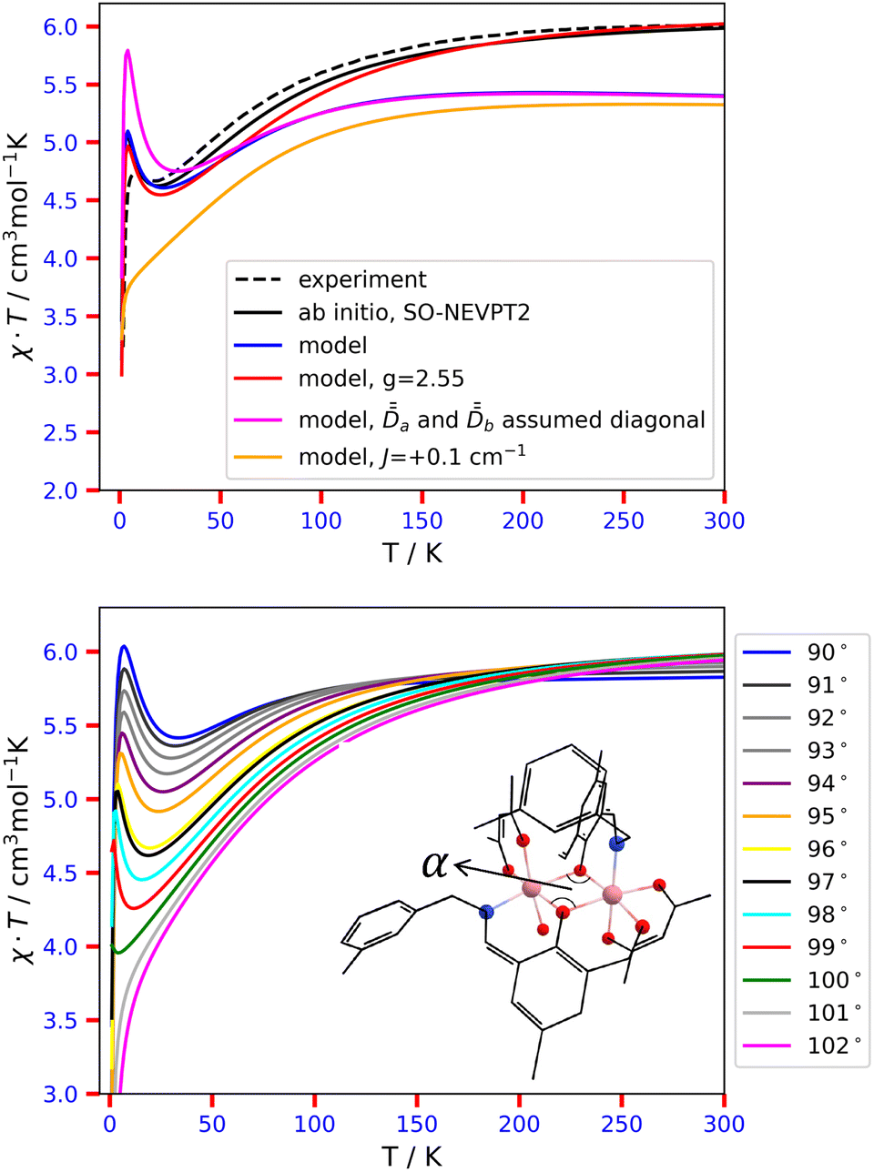Fig. 5 Top: Experimental χT = f(T) curve of complex 2, digitized from ref. 68, and generated from ab initio calculations and multispin Hamiltonian models. Bottom: χT = f(T) curves obtained with SO-NEVPT2 as a function of the angle α° = ∠Co–O–Co. In the crystal structure, α = 97°, and the black curve represents the best approximation of the experimental χT.

This expression leads to g = 2.54 with the Boltzmann constant, k_B = 0.695 cm⁻¹ K⁻¹, μ_B = 0.467, cm⁻¹ T⁻¹, and N_A·μ_B = 0.558 cm³ mol⁻¹ T. Note that since our main point here is to understand the zero-field behavior, we do not aim to delve deeper into explaining the reasons behind this revision of the SO-NEVPT2 g value.

Two additional models are displayed in Fig. 5, top panel, evidencing the shape of χT if one assumes that the local anisotropy tensors are diagonal in the molecular frame and if the axial and rhombic parameters displayed in Table 8 are used, or if J is artificially set to a weakly antiferromagnetic value. The first scenario artificially pushes up the model curve in the low-temperature range, meaning that the maximum is too high. While it is quite intuitive that the mismatch of the actual PAFs of the local anisotropy tensors should lower the model curve, we should stress that if one assumes that the tensors are diagonal in the molecular PAF and if one fits the local ZFS parameter values, as could be done to fit the experimental data, this should lead to too weak ZFS parameters. In other words, it is crucial to account for the mismatch of the local PAFs in the model, otherwise, meaningless parameters would be obtained. This is exactly where experimental extractions of Ĥ^MS parameters should not be performed independently from computational chemistry data.

We now aim to better explain the occurrence of a local maximum of χT at low temperatures. From the previous paragraph, we have learned that the mismatch between the local PAFs works towards lowering this χT maximum. Such maximum does not occur if the antiferromagnetic coupling scenario is retained (see Fig. 5). Thus, one could naively think that J must be maximized to favor the occurrence of such a maximum. In practice, to get a local maximum of χT, we believe that it requires population of a state that is much less magnetic than the ones before and after it. A close inspection of Table S24 (ESI†) reveals that the fourth spin–orbit level is essentially derived from the M_S = 0 components of the spin-quintet and spin-singlet states so that this must be the states that are looked for. For this state to occur in between the components of the S = 3 state, one needs to be in the weak-exchange limit (note that this also strengthens the spin-mixing with the singlet state, which also pushes down this state in the model). Additionally, this state must be well separated in energy from the subsequent states, otherwise, a continuous enhancement of χT would be observed. According to Table 7, a gap of about 170 cm⁻¹ occurs in complex 2, which corroborates our interpretation.

To strengthen the conclusion drawn earlier, the bottom panel of Fig. 5 illustrates the variation of χT, obtained directly from SO-NEVPT2 calculations, as a function of the Co–O–Co angles. At the crystal-structure value of 97°, the calculated curve best approximates the reference data. Angles below 97° promote stronger ferromagnetic coupling (without getting rid of the weak exchange regime). Consequently, as the “less magnetic” state shifts toward higher energies, the spike in χT is both enhanced and slightly shifted to higher temperatures. On the other hand, angles above 100° promote antiferromagnetism. As a result, the χT curves no longer exhibit local maxima. The overall structural change, induced when the Co–O–Co angle is changed from 97 to, for instance, 101°, is characterized by an RMSD of 0.08 Å, it is thus negligible. Therefore, one can regard the unfolding of χT in complex 2 as an intermediate between the ferromagnetic and antiferromagnetic regimes. This is due to the fact that even a tiny displacement in the molecular structure promptly alters χT, transitioning between these two regimes.

3.3 Reinterpretation of the [Ni₂(en)₄Cl₂]²⁺ case, a centrosymmetric dinickel(II) complex in the weak-exchange regime

An accurate determination of magnetic parameters in [Ni(en)₄Cl₂]Cl₂ has been reported more than a decade ago in the context of high-field EPR experiments.⁹⁶ The complex is weakly ferromagnetic, with J = −9.66, D_a = −4.78, and D_ab = −0.64 cm⁻¹. Maurice et al. performed an extraction of these parameters from the anisotropic multispin Hamiltonian through the effective Hamiltonian theory.⁶⁵ The generated parameters, J = −5.415, D_a = −9.437, E_a = 2.042, D_ab = 0.367 and E_ab = −0.052 cm⁻¹, which are in reasonable agreement with the experimental counterparts, allow for the derivation of the Ĥ^MS numerical matrix listed in Table 9. Comparison with the numerical Ĥ^eff matrix, reproduced from ref. 65 in Table 10, shows outstanding agreement down to only ±prefactors for the elements coupling the S = 2 and S = 0 blocks in Ĥ^eff. Performing a basis-change to the uncoupled basis using tabulated CG coefficients following the Condon–Shortley convention, these conflicting signs lead to unexpected matrix elements, such as 〈1,−1|Ĥ^eff|−1,1〉 = 8.6 cm⁻¹, that should be null according to the standard Ĥ^MS.⁶⁵ As discussed in this article, in ab initio calculations, the conflicting signs arise from arbitrary phases and must be adjusted based on the model matrix. This sign adjustment results in a nearly identical model and effective matrices in both the coupled-spin and uncoupled-spin bases, thereby fully validating the standard multispin Hamiltonian for [Ni(en)₄Cl₂]Cl₂. Consequently, in this context, the introduction of a rank-4, biquadratic exchange tensor, in Ĥ^MS is no longer crucial, unless high accuracy is sought after. Therefore, it is important to stress that the weak-exchange limit was correctly solved in the previous experimental and theoretical works.^65,96 However, the experimental extraction was based on the assumption that rhombicity is negligible, which is not supported by the calculations. Therefore, the experimental J = −9.66, D_a = −4.78, and D_ab = −0.64 cm⁻¹ values may be the subject of small uncertainties due to the neglect of rhombicity, though the important features (weak-exchange limit, local easy-axis anisotropies, |D_ab| < |D_a|) are now no doubt.

Table 9 Numerical matrix elements, in cm⁻¹, of Ĥ^MS for the [Ni₂(en)₄Cl₂]²⁺ complex in the coupled-spin basis^a

Ĥ ^MS	|2,2〉	|2,1〉	|2,0〉	|2,−1〉	|2,−2〉	|1,1〉	|1,0〉	|1,−1〉	|0,0〉
a Obtained by evaluating the analytical expressions reported by ref. 65.
〈2,2|	1.67	0.00	1.62	0.00	0.00	0.00	0.00	0.00	2.39
〈2,1|	0.00	10.74	0.00	1.99	0.00	0.00	0.00	0.00	0.00
〈2,0|	1.62	0.00	13.76	0.00	1.62	0.00	0.00	0.00	−9.07
〈2,−1|	0.00	1.99	0.00	10.74	0.00	0.00	0.00	0.00	0.00
〈2,−2|	0.00	0.00	1.62	0.00	1.67	0.00	0.00	0.00	2.39
〈1,1|	0.00	0.00	0.00	0.00	0.00	21.81	0.00	−2.09	0.00
〈1,0|	0.00	0.00	0.00	0.00	0.00	0.00	12.01	0.00	0.00
〈1,−1|	0.00	0.00	0.00	0.00	0.00	−2.09	0.00	21.81	0.00
〈0,0|	2.39	0.00	−9.07	0.00	2.39	0.00	0.00	0.00	23.96

---

Table 10 Numerical matrix elements of Ĥ^eff expressed in the coupled-spin basis for the [Ni₂(en)₄Cl₂]²⁺ complex in the molecular PAF^a

Ĥ ^MS	|2,2〉	|2,1〉	|2,0〉	|2,−1〉	|2,−2〉	|1,1〉	|1,0〉	|1,−1〉	|0,0〉
a Reproduced from ref. 65.
〈2,2|	1.67	0.00	1.62	0.00	0.00	0.00	0.00	0.00	−2.37 + 0.02i
〈2,1|	0.00	10.74	0.00	1.99	0.00	0.00	0.00	0.00	−0.02 − 0.09i
〈2,0|	1.62	0.00	13.79	0.00	1.62	0.00	0.00	0.00	9.06
〈2,−1|	0.00	1.99	0.00	10.74	0.00	0.00	0.00	0.00	0.02 − 0.09i
〈2,−2|	0.00	0.00	1.62	0.00	1.67	0.00	0.00	0.00	−2.37 − 0.02i
〈1,1|	0.00	0.00	0.00	0.00	0.00	21.81	0.02 + 0.07i	−2.10 + 0.03i	0.00
〈1,0|	0.00	0.00	0.00	0.00	0.00	0.02 − 0.07i	12.02	−0.02 − 0.07i	0.00
〈1,−1|	0.00	0.00	0.00	0.00	0.00	−2.10 − 0.03i	−0.02 + 0.07i	21.81	0.00
〈0,0|	−2.37 − 0.02i	−0.02 + 0.09i	9.06	0.02 + 0.09i	−2.37 + 0.02i	0.00	0.00	0.00	24.12

---

4 Conclusion

By studying dicobalt(II) complexes, we have confirmed the validity of the standard Ĥ^MS independent from the weak- or strong-exchange regime. Using ab initio calculations, we have demonstrated that it is possible to extract the full tensors that make up the model, without making any assumptions about their principal axis frames (PAFs). Furthermore, the analysis, based on model χT curves, has revealed that assuming the local anisotropy tensors are diagonal in the molecular PAF should lead to erroneous local anisotropy parameters in the fitting process. Therefore, concerning unsymmetrical or low-symmetry binuclear complexes, a rigorous interpretation of low-temperature magnetic data should retain key inputs from quantum mechanical calculations similar to those used in this work, i.e. multiconfigurational and relativistic wave functions methods. We hope that the present article will trigger new joint theory/experiment studies based on this renewed perspective of explicitly mapping ab initio data onto Ĥ^MS.

Author contributions

RM conceived the study. DCS, RM and BLG secured funding. DCS performed all the theoretical calculations and implemented all codes utilized in generating the data reported in this manuscript. All authors were equally involved in the data analysis. DCS wrote the first draft of the manuscript. RM and BLG shaped the final form of the manuscript.

Conflicts of interest

There are no conflicts to declare.

Acknowledgements

DCS acknowledges support from the European Unions Horizon 2020 Research and Innovation Program under the Marie Sklodowska-Curie Grant Agreement No. 899546, through the BIENVENÜE COFUND program. DCS also acknowledges the infrastructure support provided through the RECENT AIR grant agreement MySMIS no. 127324.

Notes and references

1. C. A. Goodwin, F. Ortu, D. Reta, N. F. Chilton and D. P. Mills, Molecular magnetic hysteresis at 60 kelvin in dysprosocenium, Nature, 2017, 548, 439–442.
2. F.-S. Guo, B. M. Day, Y.-C. Chen, M.-L. Tong, A. Mansikkamäki and R. A. Layfield, A Dysprosium Metallocene Single-Molecule Magnet Functioning at the Axial Limit, Angew. Chem., Int. Ed., 2017, 56, 11445–11449.
3. F.-S. Guo, B. M. Day, Y.-C. Chen, M.-L. Tong, A. Mansikkamäki and R. A. Layfield, Magnetic hysteresis up to 80 kelvin in a dysprosium metallocene single-molecule magnet, Science, 2018, 362, 1400–1403.
4. C. A. Gould, K. R. McClain, D. Reta, J. G. C. Kragskow, D. A. Marchiori, E. Lachman, E.-S. Choi, J. G. Analytis, R. D. Britt, N. F. Chilton, B. G. Harvey and J. R. Long, Ultrahard magnetism from mixed-valence dilanthanide complexes with metal-metal bonding, Science, 2022, 375, 198–202.
5. L. Bogani and W. Wernsdorfer, Molecular spintronics using single-molecule magnets, Nat. Mater., 2008, 7, 179–186.
6. E. Coronado, Molecular magnetism: from chemical design to spin control in molecules, materials and devices, Nat. Rev. Mater., 2020, 5, 87–104.
7. A. Moneo-Corcuera, D. Nieto-Castro, J. Cirera, V. Gómez, J. Sanjosé-Orduna, C. Casadevall, G. Molnár, A. Bousseksou, T. Parella, J. M. Martínez-Agudo, J. Lloret-Fillol, M. H. Pérez-Temprano, E. Ruiz and J. R. Galán-Mascarós, Molecular memory near room temperature in an iron polyanionic complex, Chem, 2023, 9, 377–393.
8. D. Gatteschi and R. Sessoli, Quantum Tunneling of Magnetization and Related Phenomena in Molecular Materials, Angew. Chem., Int. Ed., 2003, 42, 268–297.
9. W. Wernsdorfer, N. E. Chakov and G. Christou, Quantum Phase Interference and Spin-Parity in Mn₁₂ Single-Molecule Magnets, Phys. Rev. Lett., 2005, 95, 037203.
10. C. Schlegel, J. van Slageren, M. Manoli, E. K. Brechin and M. Dressel, Direct Observation of Quantum Coherence in Single-Molecule Magnets, Phys. Rev. Lett., 2008, 101, 147203.
11. N. Ishikawa, M. Sugita and W. Wernsdorfer, Quantum Tunneling of Magnetization in Lanthanide Single-Molecule Magnets: Bis(phtalocyianato)terbium and Bis(phtalocyianato)dysprosium Anions, Angew. Chem., Int. Ed., 2005, 44, 2931–2935.
12. D. N. Woodruff, R. E. P. Winpenny and R. A. Layfield, Lanthanide Single-Molecule Magnets, Chem. Rev., 2013, 113, 5110–5148.
13. N. Ishikawa, M. Sugita, T. Ishikawa, S.-Y. Koshihara and Y. Kaizu, Lanthanide Double-Decker Complexes Functioning as Magnets at the Single-Molecular Level, J. Am. Chem. Soc., 2003, 125, 8694–8695.
14. Z. Zhu, M. Guo, X.-L. Li and J. Tang, Molecular magnetism of lanthanide: Advances and perspectives, Coord. Chem. Rev., 2019, 378, 350–364.
15. S. T. Liddle and J. van Slageren, Improving f-element single molecule magnets, Chem. Soc. Rev., 2015, 44, 6655–6669.
16. N. F. Chilton, Design Criteria for High-Temperature Single-Molecule Magnets, Inorg. Chem., 2015, 54, 2097–2099.
17. X.-Y. Wang, C. Avendaño and K. R. Dunbar, Molecular magnetic materials based on 4d and 5d transition metals, Chem. Soc. Rev., 2011, 40, 3213–3238.
18. A. Swain, A. Sen and G. Rajaraman, Are lanthanide-transition metal direct bonds a route to achieving new generation 3d-4f SMMs?, Dalton Trans., 2021, 50, 16099–16109.
19. V. Chandrasekhar, Lanthanide and transition metal complexes as molecular magnets, Dalton Trans., 2022, 51, 4199–4201.
20. M. Magott, M. Brzozowska, S. Baran, V. Vieru and D. Pinkowicz, An intermetallic molecular nanomagnet with the lanthanide coordinated only by transition metals, Nat. Commun., 2022, 13, 2014.
21. R. Boča, Zero-field splitting in metal complexes, Coord. Chem. Rev., 2004, 248, 757–815.
22. R. Maurice, R. Broer, N. Guihéry and C. de Graaf, in Zero-Field Splitting in Transition Metal Complexes: Ab Initio Calculations, Effective Hamiltonians, Model Hamiltonians, and Crystal-Field Models, ed. W. Liu, Springer Berlin Heidelberg, Berlin, Heidelberg, 2016, pp. 1–31.
23. I. d P. R. Moreira, N. Suaud, N. Guihéry, J. P. Malrieu, R. Caballol, J. M. Bofill and F. Illas, Derivation of spin Hamiltonians from the exact Hamiltonian: Application to systems with two unpaired electrons per magnetic site, Phys. Rev. B: Condens. Matter Mater. Phys., 2002, 66, 134430.
24. N. F. Chilton, R. P. Anderson, L. D. Turner, A. Soncini and K. S. Murray, PHI: A powerful new program for the analysis of anisotropic monomeric and exchange-coupled polynuclear d- and f-block complexes, J. Comput. Chem., 2013, 34, 1164–1175.
25. J. J. Borrás-Almenar, J. M. Clemente-Juan, E. Coronado and B. S. Tsukerblat, MAGPACK A package to calculate the energy levels, bulk magnetic properties, and inelastic neutron scattering spectra of high nuclearity spin clusters, J. Comput. Chem., 2001, 22, 985–991.
26. W. Z. Heisenberg, Mehrkörperproblem und Resonanz in der Quantenmechanik, Z. Phys., 1926, 38, 411.
27. P. A. M. Dirac, Quantum mechanics of many-electron systems, Proc. R. Soc. London, 1929, 123, 714.
28. J. H. Van Vleck, The theory of electric and magnetic susceptibility, Oxford University Press, United Kingdom, 1932.
29. R. Maurice, C. de Graaf and N. Guihéry, Magnetic anisotropy in binuclear complexes in the weak-exchange limit: From the multispin to the giant-spin Hamiltonian, Phys. Rev. B: Condens. Matter Mater. Phys., 2010, 81, 214427.
30. R. Maurice, A. M. Pradipto, N. Guihéry, R. Broer and C. de Graaf, Antisymmetric Magnetic Interactions in Oxo-Bridged Copper(II) Bimetallic Systems, J. Chem. Theory Comput., 2010, 6, 3092–3101.
31. R. Maurice, K. Sivalingam, D. Ganyushin, N. Guihéry, C. de Graaf and F. Neese, Theoretical Determination of the Zero-Field Splitting in Copper Acetate Monohydrate, Inorg. Chem., 2011, 50, 6229–6236.
32. F. Gendron, J. Autschbach, J.-P. Malrieu and H. Bolvin, Magnetic Coupling in the Ce(III) Dimer Ce₂ (COT)₃, Inorg. Chem., 2019, 58, 581–593.
33. R. Maurice, T. Mallah and N. Guihéry, in Magnetism in Binuclear Compounds: Theoretical Insights, ed. P. Kalck, Springer International Publishing, Cham, 2023, pp. 207–233.
34. L. F. Chibotaru and L. Ungur, Ab initio calculation of anisotropic magnetic properties of complexes. I. Unique definition of pseudospin Hamiltonians and their derivation, J. Chem. Phys., 2012, 137, 064112.
35. A. Wilson, J. Lawrence, E.-C. Yang, M. Nakano, D. N. Hendrickson and S. Hill, Magnetization tunneling in high-symmetry single-molecule magnets: Limitations of the giant spin approximation, Phys. Rev. B: Condens. Matter Mater. Phys., 2006, 74, 140403.
36. R. Boča, Theoretical Foundations of Molecular Magnetism, Elsevier, Amsterdam, 1999, pp. 642–680.
37. B. O. Roos, P. R. Taylor and P. E. M. Siegbahn, A Complete Active Space SCF method (CASSCF) using a density matrix formulated super-CI approach, Chem. Phys., 1980, 48, 157–173.
38. J. P. Malrieu, R. Caballol, C. J. Calzado, C. de Graaf and N. Guihéry, Magnetic Interactions in Molecules and Highly Correlated Materials: Physical Content, Analytical Derivation, and Rigorous Extraction of Magnetic Hamiltonians, Chem. Rev., 2014, 114, 429–492.
39. P.-A. Malmqvist, B. O. Roos and B. Schimmelpfennig, The restricted active space (RAS) state interaction approach with spin–orbit coupling, Chem. Phys. Lett., 2002, 357, 230–240.
40. C. J. Calzado, J. Cabrero, J. P. Malrieu and R. Caballol, Analysis of the magnetic coupling in binuclear complexes. I. Physics of the coupling, J. Chem. Phys., 2002, 116, 2728–2747.
41. C. J. Calzado, J. Cabrero, J. P. Malrieu and R. Caballol, Analysis of the magnetic coupling in binuclear complexes. II. Derivation of valence effective Hamiltonians from ab initio CI and DFT calculations, J. Chem. Phys., 2002, 116, 3985–4000.
42. R. Broer, L. Hozoi and W. C. Nieuwpoort, Non-orthogonal approaches to the study of magnetic interactions, Mol. Phys., 2003, 101, 233–240.
43. D. Ganyushin and F. Neese, First-principles calculations of zero-field splitting parameters, J. Chem. Phys., 2006, 125, 024103.
44. C. J. Calzado, C. Angeli, D. Taratiel, R. Caballol and J.-P. Malrieu, Analysis of the magnetic coupling in binuclear systems. III. The role of the ligand to metal charge transfer excitations revisited, J. Chem. Phys., 2009, 131, 044327.
45. R. Maurice, R. Bastardis, C. D. Graaf, N. Suaud, T. Mallah and N. Guihéry, Universal Theoretical Approach to Extract Anisotropic Spin Hamiltonians, J. Chem. Theory Comput., 2009, 5, 2977–2984.
46. M. Atanasov, D. Ganyushin, D. A. Pantazis, K. Sivalingam and F. Neese, Detailed Ab Initio First-Principles Study of the Magnetic Anisotropy in a Family of Trigonal Pyramidal Iron(II) Pyrrolide Complexes, Inorg. Chem., 2011, 50, 7460–7477.
47. F. Neese and D. A. Pantazis, What is not required to make a single molecule magnet, Faraday Discuss., 2011, 148, 229–238.
48. F. Neese, Calculation of the zero-field splitting tensor on the basis of hybrid density functional and Hartree-Fock theory, J. Chem. Phys., 2007, 127, 164112.
49. S. Schmitt, P. Jost and C. van Wüllen, Zero-field splittings from density functional calculations: Analysis and improvement of known methods, J. Chem. Phys., 2011, 134, 194113.
50. L. Belkhiri, B. Le Guennic and A. Boucekkine, DFT Investigations of the Magnetic Properties of Actinide Complexes, Magnetochemistry, 2019, 5, 15.
51. Q.-C. Luo and Y.-Z. Zheng, Methods and Models of Theoretical Calculation for Single-Molecule Magnets, Magnetochemistry, 2021, 7, 107.
52. G. Duplaix-Rata, B. Le Guennic and G. David, Revisiting magnetic exchange couplings in heterodinuclear complexes through the decomposition method in KS-DFT, Phys. Chem. Chem. Phys., 2023, 25, 14170–14178.
53. G. David, N. Ferré and B. Le Guennic, Consistent Evaluation of Magnetic Exchange Couplings in Multicenter Compounds in KS-DFT: The Recomposition Method, J. Chem. Theory Comput., 2023, 19, 157–173.
54. S. Meskaldji, L. Belkhiri, R. Maurice, K. Costuas, B. Le Guennic, A. Boucekkine and M. Ephritikhine, Electronic Structure and Magneto-Structural Correlations Study of Cu₂ UL Trinuclear Schiff Base Complexes: A 3d-5f-3d Case, J. Phys. Chem. A, 2023, 127, 1475–1490.
55. N. J. Mayhall and M. Head-Gordon, Computational quantum chemistry for single Heisenberg spin couplings made simple: Just one spin flip required, J. Chem. Phys., 2014, 141, 134111.
56. N. J. Mayhall and M. Head-Gordon, Computational Quantum Chemistry for Multiple-Site Heisenberg Spin Couplings Made Simple: Still Only One Spin-Flip Required, J. Phys. Chem. Lett., 2015, 6, 1982–1988.
57. N. Orms and A. I. Krylov, Singlet-triplet energy gaps and the degree of diradical character in binuclear copper molecular magnets characterized by spin-flip density functional theory, Phys. Chem. Chem. Phys., 2018, 20, 13127–13144.
58. H. Schurkus, D.-T. Chen, H.-P. Cheng, G. Chan and J. Stanton, Theoretical prediction of magnetic exchange coupling constants from broken-symmetry coupled cluster calculations, J. Chem. Phys., 2020, 152, 234115.
59. P. Pokhilko and A. I. Krylov, Effective Hamiltonians derived from equation-of-motion coupled-cluster wave functions: Theory and application to the Hubbard and Heisenberg Hamiltonians, J. Chem. Phys., 2020, 152, 094108.
60. M. Alessio and A. I. Krylov, Equation-of-Motion Coupled-Cluster Protocol for Calculating Magnetic Properties: Theory and Applications to Single-Molecule Magnets, J. Chem. Theory Comput., 2021, 17, 4225–4241.
61. H. Bolvin, An Alternative Approach to the g-Matrix: Theory and Applications, ChemPhysChem, 2006, 7, 1575–1589.
62. S. Vancoillie, L. Rulíšek and K. Pierloot, Theoretical Description of the Structure and Magnetic Properties of Nitroxide-Cu(II)-Nitroxide Spin Triads by Means of Multiconfigurational Ab Initio Calculations, J. Phys. Chem. A, 2009, 113, 6149–6157.
63. L. Ungur and L. F. Chibotaru, Ab Initio Crystal Field for Lanthanides, Chem. – Eur. J., 2017, 23, 3708–3718.
64. S. Dey, G. Rajaraman and H. Bolvin, Analysis of the Magnetic Coupling in a Mn(II)-U(V)-Mn(II) Single Molecule Magnet, Chem. – Eur. J., 2022, 28, e202201883.
65. R. Maurice, N. Guihéry, R. Bastardis and C. D. Graaf, Rigorous Extraction of the Anisotropic Multispin Hamiltonian in Bimetallic Complexes from the Exact Electronic Hamiltonian, J. Chem. Theory Comput., 2010, 6, 55–65.
66. J.-S. Sun, H. Zhao, X. Ouyang, R. Clérac, J. A. Smith, J. M. Clemente-Juan, C. Gómez-Garcia, E. Coronado and K. R. Dunbar, Structures, Magnetic Properties, and Reactivity Studies of Salts Containing the Dinuclear Anion [M₂Cl₆]²⁻ (M = Mn, Fe, Co), Inorg. Chem., 1999, 38, 5841–5855.
67. C. de Graaf and C. Sousa, Assessing the zero-field splitting in magnetic molecules by wave function-based methods, Int. J. Quantum Chem., 2006, 106, 2470–2478.
68. X.-j Song and X.-m Xue, Study on the Magneto-Structural Correlation of a New Dinuclear Cobalt(II) Complex with Double μ-Phenoxo Bridges, ACS Omega, 2020, 5, 8347–8354.
69. O. Kahn, Molecular magnetism, VCH, New York, 1993, pp. 135–143.
70. I. Dzyaloshinskii, Theory of helicoidal structures in antiferromagnets. I. Nonmetals, Sov. Phys. JETP, 1964, 19, 960–971.
71. T. Moriya, Anisotropic Superexchange Interaction and Weak Ferromagnetism, Phys. Rev., 1960, 120, 91–98.
72. V. Dmitrienko, E. Ovchinnikova, S. Collins, G. Nisbet, G. Beutier, Y. Kvashnin, V. Mazurenko, A. Lichtenstein and M. Katsnelson, Measuring the Dzyaloshinskii-Moriya interaction in a weak ferromagnet, Nat. Phys., 2014, 10, 202–206.
73. M.-A. Bouammali, N. Suaud, C. Martins, R. Maurice and N. Guihéry, How to create giant Dzyaloshinskii-Moriya interactions? Analytical derivation and ab initio calculations on model dicopper(II) complexes, J. Chem. Phys., 2021, 154, 134301.
74. M.-A. Bouammali, N. Suaud, R. Maurice and N. Guihéry, Extraction of giant Dzyaloshinskii-Moriya interaction from ab initio calculations: First-order spin–orbit coupling model and methodological study, J. Chem. Phys., 2021, 155, 164305.
75. M.-A. Bouammali, N. Suaud, N. Guihéry and R. Maurice, Antisymmetric Exchange in a Real Copper Triangular Complex, Inorg. Chem., 2022, 61, 12138–12148.
76. J. des Cloizeaux, Extension d'une formule de Lagrange à des problèmes de valeurs propres, Nucl. Phys., 1960, 20, 321–346.
77. L. Chibotaru, L. Ungur and A. Soncini, The origin of nonmagnetic Kramers doublets in the ground state of dysprosium triangles: evidence for a toroidal magnetic moment, Angew. Chem., Int. Ed., 2008, 47, 4126–4129.
78. L. Ungur, W. Van den Heuvel and L. F. Chibotaru, Ab initio investigation of the non-collinear magnetic structure and the lowest magnetic excitations in dysprosium triangles, New J. Chem., 2009, 33, 1224–1230.
79. F. Neese, The ORCA program system, Wiley Interdiscip. Rev.: Comput. Mol. Sci., 2012, 2, 73–78.
80. F. Neese, Software update: The ORCA program system-Version 5.0, Wiley Interdiscip. Rev.: Comput. Mol. Sci., 2022, 12, e1606.
81. M. Douglas and N. M. Kroll, Quantum electrodynamical corrections to the fine structure of helium, Ann. Phys., 1974, 82, 89–155.
82. B. A. Hess, Applicability of the no-pair equation with free-particle projection operators to atomic and molecular structure calculations, Phys. Rev. A: At., Mol., Opt. Phys., 1985, 32, 756–763.
83. B. A. Hess, Relativistic electronic-structure calculations employing a two-component no-pair formalism with external-field projection operators, Phys. Rev. A: At., Mol., Opt. Phys., 1986, 33, 3742–3748.
84. A. Wolf, M. Reiher and B. A. Hess, The generalized Douglas-Kroll transformation, J. Chem. Phys., 2002, 117, 9215–9226.
85. F. Weigend and R. Ahlrichs, Balanced basis sets of split valence, triple zeta valence and quadruple zeta valence quality for H to Rn: Design and assessment of accuracy, Phys. Chem. Chem. Phys., 2005, 7, 3297–3305.
86. F. Neese, F. Wennmohs, A. Hansen and U. Becker, Efficient, approximate and parallel Hartree-Fock and hybrid DFT calculations. A 'chain-of-spheres' algorithm for the Hartree-Fock exchange, Chem. Phys., 2009, 356, 98–109.
87. G. L. Stoychev, A. A. Auer and F. Neese, Automatic Generation of Auxiliary Basis Sets, J. Chem. Theory Comput., 2017, 13, 554–562.
88. J. P. Perdew, K. Burke and M. Ernzerhof, Generalized Gradient Approximation Made Simple, Phys. Rev. Lett., 1996, 77, 3865–3868.
89. C. Angeli, R. Cimiraglia, S. Evangelisti, T. Leininger and J.-P. Malrieu, Introduction of n-electron valence states for multireference perturbation theory, J. Chem. Phys., 2001, 114, 10252–10264.
90. C. Angeli, R. Cimiraglia and J.-P. Malrieu, N-electron valence state perturbation theory: a fast implementation of the strongly contracted variant, Chem. Phys. Lett., 2001, 350, 297–305.
91. J. Miralles, O. Castell, R. Caballol and J.-P. Malrieu, Specific CI calculation of energy differences: Transition energies and bond energies, Chem. Phys., 1993, 172, 33–43.
92. V. García, O. Castell, R. Caballol and J. Malrieu, An iterative difference-dedicated configuration interaction. Proposal and test studies, Chem. Phys. Lett., 1995, 238, 222–229.
93. K. Andersson, P.-Å. Malmqvist and B. O. Roos, Second-order perturbation theory with a Complete Active Space Self-Consistent Field reference function, J. Chem. Phys., 1992, 96, 1218–1226.
94. E. U. Condon, E. U. Condon and G. H. Shortley, The theory of atomic spectra, Cambridge University Press, 1951.
95. K. Alder and A. Winther, Phase conventions for angular momentum eigenfunctions, Phys. Lett. B, 1971, 34, 357–358.
96. R. Herchel, R. Boča, J. Krzystek, A. Ozarowski, M. Durán and J. van Slageren, Definitive Determination of Zero-Field Splitting and Exchange Interactions in a Ni(II) Dimer: Investigation of [Ni₂(en)₄Cl₂]Cl₂ Using Magnetization and Tunable-Frequency High-Field Electron Paramagnetic Resonance, J. Am. Chem. Soc., 2007, 129, 10306–10307.

---

Footnotes

† Electronic supplementary information (ESI) available: Complimentary tables and XYZ coordinates of the two dicobalt(II) complexes under study. See DOI: https://doi.org/10.1039/d3cp04943d

‡ L = (4-methyl-2-formyl-6-(((2-trifluoromethyl)phenyl)methyliminomethyl)phenol).

§ The standard conventions are applied here: the tensor is traceless, |D| > 3E and E > 0.

---