Machine learning for hours-ahead forecasts of urban air concentrations of oxides of nitrogen from univariate data exploiting trend attributes

Abstract

The extraction of multiple attributes from past hours in univariate trends of hourly oxides of nitrogen (NOx) recorded at ground-level sites substantially improves NOx hourly forecasts for at least four hours ahead without assistance from exogenous-variable inputs. The method proposed is evaluated with public datasets of hourly NOx data, compiled from 2017 to 2021, for local sites from multiple cities in central England. The datasets for each urban or roadside site considered include more than 40 000 NOx hourly recordings. The period covered straddles the COVID-19-related lockdowns of 2020, associated with lower vehicle emissions that impacted NOx trends at all the studied sites extending into 2021. Fifteen trend attributes are extracted from the recorded NOx trends relating to the previous twelve hours of recorded data. The attributes considered are easily calculated and include seasonal components, recent-past-hour NOx values, averages of several past hours, and differences and rates of change between selected past hours. A multi-linear regression (MLR) and three machine-learning (ML) models are trained and cross-validated for various yearly intervals within the 2017 to 2021 period. The trained models are then applied to predict up to four hours ahead for 2020 and 2021 as separate testing subsets. The models substantially outperform autoregressive and moving average (MA) methods in their hours-ahead forecasts. Feature importance analysis extracted from the MLR and ML models reveals the flexibility with which the models can give more weight to certain trend attributes depending upon the t + x hour being predicted.

---

Environmental significance

Oxides of nitrogen (NOx) primarily enter the atmosphere as a result of fossil fuel combustion. Once in the atmosphere NOx reacts with other gases and contributes to ozone formation. Atmospheric NOx and ozone have negative impacts on the biosphere and biodiversity, including respiratory issues for animals and chemical changes to soils. NOx air concentrations vary seasonally and diurnally and fluctuate from hour to hour, resulting from complex anthropogenic and meteorological influences. These complexities make short-term atmospheric NOx predictions unreliable when based solely on environmental variables. However, hour-ahead forecasts of atmospheric NOx levels are required to provide local warnings to individuals at risk. A set of easily calculated attributes to the local hourly univariate NOx trend, with the assistance of machine learning methods, can provide more reliable short-term NOx forecasts. Such forecasts outperform those made by autoregressive or moving average methods, or those relying on exogenous variables.

1. Introduction

Anthropogenic contributions to air pollution worldwide are of major concern.¹ The adverse impacts on human health, ecosystems, and crop yields of particulate matter (PM), oxides of sulphur (SOx), oxides of nitrogen (NOx), ozone (O₃), and carbon monoxide (CO), in particular, are well documented.^2–6 Nitrogen dioxide (NO₂) and nitrous oxide (NO) are released into the atmosphere as primary emissions from the burning of fossil fuels. Once in the atmosphere, NO reacts with ozone and volatile organic compounds (VOC) to form secondary NO₂, with some ozone also generated by photochemical degradation of CO and VOC by interactions with NO₂.^7,8 It is therefore appropriate to record atmospheric levels of both NO and NO₂ expressed as NOx.⁹ Since the 1990s, NOx anthropogenic emissions have declined substantially in most parts of Europe,¹⁰ However, that is not the case in Asia or much of the developing world.¹ Moreover, planned increases in the combustion of hydrogen in power plants could lead to future NOx emissions increasing.¹¹ The ability to monitor and detect major anthropogenic NOx sources by satellite has added a new dimension to NOx monitoring in recent years.¹²

Diesel-fuelled engines are responsible for a substantial proportion of NOx emissions in urban areas.^13,14 However, during urban driving, NOx emissions from diesel engines are substantially nonlinear as vehicles move at various speeds.¹⁵ This leads to highly fluctuating roadside NOx levels as traffic densities vary,¹⁶ making it important to monitor both roadside and urban background NOx air concentrations.¹⁰ The combination of seasonal and diurnal environmental and meteorological variations, coupled with peak and off-peak traffic volumes and power demand varying across each days, hourly recorded NOx concentrations tend to be quite volatile on an hour-by-hour basis, particularly at roadside sites. This makes accurate short-term forecasting of hourly NOx trends extremely challenging, even though such predictions are important to provide advanced warning of impending NOx peaks to vulnerable individuals.

Early prediction studies applied regression and autocorrelation methods to predict hourly NOx in urban air from meteorological data, particularly wind speed and direction.¹⁷ Various machine learning (ML) and deep learning methods have been applied to NOx air quality time series in attempts to provide more accurate short-term and long-term forecasts.¹⁸ Li et al. applied several ML models,¹⁹ finding the random-forest model to be the most accurate, for predicting hourly roadside NOx levels in Hong Kong based on meteorology, traffic emissions, and background pollution input. A random forest model combined with data partitioning was used to model NOx levels in Wrocław (Poland) based on meteorology and traffic-flow inputs.²⁰

To reduce the complexity of meteorological and environmental variations some studies focus on developing ML models specifically for predicting wintertime NOx peaks.²¹ Applying autoregressive integrated moving average (ARIMA) models to univariate NOx time series can avoid the use of additional input variables and provide short-term predictions achieving moderate accuracy.^22–24 Typically, ARIMA predictions can be improved upon by applying ML and/or deep learning methods.²⁵ Another approach is to apply signal decomposition to the univariate NOx time series. Liu et al. achieved this by applying a wavelet transform to extract high- and low-frequency signals as input for a long short-term memory network to predict hourly NOx and other pollutants in Tianjin (China).²⁶ Univariate time-series decomposition strategies are also appealing because they avoid the need for exogenous data and the uncertainties of its influences on NOx air concentrations.

This study adapts the recently proposed trend-attribute time-series analysis applied to predict hourly ozone air levels to generate ML models for short-term NOx predictions at urban recording sites in eight cities in Central England from 2017 to 2021.²⁷ It compares the distinct NOx prediction requirements of urban background and roadside recording sites and the impact of reduced NOx concentrations in 2020 and 2021 related to COVID-19 lockdowns. The relative importance of specific trend attributes calculated with data from the prior twelve hours to NOx forecasts for specific hours ahead is also established.

2. Materials

Hourly-recorded NOx data, made available by UK Air, from urban recording sites in eight different cities located in Central England was compiled for short-term prediction analysis.²⁸ The sites are:

Coventry Allesley (urban background ID: UKA00592)

https://uk-air.defra.gov.uk/networks/site-info?site_id=COAL

Leeds Centre (urban background ID: UKA00222)

https://uk-air.defra.gov.uk/networks/site-info?site_id=LEED

Leicester University (urban background ID: UKA00573)

https://uk-air.defra.gov.uk/networks/site-info?site_id=LECU

Lincoln Cannick Road (urban traffic ID: UKA00561)

https://uk-air.defra.gov.uk/networks/site-info?site_id=LIN3

Nottingham Centre (urban background ID: UKA00274)

https://uk-air.defra.gov.uk/networks/site-info?site_id=NOTT

Sheffield Barnsley Road (urban traffic ID: UKA00622)

https://uk-air.defra.gov.uk/networks/site-info?site_id=SHBR

Sheffield Devonshire Green (urban background ID: UKA00575)

https://uk-air.defra.gov.uk/networks/site-info?site_id=SHDG

York Fishergate (urban traffic ID: UKA00524)

https://uk-air.defra.gov.uk/networks/site-info?site_id=YK11

The three sites designated “urban traffic” have the air-quality recording station positioned at a roadside location. These eight city locations were selected because they are distributed across the eastern region of Central England, and the hourly NOx recordings were collected from 2017 to 2021. Two sites were selected from Sheffield, one urban background and one urban traffic, to provide an indication of the NOx concentration differences that occur between these two types of sites in a specific city. The data from each site should only be considered representative of the recording location, not of the city as a whole. It would require averaging data from multiple recording sites from individual cities to be able to make even tentative claims that the NOx recorded data trends at the studied sites are representative of their respective cities as a whole. Table 1 provides a statistical summary of the recorded hourly NOx value distributions at each site for different intervals within the 2017–2021 period for each site. As should be expected, the mean recorded NOx values are higher at the three urban traffic recording stations than at the urban background sites.

Table 1 Summary statistics for the hourly NOx air quality data distributions recorded at eight city sites from Central England between 2017 and 2021. These data highlight the higher mean and standard deviation values of the three roadside recording sites^a

Statistical summary of NOx air quality hourly recorded data processed with 15 attributes from twelve prior hours for eight UK city recording stations
NOx in μg m^−3		2017 to 2021	2017 to 2019	2017 to 2020	2020	2021
a Total hours from 1st Jan 2017 to 31st Dec 2021 were 43 824.
Coventry Allesley	Hours available	36 488	21 735	28 649	6914	7839
	Minimum	1.13	1.20	1.13	1.13	1.43
	Maximum	697.09	697.09	697.09	420.66	285.67
	Mean	29.57	29.57	31.53	23.82	22.42
	Standard deviation	36.58	41.28	39.38	31.45	22.31
Leeds Centre	Hours available	41 764	25 314	33 603	8289	7161
	Minimum	1.01	2.48	1.11	1.11	1.01
	Maximum	827.64	827.64	827.64	401.19	420.61
	Mean	42.04	49.22	44.56	30.33	29.95
	Standard deviation	40.89	45.43	42.83	29.43	27.00
Leicester University	Hours available	40 387	25 184	33 122	7938	7265
	Minimum	1.09	1.44	1.09	1.09	1.70
	Maximum	642.81	642.81	642.81	390.56	378.83
	Mean	33.91	37.55	35.10	27.31	28.51
	Standard deviation	34.87	37.42	36.17	30.58	27.60
Lincoln Canwick Rd	Hours available	40 908	25 074	33 288	8214	7620
	Minimum	0.43	1.19	0.43	0.43	0.77
	Maximum	1151.68	1151.68	1151.68	1149.34	518.12
	Mean	83.19	97.99	83.19	61.99	57.34
	Standard deviation	99.97	112.05	106.05	79.22	60.82
Nottingham Centre	Hours available	40 923	24 873	32 925	8052	7998
	Minimum	1.64	1.91	1.64	1.64	2.54
	Maximum	899.16	899.16	899.16	662.11	513.65
	Mean	38.98	45.29	40.86	27.17	31.22
	Standard deviation	39.32	42.99	41.23	31.49	29.00
Sheffield Barnsley Rd	Hours available	37 768	23 831	30 527	6696	7241
	Minimum	0.58	0.58	0.58	1.22	1.21
	Maximum	1268.25	1268.25	1268.25	778.40	671.21
	Mean	86.39	92.57	87.94	71.44	79.86
	Standard deviation	84.40	90.83	87.73	73.33	68.25
Sheffield Devonshire Green	Hours available	34 372	23 568	32 006	8438	2366
	Minimum	1.32	1.57	1.32	1.32	1.92
	Maximum	1157.22	1157.22	1157.22	657.94	478.48
	Mean	33.86	36.70	34.06	26.67	31.20
	Standard deviation	43.49	45.68	43.80	37.06	38.98
York Fishergate	Hours available	36 955	21 014	28 652	7638	8303
	Minimum	0.87	1.08	0.87	0.87	1.05
	Maximum	835.38	835.38	835.38	444.35	395.85
	Mean	48.48	58.71	52.44	35.17	34.82
	Standard deviation	48.11	53.85	50.93	36.68	33.31

---

It is apparent from Table 1 that the NOx values recorded at each city were substantially lower in 2020 and 2021 than in 2017 to 2019. The reduced road traffic movements and industrial activity due to the COVID-19 pandemic lockdowns and subsequent economic recession, coupled with increased home working, are the most likely explanations for such trends. Fig. 1 displays the 15 days rolling average NOx values for each of the studied city sites (with extended data recording gaps at some sites plotting as zero). The seasonal variations in the NOx value trends recorded at each location are clear; with lower readings in the summer months; and, higher readings in the winter months. The trends at most sites are punctuated by frequent short-lived peaks (spikes) throughout the year, which are more extreme in terms of NOx fluctuations at the urban traffic sites than at the urban background sites. Periodic variations in traffic flows at those sites are the most likely explanation, implying that anthropogenic inputs, particularly related to emissions from road vehicles contribute more to NOx concentrations recorded at those sites than at the urban background sites.

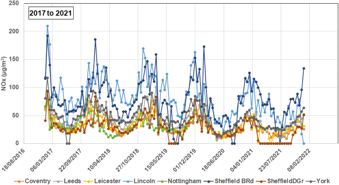Fig. 1 15 days rolling averages of hourly NOx air quality data recorded at eight city sites in Central England between 2017 and 2021. These are raw data trends including periods where no data was recorded (data gaps). See Appendix A for annual displays of this data. The trends identify lower NOx peaks in 2020 and 2021 compared to 2017 to 2019.

Fig. 2 displays the full hourly recorded NOx data together with the 15 days rolling averages for two representative sites: Coventry Allesley (urban background) and Lincoln Canwick Road (urban traffic). These graphs highlight the short-lived nature of high-magnitude NOx concentration spikes at both types of locations, with most high-magnitude spikes occurring in the winter months. At both sites displayed in Fig. 2, the magnitude of the spikes in 2021 is substantially lower than those recorded in 2017 to 2020. This is somewhat surprizing as the most severe COVID-19-driven lockdowns occurred in 2020.

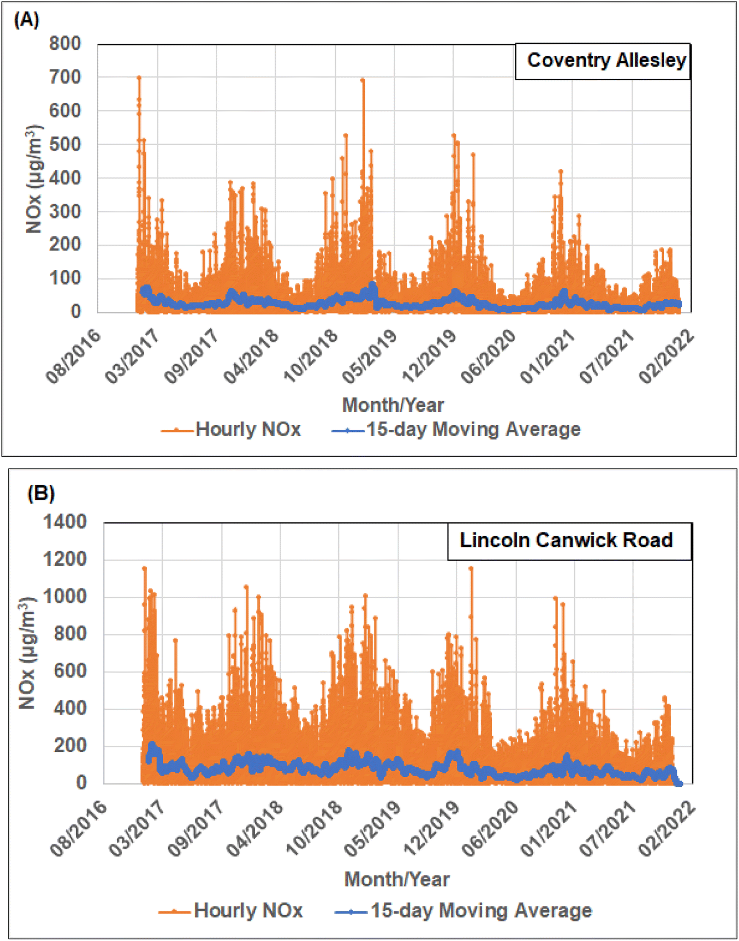Fig. 2 Hourly NOx recorded data at two city sites from Central England from 2017 to 2021: (A) Coventry Allesley (typical of urban background recordings); (B) Lincoln Canwick Road (typical of urban roadside recordings). The trends displayed highlight that both types of recording site display multiple short-lived NOx peaks (spikes) with higher background and peak values occurring at the roadside site.

Fig. 3 plots the percentile values of the NOx hourly recorded data distributions at the Coventry and Lincoln sites for different time intervals in the 2017–2021 period, at both sites, all the percentile values are distinctly higher for the 2017–2019 period. Also, at both sites, all the percentiles up to 80% (displayed as 0.8 in Fig. 2) are slightly higher for 2021 than for 2020. On the other hand, for the percentiles ≥80% the values are higher for 2020 than 2021. This suggests that although the NOx peaks were lower in 2021 than 2020 at both sites, the background NOx values recorded at these sites were lower in 2020 than 2021, which is what would be expected based on the severity of the COVID-19 lockdowns for those two years. These characteristics are representative of the NOx trends at all eight sites studied.

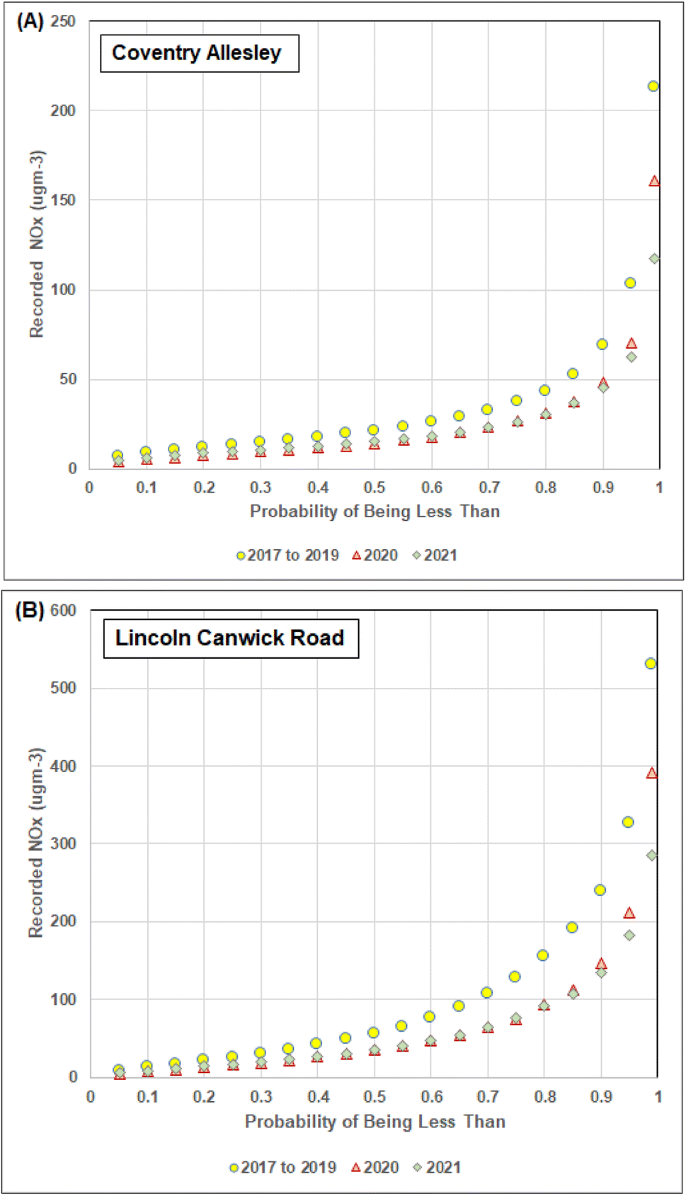Fig. 3 Hourly distributions of NOx air quality measurements for 2017–2019, 2020, and 2021 at two Central England sites: (A) Coventry Allesley (urban background site); and, (B) Lincoln Canwick Road (urban roadside site). The distributions for 2020 and 2021 at both sites display distinctly lower NOx hourly recordings than for 2017 to 2019, particularly at the roadside site.

3. Method

3.1 Trend attributes to characterize NOx hourly records

On an hour-to-hour basis, NOx concentrations at urban sites are strongly influenced by anthropogenic (traffic flow, commercial and industrial) activity, in addition to meteorological and seasonal factors. This makes it very difficult to predict short-term hourly NOx air-quality concentrations in the short term (i.e., the coming few hours) based on hourly recorded meteorological and environmental variables. It is therefore useful to develop and apply univariate prediction methods that rely solely on the information that can be gleaned from the NOx trend recorded in the recent past. A recently developed univariate trend-attribute method has successfully been developed and applied to multi-year hourly ozone concentrations to predict hours-ahead ozone concentrations in city air.²⁷ This approach is adapted in this study to predict hours-ahead NOx concentrations. NOx hourly trends in city air tend to be more spiky than those recorded for ozone because anthropogenic influences have more immediate impacts. This makes univariate hourly prediction analysis more challenging for NOx than for ozone.

The trend-attribute method captures information from the previous twelve hours (t − 12 to t − 1) of the univariate NOx recorded concentrations. It then appends that information as specific trend attributes to the current hour (t0) recorded NOx value. In an hours-ahead prediction configuration, the calculated trend attributes become the independent variables used in a supervised learning context to initially predict the hourly NOx t0 values across a year or multiple years. Due to annual fluctuations in climatic, environmental, and anthropogenic inputs to NOx trends, it is necessary to understand NOx trends at specific city locations in a multi-year context. Once the t0 prediction models are trained validated and tested on a multi-year basis, it is relatively straightforward to adapt them to predict further ahead using the t − 1 to t − 12 independent variables for supervision. In this study, models are developed to predict NOx hours t0, t + 1 (two hours ahead of the available recorded information), and t + 3 (four hours ahead of the available recorded information).

Fifteen trend attributes are calculated for the hourly data compiled for each of the eight city sites. These attributes are defined in Table 2, with the abbreviation used for each attribute displayed in column 1 of that table, and the source or calculation method included in the other columns.

Table 2 Trend-attributes calculated from the univariate NOx air-quality trend recorded from the previous twelve hours (t − 12 to t − 1). These are the variables used as inputs for the NOx prediction models

Variable reference	Attributes extracted from hourly oxides of nitrogen (NOx)	Attribute source/calculation
S	Seasonal component	S calculated by Statsmodel
SD	Derivative of seasonal component (t − 12 to t − 1)	(S(t − 1) less S(t − 12))/11
NOx (t − 1)	NOx for period (t − 1)	Measured NOx for hour t − 1
NOx (t − 2)	NOx for period (t − 2)	Measured NOx for hour t − 2
NOx (t − 3)	NOx for period (t − 3)	Measured NOx for hour t − 3
ANOx(−1 to −3)	NOx average (t − 1) to (t − 3)	Sum NOx (t − 1 : t − 3)/3
ANOx(−1 to −6)	NOx average (t − 1) to (t − 6)	Sum NOx (t − 1 : t − 6)/6
ANOx(−1 to −12)	NOx average (t − 1) to (t − 12)	Sum NOx (t − 1 : t − 12)/12
DNOx(−2 to −1)	NOx difference (t − 2) to (t − 1)	NOx (t − 2) less NOx (t − 1)
DNOx(−3 to −1)	NOx difference (t − 3) to (t − 1)	NOx (t − 3) less NOx (t − 1)
DNOx(−6 to −1)	NOx difference (t − 6) to (t − 1)	NOx (t − 6) less NOx (t − 1)
DNOx(−12 to −1)	NOx difference (t − 12) to (t − 1)	NOx (t − 12) less NOx (t − 1)
RNOx(−3 to −1)	Rate of change NOx (t − 3) to (t − 1)	(NOx (t − 3) less NOx (t − 1))/2
RNOx(−5 to −1)	Rate of change NOx (t − 5) to (t − 1)	(NOx (t − 5) less NOx (t − 1))/4
RNOx(−8 to −1)	Rate of change NOx (t − 8) to (t − 1)	(NOx (t − 8) less NOx (t − 1))/7

---

Attributes S and SD (Table 1) capture hourly information relating to the seasonality fluctuation of the NOx hourly trends. S is extracted from the time series using the Statsmodel seasonal decompose Python-coded function.²⁹ SD then calculates the change/hour of S between t − 12 and t − 1. Fig. 4 displays the hourly SD NOx values associated with the Coventry and Lincoln sites, which are representative of the urban-background and urban-traffic sites studied, respectively. The scale range for Lincoln (Fig. 4B) is three times greater than for Coventry (Fig. 4A), but the relative difference between summer and winter SD values is greater for the urban background than the urban traffic site. This is consistent with greater influence of environmental and climatic contributions to the urban background site, compared to greater anthropogenic contributions, in the form of vehicle emissions, at the urban traffic site.

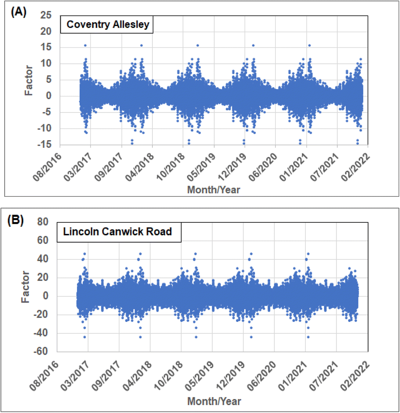Fig. 4 Seasonal derivative (t − 12 to t − 1) (SD) calculated from hourly NOx air quality datasets from 2017 to 2021 for two example recording stations in Central England Cities: (A) Coventry Allesley (urban background site); and, (B) Lincoln Canwick Road (urban roadside site). This trend-attribute variable captures a dimension of seasonality that can be used effectively by the NOx prediction models.

Three trend attributes consider hourly NOx values from the three hours (t − 1 to t − 3) before t0. The other attributes are calculated by applying simple mathematical averages, differences, and rates between recorded NOx concentrations at specific hourly intervals in the range of t − 12 to t − 1.

Other trend attributes could be calculated from the recorded hourly NOx datasets. However, the objective of this study is to demonstrate the value of the trend-attribute method for short-term hours ahead NOx predictions using relatively simple and easy-to-calculate attributes from a limited prior hour interval (t − 12 to t − 1). Future studies are planned to evaluate the influence of other attributes and longer prior-hour intervals (t − 24 to t − 1; t − 36 to t − 1) on NOx hour-ahead prediction accuracy.

3.2 Prediction models applied to hourly trend-attribute NOx datasets

The results of four prediction models applied to the trend-attribute configured hourly NOx air quality concentration datasets are reported in this study. The models are multi-linear regression (MLR), K-nearest neighbour (KNN), support vector regression (SVR) and extreme-gradient boosting (XGB). Several other widely used machine learning methods were also trialled with the datasets, including adaptive boosting, decision tree, extreme-learning machine, multi-layer perceptron neural network, and random forest. However, those models did not improve upon the range of predictions generated by the MLR, KNN, SVR and XGB models and existed with customized Python-coded SciKit Learn functions.³⁰

Regression-based prediction models assume linear relationships between N independent (X_N) and the dependent variable (Y).³¹ They also commonly minimize errors by applying a least-squares-fit method. Various multi-linear regression (MLR) models are available applying simple or more complex error-minimization routines and/or error-penalty functions with or without regularization terms.³¹ The MLR model applied in this study uses a simple least-squares optimization. More complex MLR models such as Ridge, Lasso and ElasticNet were trialled with the compiled NOx dataset but did not improve upon the prediction accuracy obtained by the basic MLR model.

KNN is a data-matching algorithm that, based on combined differences between the independent variable values, establishes the closest matching (nearest neighbour) data records to the data record being predicted.³² SVR establishes optimum-support vectors by translating the variables into multi-dimensional hyperspace.³³ This study applies SVR with a radial basis function (RBF) kernel suitable for datasets with multiple non-linear relationships.³⁴ XGB employs an ensemble of decision trees that it optimizes with a gradient-boosting function.³⁵

The MLR model involved no dataset-specific control parameters to be tuned. However, the three ML models considered do require control parameter tuning and the tuned control parameters applied are listed in Table 3. These control parameter values were determined by trial-and-error tests, the grid-search technique, and/or a Bayesian optimization approach in the case of others.^36,37 The appropriate percentage splits of data records between training and validation subsets used for all four prediction models were determined by the multi-k-fold cross-validation method.³⁸ This was conducted by applying the MLR model to each city dataset incorporating all hourly data records for 2020 and 2021 in separate analyses for those two years. Using appropriate percentage splits helps to improve prediction accuracy, reduce the standard deviations of predictions made by multiple random data selections, and minimize the effects of model overfitting.

Table 3 Control-parameter values applied to the machine learning methods used to predict hourly recorded NOx air quality values for the short-term hours ahead (t0 to t + 3) from 2017 to 2021 in eight cities from central England based on trend attributes. These values are optimized to suit the datasets evaluated

Regression/machine learning algorithms	Algorithm hyperparameter values applied
K Nearest Neighbour (KNN)	Neighbours considered (K) = 15; weighted by Manhattan distance (p = 1)
Linear Regression (LR)	None
Support Vector Regression (SVR)	Kernel = rbf; C = 1100; gamma = 0.5; epsilon = 0.001
Extreme Gradient Boosting (XGB)	Number of estimators = 2000; maximum depth = 10; eta = 0.01; subsample = 0.7; columns sampled per tree = 0.8

---

3.3 Data pre-processing

Data-recording gaps are characteristic of most hourly recorded air quality datasets that prediction models need to contend with. The “hours available” documented for each period of recorded data at each of the eight city sites studied are listed in Table 1 and exclude the data gaps (i.e., all hours for which valid NOx data was not recorded). At some city sites the data gaps are spread relatively evenly across 2017 to 2021, e.g., Coventry Allesley (Fig. 5A), whereas at other locations larger data gaps occur in specific years, e.g., Lincoln Canwick Road (Fig. 5B). However, the data gaps at the city sites selected represent a small percentage of the total 43 824 hours covered from 2017 to 2021, i.e., for the Coventry and Lincoln sites the missing NOx recorded hours represent 2.51% and 2.55% of the total hours respectively. The city sites most impacted by NOx data gaps are the two in Sheffield, with the Barnsley Road site suffering 9.84% data gaps and the Devonshire Green site suffering 18.26% data gaps. However, as the results presented will show, the NOx prediction accuracy achieved at those sites is not unduly impaired by such data gaps.

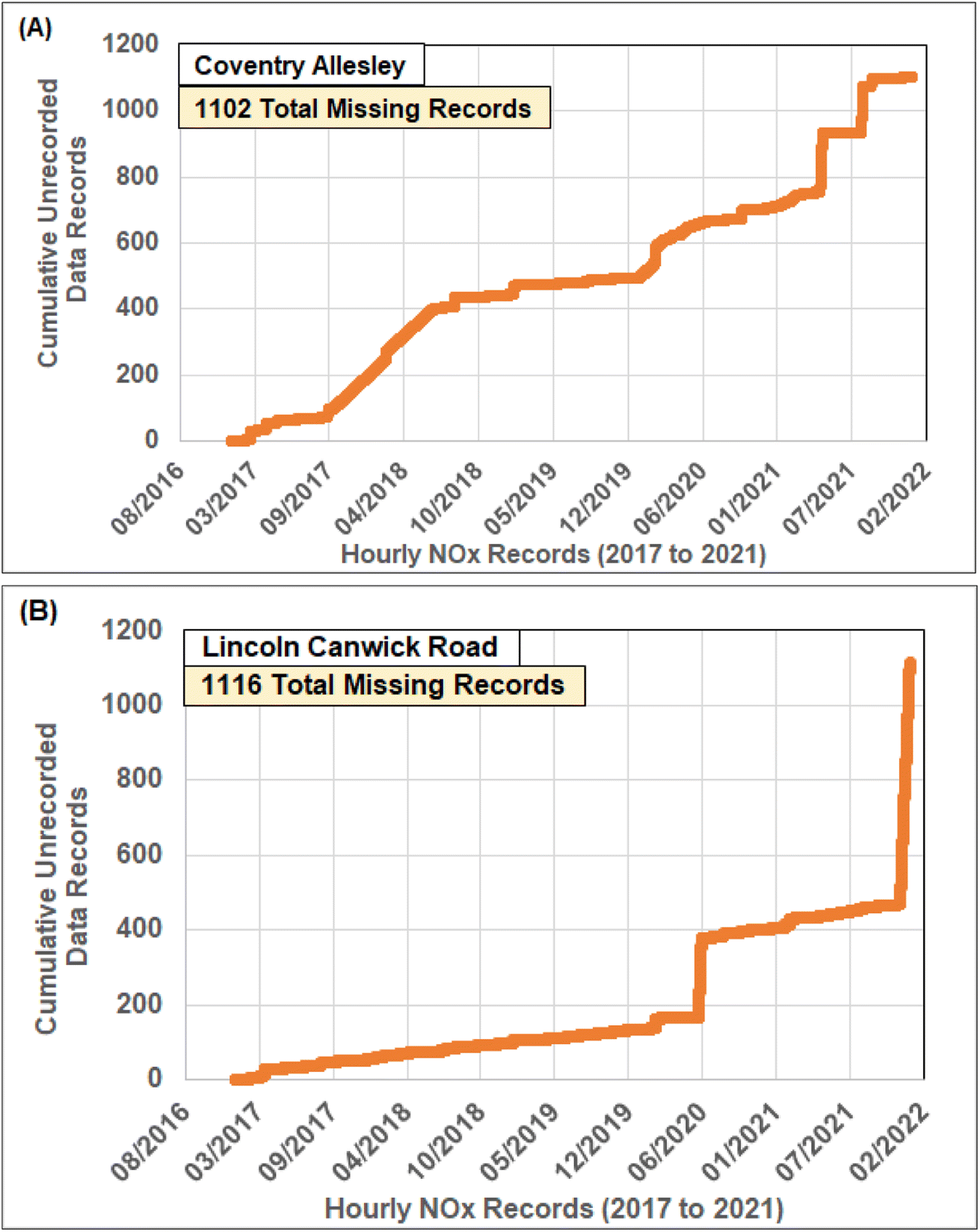Fig. 5 Data gaps in recorded hourly NOx air quality data from 2017 to 2021 for two example recording stations in Central England Cities: (A) Coventry Allesley (urban background site); and, (B) Lincoln Canwick Road (urban roadside site). The time period evaluated involves about 2.5% data gaps at both sites but those gaps are more evenly spread for the Coventry site compared with the Lincoln site.

There are alternative methods for dealing with such data gaps. For some analysis, it is appropriate to fill those gaps with mean or rolling average NOx values for a specified number of prior hours. However, replacing missing values with such estimates is likely to unduly smooth the data trends, so that approach was not adopted. For this prediction study, all missing data periods were excluded from the data sets evaluated by the prediction models. Moreover, as the trend attributes are derived from the prior twelve hours of recorded NOx data, for any hour of missing data the following twelve hours also have to be removed from the dataset to ensure that each data record modelled has the attributed calculated from the correct t − 12 to t − 1 data period. Hence, pre-processing of the datasets required identifying and removing the data gaps and filtering out those data records missing the full t − 12 to t − 1 associated data records.

Each filtered city-site dataset is then configured, in relation to its dependent variable (NOx) in three ways so the t − 12 to t − 1 attributes are assigned to: (1) the t0 NOx recorded values; (2) the t + 1 NOx recorded values; and, (3) the t + 3 NOx recorded values. Datasets of type (1) are modelled to predict NOx t0, whereas datasets of type (2) and (3) are modelled to predict NOx t + 1 and NOx t + 3 as the dependent variable, respectively.

The dataset variables from 2017 to 2021 are all normalized (eqn (1)) prior to prediction modelling to value ranges from −1 to +1. This normalization is necessary to avoid introducing any variable-related scaling biases into the models.

where X_i is the i^th data point within the variable X distribution to be normalized. X_min, X_max and are the minimum, maximum and calculated normalized values relating to the variable X distribution.

3.4 Statistical measures of prediction error monitored

Three commonly used statistical metrics were calculated to assess hourly MLR prediction errors. These metrics are:

Root mean squared error

where X_i = recorded NOx value for data record i; Y_i = predicted NOx value for data record i; and, n refers to the number of data records included in the data subset assessed.

Mean absolute error

For some purposes the MAE divided by the NOx value range is used to clarify the context of the MAE magnitude with respect to specific datasets.

Correlation coefficient squared

where X_mean and Y_mean are means of recorded and predicted NOx values, respectively, for the data subset assessed. This is a useful metric for determining the dispersion and offset of predicted versus measured NOx data in relation to an Y = X line passing through the (X = 0, Y = 0) point.

4. Results

4.1 NOx recorded data and calculated trend attribute relationships

Fig. 6 displays, as heat maps, Pearson and Spearman correlation coefficients between each of the trend attributes and recorded NOx for two representative city sites (Fig. 6A Coventry Allesley, urban background; Fig. 6B Lincoln Canwick Road, urban traffic) for time periods t0, t + 1 and t + 3.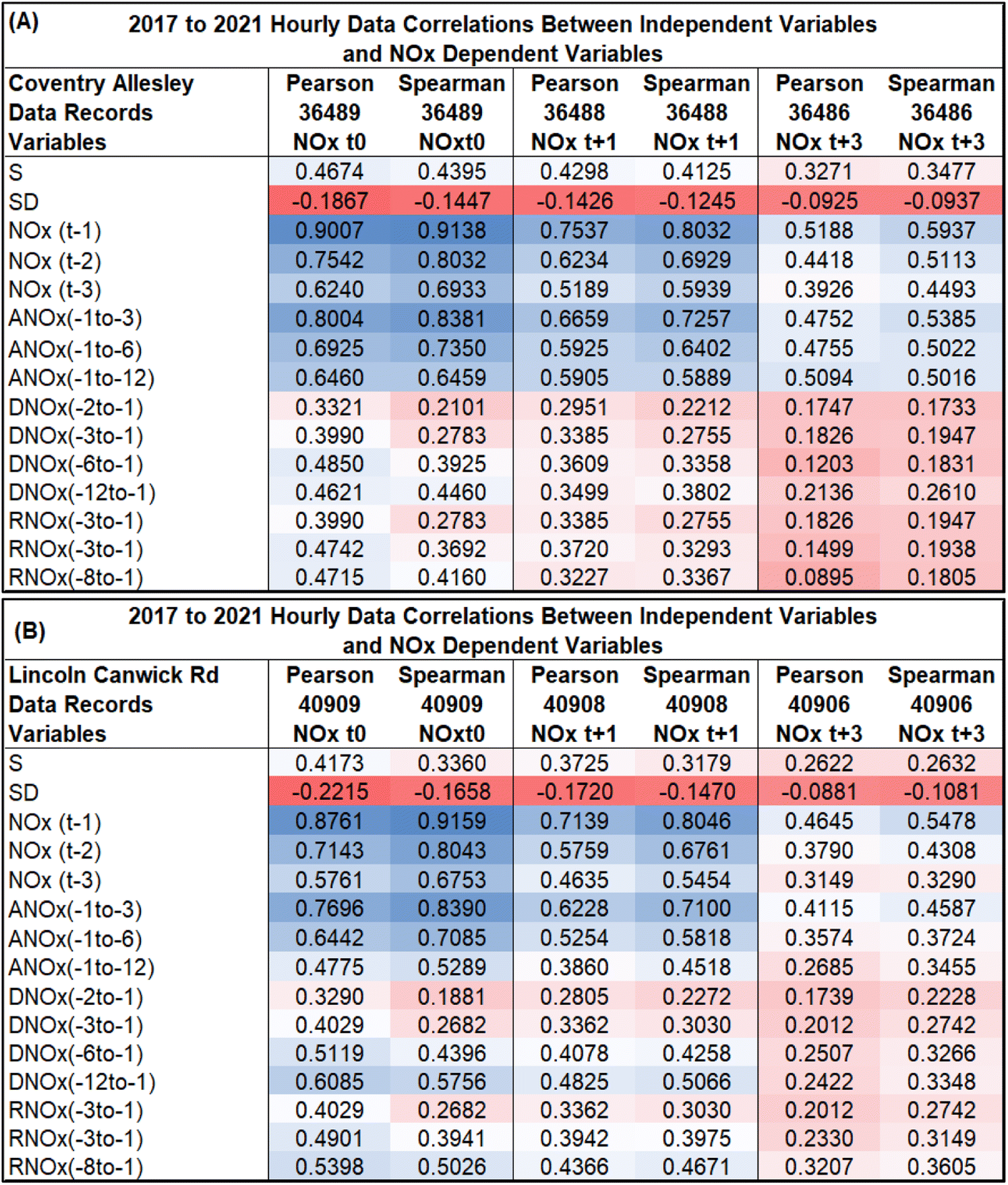

Fig. 6 Heat maps of Pearson (R) and Spearman (p) correlation coefficients between NOx calculated trend attributes and recorded hourly univariate NOx (t0) data, and the same recorded univariate data adjusted to t + 3 hours ahead of the trend attributes: (A) Coventry Allesley (urban background site); and, (B) Lincoln Canwick Road (urban traffic site). Shades of red equate to R and p values from −1 to +0.34, shades of blue equate to R and p values from +0.43 to +1, and R and p values between +0.34 and +0.43 are associated with white to grey background shades. There are poorer correlations between NOx and the attributes for the t + 3 datasets at both sites compared to the t0 and t + 1 datasets.

It is meaningful to compare Pearson and Spearman correlation coefficient values, because the former makes parametric assumptions about the data distributions it compares, whereas the latter does not.³⁹ Where there is good agreement between the two types of correlation coefficient it is indicative that the variable distributions are approximately consistent with parametric assumptions. From Fig. 6 it is apparent that for many of the trend attributes the distribution relationships with recorded NOx value distributions Pearson and Spearman correlation coefficient values are not in close agreement. This suggests that there are non-parametric and, in some cases at least, non-linear relationships between the distributions. The existence of multiple non-parametric relationships between NOx and the influencing variables has an impact on the ability of MLR and ML models to predict those trends.

Comparing Fig. 6A and B reveals that the range of correlation coefficient values between the trend-attribute variables and NOx is quite similar at both sites for each of the periods considered. For time period t0 (1 hour ahead of the closest hourly period for which prior data is available) the highest correlation coefficients occur between NOx t0 and NOx (t − 1), close to 0.9 at both sites. High correlation coefficient values (>0.6) also exist for the period hour t − 2, hour t − 3, and the three average attributes spread over the past twelve hours with NOx t0. Moderate correlation coefficient values (between 0.4 and 0.6) for most of the other attributes with NOx t0. At both sites, the lowest correlation coefficients are between DNOx(−2 to −1) and NOx t0. Higher correlation coefficient values exist between DNOx(−12 to −1) and RNOx(−8 to −1) and NOx t0 at the Lincoln site than at the Coventry site.

The correlation-coefficient values for attributes versus NOx t + 1 show similar relative variations but with slightly lower values than those with NOx t0. The generally high correlation coefficient values between the attributes and NOx t0 and NOx t + 1 suggest that those attributes should be relatively easy for MLR and ML models to exploit in generating relatively accurate NOx predictions for those periods.

The correlation coefficient values between the attributes and NOx t + 3 are substantially lower, in most cases than those recorded for periods NOx t0 and NOx t + 1 and are more evenly valued for attributes covering the entire t − 12 to t − 1 periods. Nevertheless, a substantial number of the attributes display correlation coefficient values with NOx t + 3 with values >0.2 (eight attributes do so for the Coventry site, whereas thirteen attributes do so for the Lincoln site). The roadside site has somewhat higher correlation coefficient values with NOx t + 3 for the attributes involving periods in the t − 12 to t − 6 interval than the urban background site. These relationships suggest that MLR and ML models will find it more difficult to predict NOx t + 3 than NOx t + 1 or NOx t0 from these attributes but are more likely to make more use of the attributes involving periods in the t − 12 to t − 6 interval.

4.2 Multi-K-fold cross-validation analysis

The multi-K-fold cross-validation technique was applied to each city dataset to establish the most suitable random data splits to employ between training and validation data subsets to maximize prediction accuracy and consistency and minimize the risk of overfitting the datasets.³⁸ This involved performing 4-fold, 5-fold, 10-fold, and 15-fold analyses, each repeated three times, and the mean and standard deviation of the MAE and RMSE metrics were calculated for each fold. This analysis was performed with the MLR model because that model involved the shortest execution time and multiple cases needed to be evaluated (e.g., the 15-fold analysis run three times involves 45 runs for each dataset). Two t0-time-period datasets were evaluated for each city site: one involving all the pre-processed available hourly records for 2020; and the other all the hourly records for 2021. Table 4 presents the multi-K-fold cross-validation results.

Table 4 Cross validation results for the eight cities studied using the MLR model to compare different splits of the data between training, validation and testing subsets applied to predict 2020 and 2021 hourly data. RMSE and MAE values are expressed in units of μg m⁻³. All folds evaluated generate comparable prediction accuracy for a specific site but that accuracy varies from site to site

Multi-fold cross validation analysis applying the MLR algorithm to hourly NOx air-quality data recorded at eight city sites from Central England
NOx recording station	Cross-fold validation	2020 (t0)				2021 (t0)
		MAE		RMSE		MAE		RMSE
		Mean	St.Dev	Mean	St.Dev	Mean	St.Dev	Mean	St.Dev
Coventry Allesley	4-fold (75 : 25)	5.32	0.11	10.21	0.44	6.41	0.20	12.12	0.68
	5-fold (80 : 20)	5.31	0.14	10.20	0.54	6.42	0.20	12.13	0.82
	10-fold (90 : 10)	5.31	0.27	10.16	0.94	6.41	0.26	12.08	1.22
	15-fold (∼93 : ∼7)	5.30	0.37	10.10	1.45	6.42	0.36	12.06	1.48
Leeds Centre	4-fold (75 : 25)	6.90	0.20	12.10	0.73	7.55	0.27	13.43	1.04
	5-fold (80 : 20)	6.90	0.19	12.10	0.70	7.54	0.31	13.43	1.04
	10-fold (90 : 10)	6.90	0.33	12.07	1.11	7.53	0.38	13.40	1.34
	15-fold (∼93 : ∼7)	6.90	0.45	12.03	1.46	7.53	0.46	13.36	1.55
Leicester University	4-fold (75 : 25)	7.17	0.18	12.73	0.73	7.17	0.21	12.00	0.84
	5-fold (80 : 20)	7.16	0.25	12.71	1.13	7.16	0.23	12.01	0.73
	10-fold (90 : 10)	7.15	0.33	12.65	1.39	7.16	0.42	11.96	1.25
	15-fold (∼93 : ∼7)	7.15	0.43	12.60	1.71	7.16	0.46	11.93	1.49
Lincoln Canwick Road	4-fold (75 : 25)	20.34	0.34	36.14	0.98	18.20	0.43	29.24	0.68
	5-fold (80 : 20)	20.36	0.53	36.15	1.63	18.20	0.37	29.24	0.87
	10-fold (90 : 10)	20.34	0.88	36.06	2.89	18.19	0.71	29.21	1.59
	15-fold (∼93 : ∼7)	20.33	1.07	36.01	3.31	18.19	0.84	29.18	2.01
Nottingham Centre	4-fold (75 : 25)	6.37	0.21	12.40	1.28	7.08	0.18	13.35	0.64
	5-fold (80 : 20)	6.36	0.19	12.33	1.36	7.07	0.20	13.35	0.65
	10-fold (90 : 10)	6.34	0.34	12.21	2.07	7.06	0.30	13.30	1.16
	15-fold (∼93 : ∼7)	6.34	0.44	12.18	2.36	7.06	0.46	13.18	1.96
Sheffield Barnsley Road	4-fold (75 : 25)	19.43	0.36	31.70	1.17	21.77	0.55	34.16	1.44
	5-fold (80 : 20)	19.43	0.48	31.68	1.30	21.78	0.48	34.19	1.43
	10-fold (90 : 10)	19.42	0.63	31.62	2.24	21.76	0.76	34.12	2.12
	15-fold (∼93 : ∼7)	19.41	0.91	31.57	2.92	21.76	1.01	34.09	2.55
Sheffield Devonshire Green	4-fold (75 : 25)	7.69	0.25	16.93	1.43	9.41	0.33	20.89	2.95
	5-fold (80 : 20)	7.70	0.32	16.96	1.62	9.41	0.56	20.81	3.32
	10-fold (90 : 10)	7.68	0.46	16.83	2.40	9.40	0.89	20.50	4.85
	15-fold (∼93 : ∼7)	7.67	0.54	16.74	2.74	9.38	1.07	20.30	5.58
York Fishergate	4-fold (75 : 25)	10.04	0.23	16.74	0.69	9.81	0.26	16.22	0.60
	5-fold (80 : 20)	10.02	0.37	16.71	0.75	9.81	0.32	16.22	0.75
	10-fold (90 : 10)	10.02	0.51	16.68	1.21	9.81	0.46	16.18	1.27
	15-fold (∼93 : ∼7)	10.02	0.58	16.65	1.54	9.80	0.55	16.16	1.48

---

It is apparent from Table 4 that the MLR models generate distinctive prediction errors for each city dataset for 2020 and 2021. As to be expected, the roadside sites (Lincoln Canwick Road, Sheffield Barnsley Road, and York Fishergate) generate higher mean prediction errors than the urban background sites. However, the range of prediction-error standard deviations of error is similar for all city sites. All folds studied generate credible and comparable prediction results for specific sites, with the 15-fold analysis generating the highest standard deviations of errors for each specific city site, and the 4-fold analysis the lowest standard deviations of errors.

Fig. 7 displays RMSE versus MAE the MLR multi-K-fold analysis results, with each city plotting in distinct positions for 2020 (Fig. 7A) and 2021 (Fig. 7B). At the scale displayed all four K-fold values for a specific city overlie each other in Fig. 7. This suggests that random dataset splits between 75% : 25% and 93% : 7% (training : testing) should all provide similar mean NOx t0 prediction results, with the 75% : 25% and 80% : 20% splits generating the lowest error standard deviations. Based on these results, 80% : 20% splits were used for the random sampling MLR and ML modelling conducted for this study.

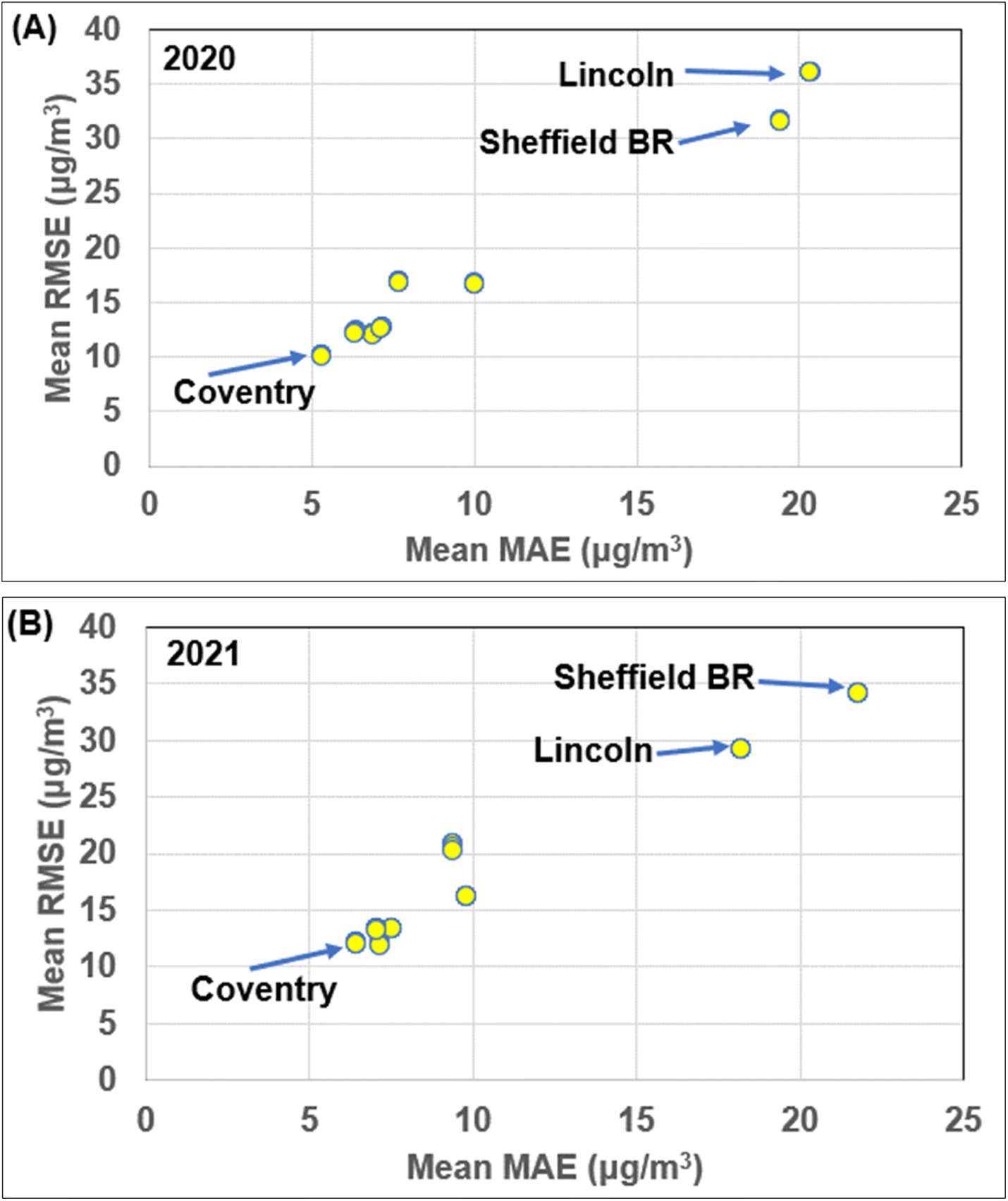Fig. 7 Multi-fold cross validation errors for the MLR model applied to the NOx air-quality hourly data for eight cities from Central England for: (A) 2020; and (B) 2021. The mean prediction error (RMSE and MAE) results for 4-fold, 5-fold, 10-fold and 15-fold cross-validation analysis presented in Table 4 are all displayed and in almost all cases overlie each other for the dataset recorded at specific cities. The Lincoln and Sheffield BR roadside recording sites generate substantially higher NOx prediction errors than the other sites.

4.3 Training, validation and testing results for four NOx t0 prediction models

The MLR, KNN, SVR and XGB models were each applied to predict hourly NOx t0 for 2020 datasets for each of the city sites (testing subset) based on models trained and validated using hourly NOx t0 for 2017 to 2019. The results are displayed in Table 5.

Table 5 Hourly NOx air quality prediction performances of four supervised machine learning models trained and validated with 2017 to 2019 data to predict the testing subset comprising of the 2020 data. The models are applied to the datasets from eight cities in Central England. Model execution times (seconds) are also provided. The results reveal that the SVR and XGB models outperform the MLR and KNN models in their 2020 predictions for each site^a

Oxides of nitrogen univariate hourly predictions for period t0 based on fifteen attributes calculated from preceding periods t − 1 to t − 12
NOx recording station	Machine learning algorithm	Period 2017 to 2019			Period 2017 to 2019			Period 2020			Execution
		Training subset (80%)			Validation subset (20%)			Testing subset (100%)			Time
		RMSE	MAE	R ^2	RMSE	MAE	R ^2	RMSE	MAE	R ^2	Seconds
a (1) RMSE and MAE values are expressed in units of μg m^−3; (2) MLR and KNN execution times include 5-fold cross-validation, SVR and XGB execution times do not.
Coventry Allesley	MLR	16.39	8.55	0.84	15.89	8.81	0.88	10.31	5.71	0.82	6.10
	KNN	0.00	0.00	1.00	17.09	8.32	0.85	9.60	5.29	0.84	56.46
	SVR	13.44	7.04	0.89	15.13	7.81	0.89	9.14	4.70	0.86	279.07
	XGB	2.96	2.13	0.99	14.94	7.87	0.89	9.23	5.04	0.85	90.10
Leeds Centre	MLR	18.48	10.79	0.83	21.90	11.39	0.81	13.16	8.48	0.80	5.99
	KNN	0.00	0.00	1.00	19.86	10.58	0.82	12.15	7.59	0.83	77.84
	SVR	15.31	9.19	0.88	18.43	10.01	0.86	11.12	6.52	0.86	383.73
	XGB	4.40	3.25	0.99	17.88	9.97	0.85	11.50	6.87	0.85	116.00
Leicester University	MLR	16.65	9.20	0.80	16.95	9.25	0.82	12.84	7.64	0.82	6.06
	KNN	0.00	0.00	1.00	15.48	8.72	0.84	12.02	7.11	0.85	74.35
	SVR	11.38	6.25	0.86	15.45	8.10	0.85	11.38	6.25	0.86	354.23
	XGB	3.65	2.65	0.99	15.08	8.31	0.84	11.88	6.66	0.85	127.72
Lincoln Canwick Road	MLR	50.36	30.54	0.80	50.46	30.34	0.80	37.97	24.63	0.77	12.49
	KNN	0.00	0.00	1.00	47.32	25.94	0.82	34.30	19.20	0.81	65.47
	SVR	41.61	23.18	0.86	46.86	24.72	0.83	31.15	17.55	0.85	348.82
	XGB	11.67	8.39	0.99	46.01	24.62	0.83	32.61	18.38	0.83	127.15
Nottingham Centre	MLR	18.70	10.24	0.81	21.18	10.34	0.77	12.70	7.24	0.84	6.38
	KNN	0.00	0.00	1.00	19.12	9.82	0.81	12.48	6.98	0.84	76.92
	SVR	16.23	8.92	0.86	15.34	8.94	0.88	12.05	6.01	0.85	347.95
	XGB	4.34	3.19	0.99	17.79	9.52	0.83	12.09	6.48	0.85	106.99
Sheffield Barnsley Road	MLR	40.86	25.00	0.80	41.01	25.56	0.79	31.71	19.62	0.81	5.97
	KNN	0.00	0.00	1.00	38.84	23.06	0.81	30.80	18.78	0.82	89.28
	SVR	34.93	20.86	0.85	39.36	22.68	0.80	28.46	16.99	0.85	315.67
	XGB	9.69	7.13	0.99	37.73	22.48	0.82	29.52	17.83	0.84	119.08
Sheffield Devonshire Green	MLR	19.13	9.41	0.82	23.01	9.76	0.76	17.10	8.06	0.79	5.84
	KNN	0.00	0.00	1.00	21.07	9.02	0.78	16.38	7.44	0.80	68.95
	SVR	15.87	7.83	0.88	18.16	8.24	0.85	14.96	6.53	0.84	310.16
	XGB	3.60	2.59	0.99	17.71	8.28	0.85	15.12	6.82	0.83	99.78
York Fishergate	MLR	24.73	15.73	0.79	24.84	15.58	0.80	18.22	12.64	0.75	6.82
	KNN	0.00	0.00	1.00	22.44	13.73	0.82	16.46	10.89	0.80	62.17
	SVR	20.78	12.70	0.85	22.08	13.24	0.84	15.17	9.33	0.83	267.54
	XGB	5.39	3.96	0.99	21.42	13.19	0.84	15.75	9.88	0.82	103.12

---

From Table 5 results for the training, validation, and testing subsets, it is apparent that the SVR and XGB models generate fewer NOx t0 prediction errors (MAE and RMSE) than the MLR and KNN models for all eight city sites. Although the MLR and KNN models provide consistent NOx to prediction results for 2020, trained and validated with 2017–2019 hourly data, and are executed relatively rapidly for these data subsets (MLR in about 6 to 13 seconds; KNN in about 57 to 90 seconds) their prediction capabilities are inferior to the SVR and XGB models.

For the eight cities evaluated the SVR and XGB models generated quite similar NOx t0 prediction results for 2020 (Table 5) based on models trained with 2017–2019 hourly data. However, in the case of all cities, the MAE and RMSE values for the 2020 subset are slightly lower for the SVR model. However, with these relatively large datasets, the SVR models involve substantially longer execution times (about 268 to 384 seconds) to perform the training, validation, and testing than the XGB models (about 90 to 128 seconds).

The relative values of the MAE and RMSE NOx t0 (2020) prediction errors generated for each of the cities by the MLR and ML models are consistent with the K-fold cross-validation results, as shown by a comparison of the Table 5 results with the error values displayed in Fig. 7. As expected, the roadside recording sites (Lincoln Canwick Road and Sheffield Barnsley Road) generate substantially higher NOx t0 (2020) errors than the other city sites. The Table 5 results justify the preferential application of the SVR and XGB models to conduct hourly NOx predictions using subsets covering various periods within the 2017 to 2021 compiled dataset.

4.4 NOx t0 predictions for 2020 and 2021 from different training periods

Table 6 displays the prediction error results for the SVR and XGB models trained and validated with hourly data from different periods to predict testing subsets for 2020 and 2021. The 2020 predictions are made separately with models trained and validated with a 2017–19 subset (already shown in Table 5) and with a 2021 subset. The 2021 predictions are made separately with models trained and validated with a 2017–20 subset and with a 2020 subset. For most cities, the models trained and validated with data from multiple years generate slightly lower prediction errors than for models trained with data from single years. This justifies the use of multi-year data subsets for model training and validation.

Table 6 Hourly NOx prediction results for 2020 and 2021 using different training periods for the SVR and XGB machine-learning models for the eight cites evaluated from Central England. For most cities, ML models trained with the longer time periods generate just slightly lower prediction errors than those models trained with data from just one year. The results reveal that the models trained with data from multiple years generate slightly more accurate predictions than models trained with data from a single year^a

Oxides of nitrogen univariate hourly predictions for period t0 using different training and testing periods based on fifteen attributes calculated from preceding periods t − 1 to t − 12
NOx recording station	Machine learning algorithm	2017_19 trained model		2021 trained model		2017_20 trained model		2020 trained model		Execution times^b (seconds)
		Predict 2020 (100%)		Predict 2020 (100%)		Predict 2021 (100%)		Predict 2021 (100%)
		RMSE	MAE	RMSE	MAE	RMSE	MAE	RMSE	MAE
a RMSE and MAE values are in units of μg m^−3. b Execution time refers to the 2020 trained/validated model (∼8000 hourly records) applied to predict the 2021 subset (∼8000 hourly records).
Coventry Allesley	SVR	9.14	4.70	9.33	4.71	12.05	5.81	11.95	6.02	31.42
	XGB	9.23	5.04	9.52	4.97	11.86	6.03	12.27	6.16	28.63
Leeds Centre	SVR	11.12	6.52	11.46	6.40	13.13	7.32	14.32	7.43	49.82
	XGB	11.50	6.87	12.07	6.72	13.27	7.51	14.33	7.62	48.81
Leicester University	SVR	11.38	6.25	12.03	6.42	11.62	6.60	12.69	7.00	47.79
	XGB	11.88	6.66	12.79	6.95	11.68	6.86	12.84	7.20	39.37
Lincoln Canwick Road	SVR	31.15	17.55	38.67	18.16	27.05	16.67	27.80	16.73	49.69
	XGB	32.61	18.38	38.24	18.81	27.56	17.12	28.08	17.15	43.98
Nottingham Centre	SVR	12.05	6.01	13.77	5.95	12.76	6.59	13.84	6.76	53.40
	XGB	12.09	6.48	14.39	6.43	13.08	6.90	14.39	7.04	40.14
Sheffield Barnsley Road	SVR	28.46	16.99	30.72	17.72	33.12	20.24	35.53	21.16	31.21
	XGB	29.52	17.83	31.92	18.49	33.42	20.37	35.63	21.38	35.53
Sheffield Devonshire Green	SVR	14.96	6.53	21.08	7.49	22.05	8.97	22.71	9.23	48.51
	XGB	15.12	6.82	21.03	7.93	22.17	9.28	21.15	9.26	36.04
York Fishergate	SVR	15.17	9.33	16.13	8.98	15.57	9.28	17.10	9.45	45.23
	XGB	15.75	9.88	16.42	9.34	15.88	9.61	16.92	9.57	36.50

---

4.5 NOx prediction results looking further forward to hours t + 1 and t + 3

Although SVR provides marginally lower NOx prediction errors than XGB, the results of the two models are consistent and comparable when plotted on scales able to display the prediction errors associated with all eight city sites studied. The analysis presented for predicting NOx t + 1 and NOx t + 3 data for 2020 and 2021 using models trained hours from several previous years is displayed for the XGB model. The XGB model is selected in preference to the SVR model for this purpose for two reasons: (1) it executes substantially more quickly than the SVR model for trained and validating multi-year, hourly data; and (2) because it more readily yields information relating to the relative influence of each trend attribute on the solutions it generates.

Table 7 and Fig. 8 display the results for the XGB models applied to predict NOx t + 1 and NOx t + 3. Except for the Leicester University site, all the other sites generate higher prediction errors for NOx t + 1 (2020) compared to NOx t0 (2020). The 2020 prediction errors are substantially higher for the two roadside NOx recording sites for the t + 1 versus t0 predictions compared to the other sites. This is also the case for the 2021 t + 1 predictions. For each city, the NOx t + 3 predictions are associated with substantially higher prediction errors for 2020 and 2021 datasets compared to the NOx t + 1 predictions, particularly for two of the two roadside recording stations (Fig. 8).

Table 7 Hourly NOx prediction results for periods t + 1 and t + 3 applying the XGB machine learning models applied to the 2020 and 2021 datasets for the eight cites evaluated from Central England. XGB is applied in preference to SVR because it executes more quickly when trained with large datasets and reveals the relative influence of each trend attribute on the optimum solutions. The results highlight the somewhat inferior prediction accuracy of the t + 3 datasets particularly in terms of R² due to many peak values being underestimated^a

Oxides of nitrogen univariate hourly predictions from period t + 1 and t + 3 fifteen attributes from periods t − 1 to t − 12
NOx recording station	Machine learning algorithm	Trained model 2017–19					Trained model 2017–20					Execution time (seconds)
		NOx range	2020 test subset (100%)				NOx range	2021 test subset (100%)
			RMSE	MAE	R ^2	MAE/range		RMSE	MAE	R ^2	MAE/range
a (1) RMSE and MAE values are in units of μg m^−3; (2) XGB execution times are for 2017_2020 training and testing 2021 hourly data. It excludes 5-fold cross-validation.
NOx predicted hourly period for t + 1
Coventry	XGB	419.53	18.02	9.36	0.67	2.2%	284.24	16.11	8.77	0.48	3.1%	145.74
Leeds	XGB	400.08	18.03	11.33	0.62	2.8%	419.60	19.39	11.43	0.57	2.7%	168.02
Leicester	XGB	389.47	9.33	5.47	0.91	1.4%	377.13	17.17	10.30	0.61	2.7%	161.41
Lincoln	XGB	1148.91	49.38	28.19	0.61	2.5%	517.36	39.59	25.01	0.58	4.8%	150.69
Nottingham	XGB	660.47	18.04	10.09	0.67	1.5%	511.11	17.77	9.89	0.62	1.9%	142.61
Sheffield B Rd	XGB	777.17	43.75	26.97	0.64	3.5%	670.00	46.15	29.24	0.54	4.4%	146.86
Sheffield DG	XGB	656.62	23.65	11.09	0.59	1.7%	476.55	30.67	13.55	0.38	2.8%	149.10
York	XGB	443.48	23.66	15.51	0.58	3.5%	394.79	22.67	14.31	0.54	3.6%	139.34
NOx predicted hourly for period t + 3
Coventry	XGB	419.53	24.58	13.85	0.38	3.3%	284.24	20.35	12.48	0.16	4.4%	124.21
Leeds	XGB	400.08	25.74	17.21	0.24	4.3%	419.60	25.78	16.11	0.23	3.8%	171.61
Leicester	XGB	389.47	24.91	15.72	0.34	4.0%	377.13	22.85	14.54	0.31	3.9%	152.93
Lincoln	XGB	1148.91	66.47	42.37	0.30	3.7%	517.36	53.29	36.64	0.24	7.1%	149.66
Nottingham	XGB	660.47	24.67	14.81	0.39	2.2%	511.11	22.78	13.64	0.38	2.7%	137.96
Sheffield B Rd	XGB	777.17	58.58	38.83	0.36	5.0%	670.00	59.31	39.38	0.25	5.9%	124.76
Sheffield DG	XGB	656.62	31.07	16.18	0.30	2.5%	476.55	35.59	18.75	0.15	3.9%	143.81
York	XGB	443.48	32.02	22.89	0.24	5.2%	394.79	29.41	19.52	0.23	4.9%	144.25

---

Fig. 8 Hourly NOx air quality prediction errors generated by XGB models applied to periods t0, t + 1, and t + 3 compared for eight cities from Central England for (A) 2020 predicted using a model trained with 2017 to 2019 data; and (B) 2021 predicted using a model trained with 2017 to 2020 data. The urban roadside recording sites (Lincoln Canwick Road and Sheffield Barnsley Road) generate the highest prediction errors for each t0, t + 1, and t + 3. The cities evaluated display similar prediction error relationships for 2020 and 2021.

Despite the increase in errors associated with the NOx t + 1 and NOx t + 3 predictions for the 2020 and 2021 periods compared to those for NOx t0, in the context of the recorded NOx range at each site (Table 7) for those periods the prediction errors remain quite low. This is apparent from the MAE/NOx range ratios displayed in Table 7. For the NOx t + 1 predictions (2020 and 2021) the MAE/range ratio is less than 3% for each city site, apart from Lincoln Canwick Road, Sheffield Barnsley Road, and York Fishergate. The Nottingham Centre site generates the lowest MAE/range ratios (<2%) for its 2020 and 2021 NOx t + 1 predictions. For the NOx t + 3 predictions (2020 and 2021) the MAE/range ratio is substantially less than 5% for each city site, apart from Lincoln Canwick Road, Sheffield Barnsley Road, and York Fishergate. Once again, the Nottingham Centre site records the lowest MAE/range ratios for 2020 and 2021 NOx t + 3 predictions.

These results indicate that the trend attributes calculated from the t − 12 to t − 1 hourly recorded NOx data, can for the majority of hours recorded, provide predictions with meaningful accuracy for short-term forecasts up to t + 3 (four hours ahead of the last available hourly recording). However, it is apparent from Table 7 that the R² values for the t + 3 predictions are very low in comparison with the t0 and t + 1 forecasts. These low R² values are primarily a consequence of the t + 3 model predictions under-estimating the values of many of the NOx recorded peaks, which substantially weakens the correlations between predicted and measured NOx values. This highlights that there is substantial room for improvement concerning the t + 3 period NOx forecasts.

4.6 Relative influence of the trend attributes on the XGB NOx predictions

The XGB algorithm determines the relative importance of each independent variable in the prediction solutions provided by each of the component decision trees it generates. It does this by quantifying the extent to which each variable contributes to the division of data records at each specific decision-tree node. For the NOx hourly prediction models generated, such information usefully distinguishes the extent to which each of the trend attributes contributes to the XGB solutions. These feature importance measures for the Coventry and Lincoln sites are compared in Fig. 9 for the t0, t + 1, and t + 3 predictions made by the trained XGB models for the periods 2017–2019, 2020, and 2021. It is apparent from Fig. 9 that all 15 trend attributes make some contribution to the XGB model NOx prediction solutions for all periods considered.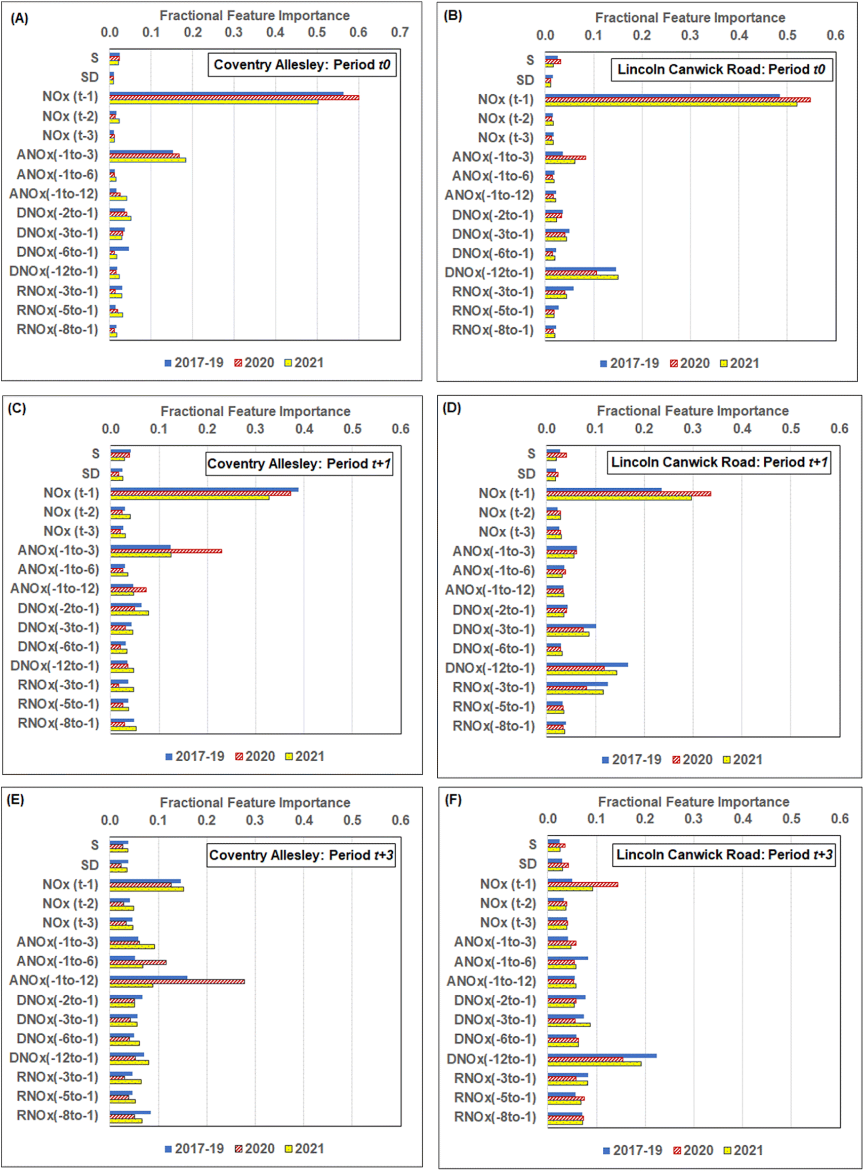

Fig. 9 Fractional feature importance of individual trend attributes to XGB model predictions of NOx air quality for the Coventry Allesley site: (A) t0; (C) t + 1; (E) t + 3; and the Lincoln Canwick Road site: (B) t0; (D) t + 1; (F) t + 3. The models rely on contributions from features to a different extent depending on the periods forecast. Also, the roadside sites exploit the difference and rate of change trend attributes to a greater extent than the urban background sites.

For the NOx t0 predictions at the Coventry site (Fig. 9A), the attribute NOx t − 1 makes the largest fractional contribution (>0.5) to the XGB solution for each time interval considered. The attribute ANOx(−1 to −3) also makes a substantially higher fractional contribution (>0.1) than the other attributes. These two trend attributes also make important contributions to t0 XGB solutions for the Lincoln site (Fig. 9B). However, the second most important attribute (>0.1) for the Lincoln site t0 solutions is DNOx(−12 to −1). These relative influences are consistent with the relative magnitudes of the correlation coefficients between the attributes and NOx t0 at those two sites (Fig. 6).

For the NOx t + 1 predictions at the Coventry (Fig. 9C) and Lincoln (Fig. 9D) sites the attribute NOx t − 1 continues to make the largest fractional contribution (>0.3). At the Coventry site, the ANOx(−1 to −3) attribute continues to make the second highest fractional contribution (>0.1) than the other attributes. On the other hand, at the Lincoln site the attributes the DNOx(−12 to −1), DNOx(−3 to −1) and RNOx(−3 to −1) make higher relative contributions than the ANOx(−1 to −3) attribute to the NOx t + 1 XGB solutions. This relative order of importance of the attributes at the Lincoln site for the XGB NOx t + 1 solutions is not in direct agreement with the correlation coefficients (Fig. 6), as the ANOx(−1 to −3) attribute displays the second highest correlation coefficients with NOx t + 1 at that site.

For the NOx t + 3 predictions ANOx(−1 to −3) attribute represents the second most influential attribute at both sites. At the Coventry site, the attribute ANOx(−1 to −12) is the most important, which is explainable in terms of its correlation coefficients (Fig. 6). On the other hand, at the Lincoln site, the DNOx(−12 to −1) attribute is the most influential for the NOx t + 3 XGB solutions, which is not consistent with the correlation coefficient distributions for that site (Fig. 6).

In broad terms, it is apparent at both sites displayed, and the other studied city sites, that as the predictions move further forward in time from t0 to t + 13, the attributes including information relating to the interval t − 12 to t − 3 make greater relative contributions. This is particularly so for the roadside NOx recording sites.

4.7 Alternative prediction models applied to the NOx air quality datasets

It is appropriate to place the NOx predictions presented based on trend attributes with alternative methods of univariate forecasting methods. For t0 forecasting relatively straightforward methods to apply are the so-called naïve forecast and a rolling average. The naïve forecasts simply take the t − 1 value as the t0 prediction. Rolling averages involving different ranges in the t − 12 to t − 1 available data were tested with the 8-city NOx datasets, the two-period (t − 2 to t − 1) rolling averages generated the lowest moving-average prediction errors of the intervals tested. Naïve and two-period rolling average forecasts are shown for NOx to 2020 and 2021 predictions in Table 8.

Table 8 Naïve and moving average NOx air quality forecasts for period t0 applied to the 2020 and 2021 datasets for the eight cites evaluated from Central England. It is useful to compare this values with the trend-attribute prediction errors for these time periods displayed in Tables 5 and 6

NOx recording station (μg m^−3)	Naïve forecast		2-Period moving average
	RMSE	MAE	RMSE	MAE
	2020 t0		2020 t0
Coventry	14.34	6.33	17.38	7.76
Leeds	13.12	6.97	15.71	8.45
Leicester	14.20	7.19	17.04	8.69
Lincoln	40.13	20.39	47.28	24.24
Nottingham	13.59	6.40	15.93	7.60
Sheffield B Rd	35.26	19.87	41.16	23.56
Sheffield DG	18.17	7.27	20.69	8.62
York	19.24	10.36	22.06	12.19
	2021 t0		2021 t0
Coventry	11.37	5.83	13.50	7.09
Leeds	14.31	7.71	16.76	9.18
Leicester	12.80	7.21	15.04	8.49
Lincoln	31.27	18.39	36.04	21.26
Nottingham	13.90	7.08	15.76	8.26
Sheffield B Rd	37.14	22.42	43.22	26.36
Sheffield DG	22.22	9.34	25.39	10.94
York	17.60	10.11	20.62	11.97

---

The trend-attribute derived NOx t0 2020 and 2021 predictions (Tables 5 and 6) generate substantially lower errors than the two-period rolling average t0 predictions for all of the cities studied. This is also mostly the case for the NOx t0 naïve predictions, except for the Nottingham site for 2020 (for MAE only) and the Coventry site for 2021 (for both MAE and RMSE) for which the naïve forecasts are slightly better than the XGB forecasts. An explanation for this outcome for those two sites is proposed in the Discussion. The naïve forecast and two-period rolling average predictions for NOx t + 1 and t + 3 (not shown) generated substantially higher errors for all periods and all cities compared to the MLR and ML models.

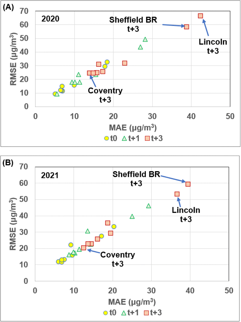
Another alternative short-term prediction method that is widely used to generate forecasts from univariate NOx time series is the ARIMA method.^22,23Table 9 displays the results of an ARIMA(1,0,0) model for the Coventry and Lincoln sites for NOx t0, t + 1, and t + 3 forecasts for 2020 and 2021 compared to the XGB model results. Higher-order ARIMA models with p ≥ 1, d ≥ 0, and q ≥ 1 (p adjusts the autoregressive element, d adjusts the seasonal-differencing element, and q adjusts the moving average element) failed to converge for any of the city datasets studied due to the “spikiness” of the time series. It is apparent from Table 9 that the trend-attribute-based XGB models generate substantially lower errors than the ARIMA models for all cities and periods considered.

Table 9 ARIMA and XGB NOx air quality forecasts compared for periods t0, t + 1 and t + 3, applied to the 2020 and 2021 datasets for the eight cites evaluated from Central England. The prediction errors generated by the XGB trend-attribute models are substantially lower than the ARIMA predictions for all hours ahead forecast

NOx air quality prediction comparisons for hours ahead
t0, t + 1, t + 3 (μg m^−3)	ARIMA (1, 0, 0)		XGB
	RMSE	MAE	RMSE	MAE
Coventry Allesley
t0 2020	15.38	6.86	9.23	5.04
t1 2020	25.35	10.71	18.02	9.36
t3 2020	41.16	15.22	24.58	13.85
t0 2021	11.67	6.17	11.86	6.03
t1 2021	17.91	9.43	16.11	8.77
t3 2021	26.43	12.97	20.35	12.48
Lincoln Canwick Road
t0 2020	41.64	21.54	32.61	18.38
t1 2020	63.77	32.60	49.38	28.19
t3 2020	101.12	45.57	66.47	42.37
t0 2021	31.89	19.19	27.56	17.12
t1 2021	47.87	27.95	39.59	25.01
t3 2021	86.87	39.11	53.29	36.64

---

A comparison of the ARIMA and XGB results is displayed in Fig. 10. These results indicate that the trend-attribute-based NOx short-term prediction models, particularly those generated by SVR (not shown) and XGB models, provide more accurate and reliable short-term forecasts than those generated by other commonly used univariate prediction methods.

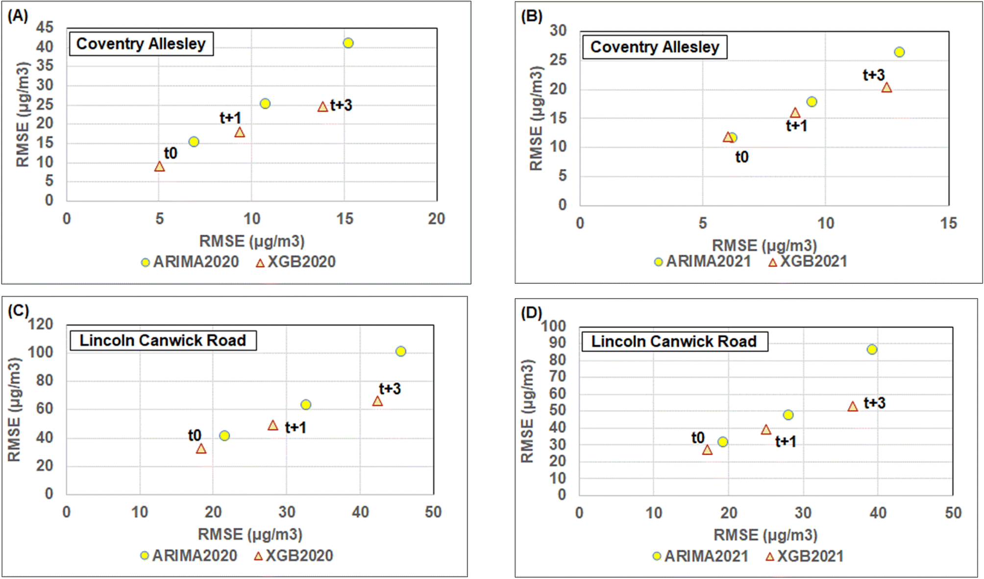Fig. 10 ARIMA and XGB NOx air quality prediction errors compared for time periods t0, t + 1 and t + 3 for the Coventry Allesley site: (A) 2020; and, (B) 2021; and the Lincoln Canwick Road site: (C) 2020; and, (D) 2021. The XGB trend-attribute models outperform ARIMA models for the urban background and roadside sites evaluated.

5. Discussion

The results presented demonstrate that accurate hourly predictions of NOx based on univariate recorded hourly trends at various city sites within the same geographic region are quite difficult to generate with MLR and ML models for periods much more than four hours ahead of the latest recorded data (t + 3). Not only does the magnitude of the NOx air concentrations vary quite rapidly from hour to hour with multiple short-lived spikes at each site, but it also varies substantially between the city sites studied. Fig. 11 illustrates the typical NOx recorded trends of an urban background (e.g., Coventry) and an urban roadside site (Lincoln) expressed on a 15 days moving average.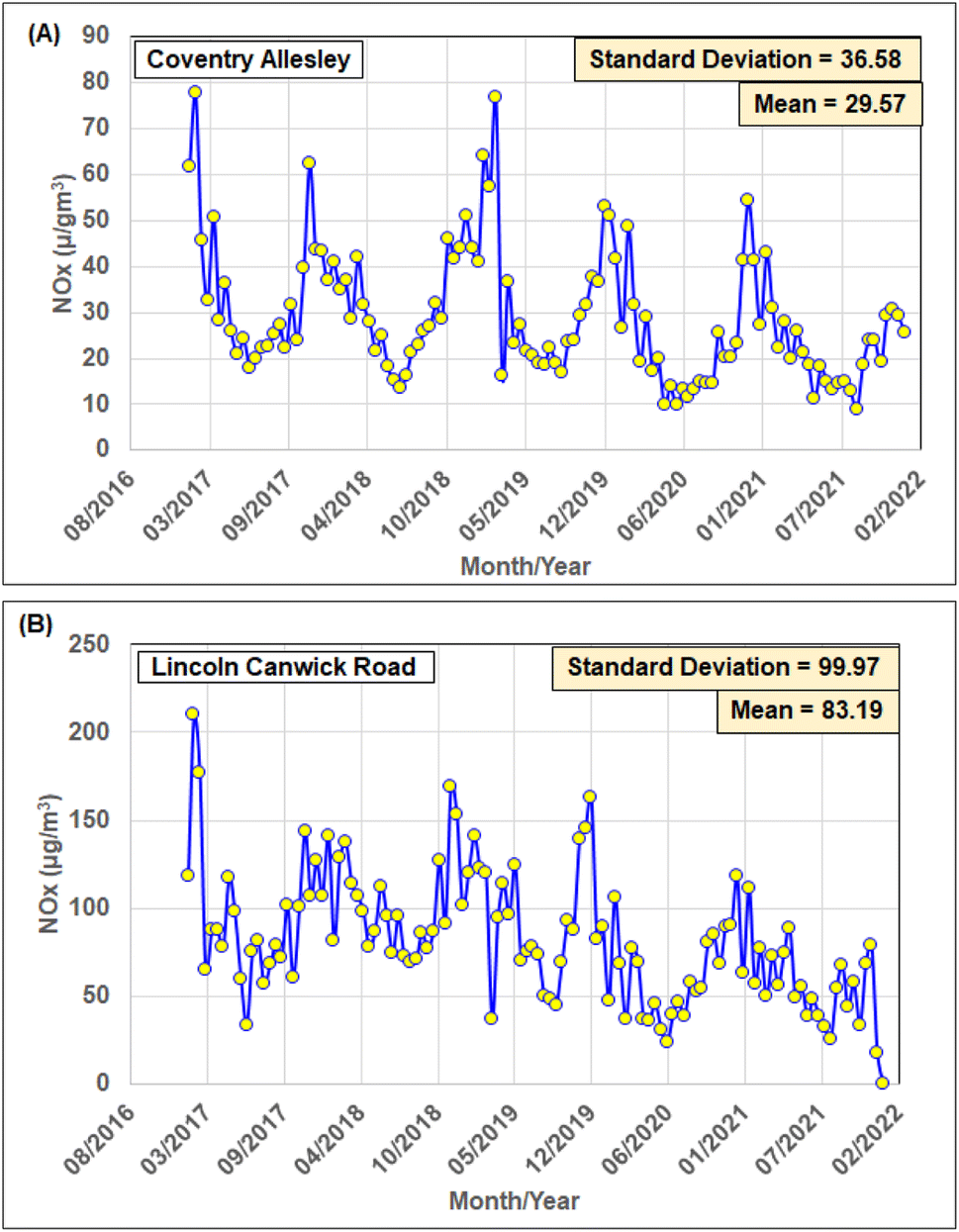

Fig. 11 15 days moving averages of recorded NOx hourly air quality values compared for: (A) Coventry Allesley (urban background recording site); and (B) Lincoln Canwick Road (urban roadside recording site). Both the urban background and roadside sites studied display distinctive annual and seasonal trends for the 2017 to 2021 period.

Undoubtedly, short-term weather conditions, including wind speed, relative humidity, air pressure, and precipitation, have some impacts on the hour-by-hour fluctuations in NOx levels at specific sites. For two of the years studied (e.g., 2020 and 2021) the magnitude of NOx air concentrations is lower with smaller peaks than in other years. Both sites displayed in Fig. 11 show broad declining trends from 2017 to 2021. However, the NOx air quality concentrations were substantially influenced by the reduced urban traffic flow and reduced industrial activity associated with COVID-19-driven lockdowns in 2020. Reduced traffic flows also persisted in 2021 due in part to more individuals working from home and continued reduced industrial activity in 2021. Hence, it is unwise to assume that under improved economic conditions NOx air concentrations in the studied cities will sustain the low levels recorded in 2020 and 2021 or that downward trends in NOx concentrations will persist in future years.

Fig. 11 also highlights that the spikiness of the NOx hourly data is much greater at the three roadside recording sites than at the urban background sites. This is to be expected as varying traffic volumes at contrasting times of the day and during weekdays versus weekends have a greater influence on NOx concentrations at the roadside recording site. A more detailed analysis of the magnitude of the spikiness in the recorded NOx data at the eight city sites reveals that this characteristic plays a relatively significant role in determining how easily and accurately short-term hourly forecasts of NOx air concentrations can be generated. Table 10 presents the mean absolute magnitude of hourly change (spike_mean), which is equivalent to the naïve forecast MAE value (Table 8), and the maximum absolute magnitude of hourly change (spike_max) in NOx concentrations recorded for different intervals in the 2017 to 2021 period, for each of the eight city sites studied.

Table 10 Magnitude of change in hourly recorded NOx air quality values at eight city sites from Central England during different periods from 2017 to 2021. The mean hourly change in NOx is greater at the roadside site than the urban background sites for all time intervals considered

Absolute hourly change in recorded NOx air quality
Recording stations	2017–2019		2020		2021
	Mean (μg m^−3)	Maximum (μg m^−3)	Mean (μg m^−3)	Maximum (μg m^−3)	Mean (μg m^−3)	Maximum (μg m^−3)
Coventry Allesley	9.06	311.72	6.34	270.80	5.83	222.38
Leeds Centre	11.27	434.80	6.98	159.40	7.71	228.65
Leicester University	9.43	445.65	7.19	260.12	7.21	185.48
Lincoln Canwick Road	31.21	613.16	20.39	551.80	18.38	255.55
Nottingham Centre	10.53	441.83	6.41	340.57	7.09	231.00
Sheffield Barnsley Road	26.09	733.37	19.85	496.13	22.40	399.73
Sheffield Devonshire Green	9.50	532.00	7.28	416.33	9.31	295.61
York Fishergate	16.94	440.93	10.35	405.39	10.10	226.81

---

It is apparent from Table 10 that the roadside recording sites are associated with substantially higher spike_mean and spike_max values than the urban background sites. Moreover, the urban recording sites associated with the smoothest data (lowest spike_mean values) are Coventry Allesley and Nottingham Centre. In particular, the period 2020 at the Nottingham and Coventry sites and 2021 at the Coventry site are associated with some of the smoothest data of all the sites and periods evaluated. It is considered to be of no coincidence that these periods for these specific sites are predicted with similar or slightly lower errors by the naïve forecasts than by the trend-attribute-based ML models. However, such relatively smooth NOx hourly trends are quite unusual, making the naïve forecasts unreliable for NOx t0 predictions over multiple years.

The results presented justify the use of trend-attribute-supported univariate NOx forecasts up to four hours ahead involving attributes calculated for the available hourly data from the previous hours t − 12 to t − 1. Future studies are required to see whether it is possible to improve the t0 to t + 3 NOx forecasts by (1) using additional or alternative trend attributes; (2) segregating the data into separate months to focus on specific seasonal influences; and (3) segregating the data into distinct weekday and weekend groups to distinguish the diverse types of anthropogenic activities influencing those specific days. Moreover, the timing and duration of short-lived NOx spikes are highly likely to be influenced to varying extents by prevailing weather conditions. Hence, future studies are also recommended to evaluate combining the trend-attribute method with various meteorological variables to see if the prediction of the NOx spike values, particularly for the t + 3 period, could be improved.

NOx hourly air concentration trends at most sites do experience diurnal fluctuations, caused by changes in traffic volumes and industrial activity. Whereas this study focuses on trend attributes extracted from data recorded over the past twelve hours, it is worth considering trend attributes from the past twenty-four hours or longer in attempts to capture more of the diurnal component in the NOx hourly recorded trends. It is possible that such longer-range attributes could provide improved NOx predictions for t + 3 to t + 12 hours ahead. However, further studies are required to confirm that possibility.

As the world strives to achieve net-zero emissions, possibly moving towards more hydrogen-based energy supply the monitoring of NOx air quality trends will become even more important than they are today. Contrary to the statements made by some corporations, combusting hydrogen in power plants is not emission-free. Although doing so avoids carbon dioxide emissions it has the potential to substantially increase NOx emissions.⁴⁰ Hydrogen is a small atom that leaks easily into the atmosphere causing the formation of water, methane, and ozone, which may also have impacts locally on NOx trends.¹¹ Hence, the ability to monitor NOx trends at city sites and reliably predict NOx air concentrations for the hours ahead at specific city sites is an important aspiration making trend-attribute prediction analysis a worthwhile approach to develop.

6. Summary of findings and conclusions

Trend attributes can be usefully extracted from oxides of nitrogen (NOx) air-concentration time series to predict using machine learning (ML) models hours-ahead NOx without recourse to exogenous data related to meteorology, traffic movements, or background air pollution data. Fifteen trend attributes, including seasonality components and simple differences between NOx levels in the past twelve hours (t − 12 to t − 1), are extracted from the hourly recorded NOx trends from 2017 to 2021 for eight city recording stations in Central England (five in background locations and three at roadside locations). These trend attributes capture subtleties in the NOx trends of the past few hours that regression ML models can exploit for prediction purposes. The city datasets capture reduced NOx emission trends in 2020 and 2021 related to reduced traffic-related and industrial activity due to the COVID-19 lockdown and associated economic recession.

The datasets are evaluated, on a supervised basis, with four NOx prediction models: multi-lateral regression, K-nearest neighbour (KNN), support vector regression (SVR), and extreme gradient boosting (XGB). The SVR and XGB models provide the most accurate NOx predictions as they are better able to cope with the non-parametric relationships between many of the trend attributes and NOx. These two models also typically outperform naïve forecasts, moving averages, and autoregressive prediction methods with the compiled city datasets. For t0 (one hour ahead of the latest recorded NOx data), the SVR and XGB models trained with 2017 to 2019 data to predict 2020 hourly NOx data or trained with 2017 to 2020 data to predict 2021, do so with mean absolute errors (MAE) ranging between 5 and 7 μg m⁻³ for urban background sites and between 9 and 20 μg m⁻³ for urban roadside recording sites. Similar errors are generated using models trained with 2021 data to predict 2020 hourly NOx, and vice versa. This indicates that the trend-attribute method can accommodate substantial fluctuations in NOx concentrations from one year to another and still provide NOx hourly predictions with consistent levels of accuracy.

For t + 1 (two hours and four hours ahead of the latest recorded NOx data, respectively), XGB models trained with 2017 to 2019 data to predict 2020 hourly NOx data or trained with 2017 to 2020 data to predict 2021, do so with mean absolute errors (MAE) ranging between 6 and 14 μg m⁻³ for urban background sites and between 14 and 29 μg m⁻³ for urban roadside recording sites. For t + 3 the same configuration of XGB, predictions generate mean absolute errors (MAE) ranging between 14 and 18 μg m⁻³ for urban background sites and between 20 and 42 μg m⁻³ for urban roadside recording sites. For t + 1 forecasts, the MAE range equates to between 2% and 4% of the recorded NOx value ranges for 2020 and 2021 at the eight city sites. Whereas, for t + 3 forecasts, the MAE range equates to between 2% and 7% of the recorded NOx value ranges for 2020 and 2021 at the eight city sites. Such error magnitudes indicate that the trend attribute model provides NOx hourly forecasts with reasonable accuracy at least four hours ahead of the available recorded data. However, the low correlation coefficients between predicted and measured NOx t + 3 values, due mainly to the peak values being underestimated by the prediction models, indicate that there is substantial room for improvement when predicting four hours ahead using this univariate method. Future studies are required to evaluate whether the combination of trend attributes with selected meteorological variables would improve the t + 3 peak NOx prediction accuracy.

The method evaluated offers a flexible, transparent, and reliable way to provide near-term, hour-ahead NOx forecasts at local sites avoiding the complication of using exogenous weather-related or environmental variables. However, it is considered likely that the combination of the trend attribute with certain meteorological variables would improve the prediction accuracy of the NOx peaks, particularly for t + 3 forecasts.

Analysis of the spikiness of the NOx hourly trends at the eight city sites reveals that those recorded at the urban background sites are noticeably smoother (much fewer peaks of whatever magnitude) than the urban roadside sites. This is consistent with greater influences from traffic emissions at the roadside sites and explains why NOx trends at the roadside sites generate higher prediction errors than urban background sites.

Feature importance analysis provided by the XGB models indicates the t − 1 attribute is the single most important attribute in the NOx t0 predictions at both background and roadside sites. For t + 1 predictions the t − 1 attribute still dominates but the ANOx(−1 to −3) also has a substantial influence at the background sites, whereas the DNOx(−12 to −1), RNOx(−3 to −1), and DNOx(−3 to −1) attributes exert substantial influence at the roadside sites. For t + 3 predictions, the t − 1 attribute becomes the second most influential attribute with ANOx(−1 to −12) dominating at the background sites, whereas the DNOx(−12 to −1) dominates at the roadside sites. These results suggest that the XGB NOx hourly prediction models make more use of the attributes involving information from t − 12 to t − 3 as the prediction target moves forward from t0 to t + 3. In most cases, the variable influences of the trend attributes on hourly NOx predictions are consistent with their Pearson and Spearman correlation coefficients with recorded NOx.

The findings of this study confirm the ability of trend attributes calculated from recorded t − 12 to t − 1 NOx data to assist in the prediction of NOx up to four hours ahead (t0 to t + 3) of the recorded data. This provides sufficient encouragement for future studies to evaluate the prediction contributions of trend attributes extending back beyond t − 24 to capture more of the diurnal variations in hourly NOx data. Moreover, dividing the datasets into monthly subgroups and weekday versus weekend subgroups is also worthy of further evaluation with the trend-attribute method as this may also improve hourly NOx prediction accuracy.

Author contributions

David Wood is sole author and is responsible for all aspects of data compilation, analysis, interpretation and writing.

Conflicts of interest

The author declares that he has no conflicts of interest.

Appendix A

The five graphs (A) to (E) displayed here are included to complement the multi-year trends shown in Fig. 1 by displaying that data on an annual basis. The data displayed represents 15 days rolling averages of hourly NOx air quality data recorded at eight city sites in Central England for years 2017, 2018, 2019, 2020, and 2021. These are raw data trends including periods where no data was recorded (data gaps).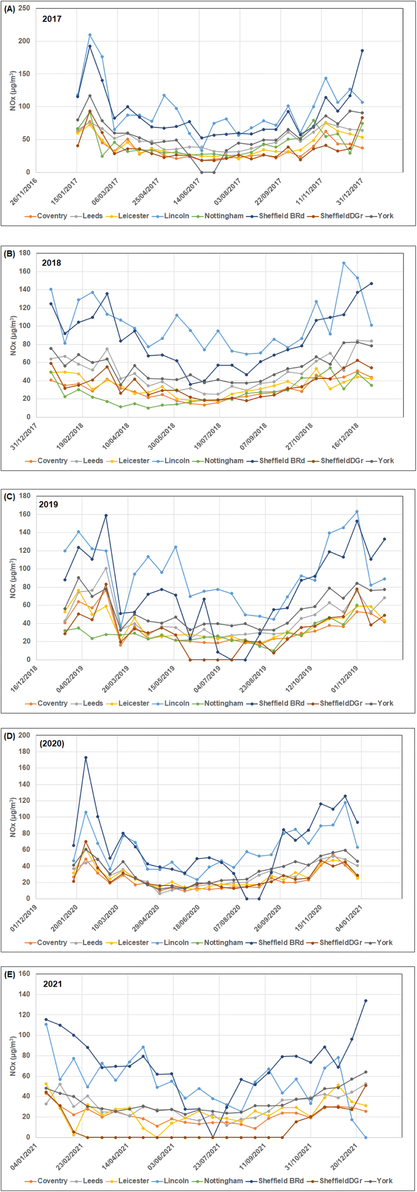

References

1. D. Fowler, P. Brimblecombe, J. Burrows, M. R. Heal, P. Grennfelt and D. S. Stevenson, et al., A chronology of global air quality, Philos. Trans. R. Soc., A, 2020, 378, 20190314,  DOI:10.1098/rsta.2019.0314.
2. N. Künzli, R. Kaiser, S. Medina, M. Studnicka and O. Chanel, et al., Public-health impact of outdoor and traffic-related air pollution: a European assessment, Lancet, 2000, 356(9232), 795–801,  DOI:10.1016/S0140-6736(00)02653-2.
3. A. J. Cohen, M. Brauer, R. Burnett, H. R. Anderson, J. Frostad and K. Estep, et al., Estimates and 25-year trends of the global burden of disease attributable to ambient air pollution: an analysis of data from the Global Burden of Diseases Study 2015, Lancet, 2017, 389(10082), 1907–1918,  DOI:10.1016/S0140-6736(17)30505-6.
4. F. Caiazzo, A. Ashok, I. A. Waitz, S. H. L. Yim and S. R. H. Barrett, Air pollution and early deaths in the United States. Part I: Quantifying the impact of major sectors in 2005, Atmos. Environ., 2013, 79, 198–208,  DOI:10.1016/j.atmosenv.2013.05.081.
5. L. Pimpin, L. Retat, D. Fecht, L. de Preux, F. Sassi and J. Gulliver, et al., Estimating the costs of air pollution to the National Health Service and social care: An assessment and forecast up to 2035, PLoS Med., 2018, 15(7), e1002602,  DOI:10.1371/journal.pmed.1002602.
6. EPA, Ecosystems and Air Quality, Environmental Protection Agency, 2021, https://www.epa.gov/eco-research/ecosystems-and-air-quality, accessed 12th January 2023.
7. R. M. Hoesly and S. J. Smith, et al., Historical (1750–2014) anthropogenic emissions of reactive gases and aerosols from the Community Emissions Data System (CEDS), Geosci. Model Dev., 2018, 11, 369–408,  DOI:10.5194/gmd-11-369-2018.
8. C.-P. Kuo and J. S. Fu, Ozone response modeling to NOx and VOC emissions: Examining machine learning models, Environ. Int., 2023, 176, 107969,  DOI:10.1016/j.envint.2023.107969.
9. W. R. Stockwell, C. V. Lawson, E. Saunders and W. S. Goliff, A review of tropospheric atmospheric chemistry and gas-phase chemical mechanisms for air quality modeling, Atmosphere, 2012, 3, 1–32,  DOI:10.3390/atmos3010001.
10. UK Government Statistics, Air quality statistics in the UK, 1987 to 2021 – nitrogen dioxide (NO₂), 28^th April 2022. https://www.gov.uk/government/statistics/air-quality-statistics/ntrogen-dioxide, accessed 12th January, 2023.
11. I. B. Ocko and S. P. Hamburg, Climate consequences of hydrogen emissions, Atmos. Chem. Phys., 2022, 22, 9349–9368,  DOI:10.5194/acp-22-9349-2022.
12. K. Szymankiewicz, J. W. Kaminski and J. Struzewska, Application of satellite observations and air quality modelling to validation of NOx anthropogenic EMEP emissions inventory over Central Europe, Atmosphere, 2021, 12, 1465,  DOI:10.3390/atmos12111465.
13. E. Giakoumis and A. Alafouzos, Study of diesel engine performance and emissions during a Transient Cycle applying an engine mapping-based methodology, Appl. Energy, 2010, 87, 1358–1365.
14. B. Degraeuwe, P. Thunis, A. Clappier, M. Weiss, W. Lefebvre, S. Janssen and S. Vranckx, Impact of passenger car NOX emissions on urban NO₂ pollution – scenario analysis for 8 European cities, Atmos. Environ., 2017, 171, 330–337,  DOI:10.1016/j.atmosenv.2017.10.040.
15. R. K. Maurya and P. Mishra, Parametric investigation on combustion and emissions characteristics of a dual fuel (natural gas port injection and diesel pilot injection) engine using 0-D SRM and 3D CFD approach, Fuel, 2017, 210, 900–913.
16. S. A. Provataris, N. S. Savva, T. D. Chountalas and T. Hountalas, Prediction of NOx emissions for high speed DI diesel engines using a semi-empirical, two-zone model, Energy Convers. Manage., 2017, 153, 659–670.
17. J. P. Shi and R. M. Harrison, Regression modelling of hourly NOx and NO₂ concentrations in urban air in London, Atmos. Environ., 1997, 31(24), 4081–4094,  DOI:10.1016/S1352-2310(97)00282-3.
18. K. Zhang, J. Thé, G. Xie and H. Yu, Multi-step ahead forecasting of regional air quality using spatial-temporal deep neural networks: A case study of Huaihai Economic Zone, J. Cleaner Prod., 2020, 277, 123231,  DOI:10.1016/j.jclepro.2020.123231.
19. Z. Li, S. H. Yim and K. F. Ho, High temporal resolution prediction of street-level PM2.5 and NOx concentrations using machine learning approach, J. Cleaner Prod., 2020, 268, 121975,  DOI:10.1016/j.jclepro.2020.121975.
20. J. A. Kamińska, A random forest partition model for predicting NO₂ concentrations from traffic flow and meteorological conditions, Sci. Total Environ., 2019, 651(1), 475–483,  DOI:10.1016/j.scitotenv.2018.09.196.
21. D. A. Olson, T. P. Riedel, J. H. Offenberg, M. Lewandowski, R. Long and T. E. Kleindienst, Quantifying wintertime O3 and NOx formation with relevance vector machines, Atmos. Environ., 2021, 259, 118538,  DOI:10.1016/j.atmosenv.2021.118538.
22. G. E. Kulkarni, A. A. Muley, N. K. Deshmukh and P. U. Bhalchandra, Autoregressive integrated moving average time series model for forecasting air pollution in Nanded city, Maharashtra, India, Model. Earth Syst. Environ., 2018, 4, 1435–1444,  DOI:10.1007/s40808-018-0493-2.
23. E. Marinov, D. Petrova-Antonova and S. Malinov, Time series forecasting of air quality: a case study of Sofia City, Atmosphere, 2022, 13, 788,  DOI:10.3390/atmos13050788.
24. Z. Zhao and Y. Ma, Research on multi-step prediction of inlet NOx concentration based on VMD-ARIMA model, 2021 40th Chinese Control Conference (CCC), Shanghai, China, 2021, pp. 1303–1308,  DOI:10.23919/CCC52363.2021.9550026.
25. A. Al Yammahi and Z. Aung, Forecasting the concentration of NO₂ using statistical and machine learning methods: A case study in the UAE, Heliyon, 2023, 9(2), e12584,  DOI:10.1016/j.heliyon.2022.e12584.
26. B. Liu, L. Zhang, Q. Wang and J. Chen, A novel method for regional NO₂ concentration prediction using discrete wavelet transform and an LSTM network, Comput. Intell. Neurosci., 2021, 6631614, 14,  DOI:10.1155/2021/6631614.
27. D. A. Wood, Near ground-level ozone air concentration trend attributes assist hours-ahead forecasts avoiding exogenous data inputs, Urban Clim., 2023, 47, 101382,  DOI:10.1016/j.uclim.2022.101382.
28. UK Air, Air information resource, 2023, https://uk-air.defra.gov.uk/, accessed 12th January 2023.
29. Statsmodels, Statistical models in Python: seasonal decompose, 2023, https://www.statsmodels.org/stable/generated/statsmodels.tsa.seasonal.seasonal_decompose.html, accessed 12th January 2023.
30. SciKit Learn, Supervised and unsupervised machine learning models in Python, 2023, https://scikit-learn.org/stable/, accessed 12th January 2023.
31. F. E. Harrell, Regression Modeling Strategies, Springer, Switzerland, 2nd edn, 2015, p. 582,  DOI:10.1007/978-3-319-19425-7.
32. E. Fix, and J. L. Hodges, Discriminatory analysis, nonparametric discrimination: consistency properties, Technical Report, USAF School of Aviation Medicine, 1951.
33. C. Cortes and V. Vapnik, Support-Vector Networks, Mach. Learn., 1995, 20(3), 273–297,  DOI:10.1007/BF00994018.
34. Y. W. Chang, C. J. Hsieh, K. W. Chang, M. Ringgaard and C. J. Lin, Training and testing low-degree polynomial data mappings via linear SVM, J. Mach. Learn. Res., 2010, 11(4), 1471–1490,  DOI:10.5555/1756006.1859899.
35. T. Chen and C. Guestrin, XGBoost: a scalable tree boosting system, in Proceedings of the 22nd ACM SIGKDD International Conference on Knowledge Discovery and Data Mining, ed. Krishnapuram, B., Shah, M., Smola, A. J., Aggarwal, C. C., Shen, D. and Rastogi, R., San Francisco, CA, USA, August 13–17, 2016, ACM: 785–794,  DOI:10.1145/2939672.2939785.
36. GridSearchCV, Grid search of hyperparameters by SciKit over a range of estimator hyperparameters, SciKit Learn, 2023, https://scikit-learn.org/stable/modules/generated/sklearn.model_selection.GridSearchCV.html, accessed 12th January 2023.
37. BayesSearchCV, Bayesian optimization of hyperparameters by SciKit optimization, 2023, https://scikit-optimize.github.io/stable/modules/generated/skopt.BayesSearchCV.html, accessed 12th January 2023.
38. D. A. Wood, Machine learning and regression analysis reveal different patterns of influence on net ecosystem exchange at two conifer woodland sites, Res. Ecol., 2022, 4(2), 24–50,  DOI:10.30564/re.v4i2.4552.
39. R. Boddy and G. Smith, Statistical Methods in Practice: For scientists and technologists, Chichester UK Wiley, 2009, pp. 95–96, ISBN 978-0-470-74664-6.
40. M. S. Cellek and A. Pınarbaşı, Investigations on performance and emission characteristics of an industrial low swirl burner while burning natural gas, methane, hydrogen-enriched natural gas and hydrogen as fuels, Int. J. Hydrogen Energy, 2018, 43(2), 1194–1207,  DOI:10.1016/j.ijhydene.2017.05.107.

---