 Open Access Article
Machine learning classification of polar sub-phases in liquid crystal MHPOBC
Rebecca
Betts
and
Ingo
Dierking
 *
*
Department of Physics and Astronomy, University of Manchester, Oxford Road, Manchester M139PL, UK. E-mail: ingo.dierking@manchester.ac.uk
First published on 23rd August 2023
Abstract
Experimental polarising microscopy texture images of the fluid smectic phases and sub-phases of the classic liquid crystal MHPOBC were classified as paraelectric (SmA*), ferroelectric (SmC*), ferrielectric (SmC1/3*), and antiferroelectric (SmCA*) using convolutional neural networks, CNNs. Two neural network architectures were tested, a sequential convolutional neural network with varying numbers of layers and a simplified inception model with varying number of inception blocks. Both models are successful in binary classifications between different phases as well as classification between all four phases. Optimised architectures for the multi-phase classification achieved accuracies of (84 ± 2)% and (93 ± 1)% for sequential convolutional and inception networks, respectively. The results of this study contribute to the understanding of how CNNs may be used in classifying liquid crystal phases. Especially the inception model is of sufficient accuracy to allow automated characterization of liquid crystal phase sequences and thus opens a path towards an additional method to determine the phases of novel liquid crystals for applications in electro-optics, photonics or sensors. The outlined procedure of supervised machine learning can be applied to practically all liquid crystal phases and materials, provided the infrastructure of training data and computational power is provided.
1 Introduction
Artificial Intelligence (AI) and Machine learning (ML) algorithms have existed since the 1950s1 but have only recently seen significant improvements allowing them to be fully utilised. This is particularly due to increased computing power, but also developments in the algorithms themselves such as the introduction of non-linearity and the back-propagation algorithm. There has also been an increase in the availability of the large datasets required for ML.2 Convolutional neural networks are a type of ML algorithm which use a convolution operation to extract features from input images or other grid-based data [ref. 3 and references therein]. They have shown particular success in medical imaging applications4–6 especially in cancer research7,8 for example in mitosis detection in breast cancer histology images.9 The use of machine learning can currently be followed through all fields of sciences, for example biology through the use in biosensors,10 in chemistry for drug discovery11 and in the computer-aided synthesis planning,12 in material science13 and physics14 for example in nano-photonics,15 but also astronomy16–18 and particle physics.19Besides this admittedly inconclusive list of examples, machine learning is of course also employed in the study of condensed matter phases and phase transitions,20 which links to the investigations of liquid crystals and soft matter.21–23 The success of machine learning techniques in the characterization of liquid crystals has so far been demonstrated in various aspects of LC research. The prediction of phase transitions has been one of the major issues,24–27 with work concentrating on the isotropic to nematic transition of thermotropic liquid crystals being studied with simulated Schlieren-textures but also with experimental images. Other investigations were concerned with theoretical predictions of the molecular ordering of binary mixtures of molecules with different length,28 the self-assembled nanostructures of lyotropic liquid crystals29 and the local structure of liquid crystalline polymers.30 Another issue, which is still in its infancy is the prediction of physical properties by machine learning, as demonstrated recently by a comparison of the experimental and predicted dielectric properties of a nematic liquid crystal.31
Much of the machine learning work on liquid crystals so far is related to object detection32 and specifically directed towards topological defects in nematics, i.e. the above mentioned Schlieren-textures. For such investigations simulated33 as well as experimental34 textures have been employed. A particularly interesting example was that of an active nematic which was studied in relation to hydrodynamics.35 Proposing a similar background, an investigation has been reported where machine learning is employed to detect islands and bubbles in smectic films,36 providing an accuracy which exceeds conventional tracking software.
Considering the applicational side of machine learning being used in relation to liquid crystals, one needs to mention a variety of sensors,37 which are all based on stimulated texture transitions of nematic LCs. The general idea was introduced by the Abbott group38 and later applied to biochemical sensors,39 for example in the detection of endotoxins from different bacterial species,40 but also during the recent pandemic for the detection of SARS-CoV-2.41 With a rather similar experiment the general sensor ideas can also be employed to detect gases42 and gas mixtures.43
In recent times we have tested methodologies to apply machine learning algorithms not only for the simple transition from the isotropic to nematic phase, or texture transitions from homeotropic to planar, but rather for the identification of whole liquid crystal phase sequences.44 These were based on convolutional neural networks as well as inception models with varying numbers of layers, inception blocks, and regularization methods. They were applied to a range of different phases including isotropic, nematic, cholesteric, smectic A, smectic C, and the hexatic phases smectic I and smectic F.45 While binary classifiers resulted in prediction accuracies of larger than 97%, even the prediction of the whole phase sequence, had an accuracy of about 90%, which is certainly satisfactory for a first prediction attempt with a limited number of images and computing facilities. Also phase transitions and transition temperatures could in most cases be very well predicted46 with accuracies well above 90% and relative temperature accuracies limited by the experimental resolution of the employed hot stage (±0.1 K).
In this study we extend similar phase identification methodologies to chiral liquid crystals and their polar phases. In particular, we have investigated the classic material 4-(1-methylheptyloxycarbonyl)phenyl 4′-octyloxybiphenyl-4-carboxylate, (MHPOBC). This exhibits on cooling the paraelectric smectic A* phase, smectic Cα*, ferroelectric smectic C*, ferrielectric smectic C1/3* and antiferroelectric smectic CA*. It will be demonstrated that in addition to different classes of phases (fluid, hexatic, soft crystal) machine learning is also able to distinguish between more subtle phases, when appropriately trained.
2 Experimental
2.1 Liquid crystal material and phases
The discovery of ferroelectricity in liquid crystals goes back to the symmetry arguments of Meyer et al. and was first demonstrated in a pioneering publication47 in 1975. In essence it was argued that every chiral, tilted smectic phase can in principle exhibit a spontaneous polarization PS and would therefore be pyroelectric. If this spontaneous polarization can be switched between two stable states by an applied electric field, the material is termed to be ferroelectric. This would for example be the case for the fluid smectic C* (SmC*) phase and the hexatic smectic I* (SmI*) and smectic F* (SmF*) phases. The asterix (*) here denotes molecular chirality. Yet, in order to compensate the spontaneous polarization over short distances, the ferroelectric phases adopt a helical superstructure, due to the coupling between polarization and tilt angle, which in optical polarization microscopy (POM) is often visible as an equidistant line pattern. More correctly, the SmC* phase should therefore be called helielectric, because the polarization is compensated. Nevertheless, when subjecting the phase to boundary conditions such that the cell gap is much smaller than the helical pitch, the helix is unwound and a domain texture with two stable states is observed. This is called the surface stabilized ferroelectric liquid crystal (SSFLC) geometry, invented by Clark and Lagerwall,48 which is of outmost importance for applications of ferroelectric liquid crystals (FLC). In the investigations presented here, we will rely on bulk samples, which in POM show a fan-like texture (SmA*) or broken fan-like texture (SmC*) with focal conics.49 Several years later, antiferroelectricity was demonstrated for the compound MHPOBC,50–52 which is a chiral, calamitic mesogen with the following structural formula:Later, other subphases were discovered, such as the SmCα* phase, located between SmA* and SmC*,52 which exhibits an (incommensurate) helical superstructure with very small pitch, well below the resolution limit of POM,53 which explains why this phase can hardly be distinguished from SmA* by microscopy alone. And indeed, also machine learning algorithms are therefore not capable to distinguish both phases, because there are no structurally distinguishing features observed by microscopy. This is the reason why we will only shortly mention the SmCα* phase below in the results section and otherwise omit it from further investigation.
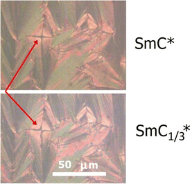
At last, the so-called ferrielectric phase54,55 SmC1/3* is found between the ferroelectric SmC* and the antiferroelectric SmCA* phase. (In fact, this phase should also be called helielectric, because it does not exhibit a polarization at zero applied electric field.) There is one striking structural feature that distinguishes the ferrielectric phase from both its ferroelectric as well as its antiferroelectric counterparts. In the ferrielectric phase the focal conic defects split up56 as shown in Fig. 1.
At lower temperatures when the ferrielectric to antiferroelectric phase transition is crossed, the defects will merge again. It physical reason for this phenomena does not seem to be unveiled, but is observed for different compounds as well and can thus be recognized by machine learning as a distinguishing structural feature. The phase sequence of the fluid phases as determined by polarizing microscopy on cooling is thus: Iso 149 SmA* 122 SmCα* 121 SmC* 119 SmC1/3* 118 SmCA* and is shown in Fig. 2.
Experimental image acquisition was carried out with a Leica DMLP polarizing microscope in combination with a Linkam TP94 temperature controller and LTSE350 hot stage, equipped with a digital camera (IDS uEye at resolution of 2048 × 1088 pixels). Already visually from Fig. 2 it becomes clear that the classification of the different phases of MHPOBC will not be a trivial task by machine learning algorithms, because the structural features distinguishing between the different phases are minimal, especially as changes in birefringence, i.e. slight color changes in the texture photographs cannot be chosen as a criteria.
2.2 Machine learning for classification
This project aims to develop a machine learning algorithm to classify LC phases using polarising microscopy images of their textures. The algorithm is some function mapping the pixel values of the input image, a matrix X, to a vector of the probabilities of the image belonging to each possible images from the phase, which can be taken as the predicted phase label, ŷ,| ŷ = f(X,θ) | (1) |
 | (2) |
| f[l](zi) = max(0,zi) | (3) |
 | (4) |
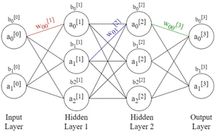 | ||
| Fig. 3 Schematic of neural network with two hidden layers and weights, biases, and activations labelled. | ||
As discussed above, the training examples are passed through the network and the parameters of the function in eqn (1), the weights and biases, are updated. Often, however, the training data is split into equally sized batches, and the parameters are updated after each batch is passed through the network, speeding up training. The loss function is taken as the average of the loss functions of each training example in the batch. Batches are used primarily to reduce the amount of memory required to load the data. Because the loss function is dependent on all parameters in the network, its derivative with respect to each parameter can be calculated, starting with the final layer, then applying the derivative chain rule for each preceding layer, working backwards in a process known as backpropagation. This gives the gradient of the loss function in the dimensional space of all parameters. By choosing a learning rate, α, each weight and bias can be updated as
 | (5) |
The loss function gives a measure of the difference between the true and predicted labels and can be defined in many ways. For classification tasks, categorical cross-entropy, LCE, is generally used. This is defined for a training example with true label, yn, and predicted label, ŷn, as
 | (6) |
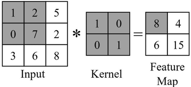
One advantage of convolutional neural networks is that they make use of the same trainable parameters over the whole area of the image, reducing computational cost in comparison to the standard neural networks discussed previously.60
Data augmentation involves artificially increasing the dataset size by creating modified copies of the training set images. Based on previous studies,28,45 each image in the training dataset was reflected horizontally and vertically, tripling the dataset size.
Dropout regularisation involves randomly setting the output of nodes to zero with a given probability (the dropout rate). It is applied to dense layers only and prevents the network relying on any particular feature by forcing new pathways to be created. As a result, the network takes more epochs to train.61
When a network overfits, particular weights will grow to be very large. L2 regularisation discourages this by adding a term to the loss function (eqn (7)),
 | (7) |
Batch normalisation involves rescaling the outputs to a layer using two trainable parameters, γ and β, such that that output, z, is normalised as
 | (8) |
3 Methodology
3.1 Configuring models
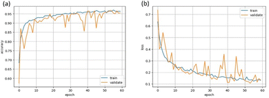
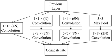
Two different architectures of CNNs where compared according to their performance in the task of classifying LC phases, the sequential and inception models detailed below. Both models used the Adam optimisation algorithm,65 categorical cross-entropy as the loss function and ReLU activation in all layers except for the output (which uses softmax activation). All convolutional layers had a stride of 1 × 1 and were followed by batch normalisation. Dropout was applied to all dense layers, and L2 regularisation to both dense and convolutional layers. All models were trained with a batch size of 64. The binary classifiers used a learning rate of 5 × 10⁻⁵ and the multiphase classifiers used a learning rate of 1 × 10⁻⁴.The hyperparameters, parameters that control the learning process such as learning rate and number of convolutional layers, were optimised for each model, based on the criteria of achieving the greatest validation accuracy. Each model was monitored during training by plotting both the training and validation datasets’ accuracy and loss at each epoch, providing the learning curve. Successful training could be recognised by similar training and validation curves, reaching a plateau at the maximum accuracy and minimum loss. An illustrative example for the accuracy and loss learning curves is depicted in Fig. 5. All possible combinations of hyperparameters could not be tested, so optimisation was achieved by beginning with a small model (for example one convolutional and one dense layer) and then increasing the model size incrementally until overfitting was seen. Other hyperparameters such as batch size, learning rate and dropout rate were also varied until suitable learning curves were seen. All models showed some spikes in the validation loss and corresponding dips in the validation accuracy throughout training, possibly due to the limited dataset size meaning there was some dissimilarity between the validation and training datasets. These spikes were reduced by decreasing the learning rate, however could not be minimised entirely as this also significantly increased the training time. To prevent an epoch with very low validation accuracy being used to evaluate the test dataset, the epoch with highest validation accuracy was saved and tested. This was repeated three times, i.e. through three training cycles with the same hyperparamters, and the mean and standard deviation of the test dataset accuracy was calculated. There is some further uncertainty on the test accuracy due to the finite size of the test dataset, however this was found to be negligible. Therefore, the uncertainty on each accuracy is given just by the standard deviation of the three test accuracies. Both models were trained using GPUs provided by Google Colaboratory66 and implemented with Keras67 and TensorFlow libraries.68
3.2 Data preparation
Samples of MHPOBC were prepared between glass slides without treatment for boundary conditions, such that they had a thickness of approximately 6 μm. Videos across phase transitions were recorded and images extracted via the VLC media player,70 with their true phase labels being assigned based on the POM characterisation. Each 2048 × 1088 pixel image was split into six 540 × 540 pixel squares. These were each converted to greyscale, scaled to a resolution of 256 × 256 and reflected horizontally and vertically to augment the dataset as discussed in Section 2.2.3.To prevent too much similarity between the training, validation and testing sets, the videos (rather than the images) were split between the sets at an approximate ratio of 70![[thin space (1/6-em)]](https://www.rsc.org/images/entities/char_2009.gif) :
:![[thin space (1/6-em)]](https://www.rsc.org/images/entities/char_2009.gif) 15
15![[thin space (1/6-em)]](https://www.rsc.org/images/entities/char_2009.gif) :
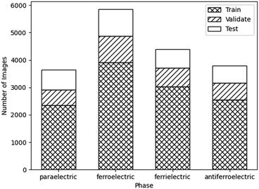
:![[thin space (1/6-em)]](https://www.rsc.org/images/entities/char_2009.gif) 15, respectively. If similar images taken from the same video would have been split between the three sets, the accuracy of the network on unseen data would be overestimated. By comparing the final accuracies of each dataset, the effect of bias in the input data could be monitored. Significant bias would lead to the network being unable to perform on unseen data, resulting in a low test accuracy. This is particularly important as the data augmentation applied propagates any bias in the original data. The number of images belonging to each phase is shown in Fig. 8.
15, respectively. If similar images taken from the same video would have been split between the three sets, the accuracy of the network on unseen data would be overestimated. By comparing the final accuracies of each dataset, the effect of bias in the input data could be monitored. Significant bias would lead to the network being unable to perform on unseen data, resulting in a low test accuracy. This is particularly important as the data augmentation applied propagates any bias in the original data. The number of images belonging to each phase is shown in Fig. 8.
At this point it is also reasonable to make a general comment about the determination of liquid crystal phases via neural networks. Given the fact that this is implemented by supervised machine learning, phase identification does of course depend on the ability of experts to correctly identify the phases of the training data. The identification of previously unseen data is therefore not resistant against expert errors in the selection of the training data. Yet, this is equivalent for any polarising microscopic study. For a large-scale implementation of machine learning to characterise liquid crystalline phase sequences of novel compounds, it will thus be necessary to collect large quantities of data images of different materials, which will be independently identified by several different experts. In this work we merely demonstrate the feasibility of such an idea.
4 Results
Before discussing the actual results we would like to make two preliminary comments. The first one is concerning the isotropic to SmA* transition. Like any other transitions involving the formation of the liquid crystalline state, this is, with the exception of well oriented homeotropic alignment which has been discussed in ref. 46, a simple classification task between black and bright. All models discussed in literature so far have had a classification accuracy very close to 100% for this case, so we will not discuss this in any further detail.The second issue is that of the SmCα* phase. The transition from SmA* to this phase did not exhibit any changes of structural features which could be observable in polarized microscopy. We suggest that this is due to the short pitch of the helical superstructure, which is far below the resolution limit of optical microscopy. As such, SmA* and SmCα* are optically equivalent, which implies that in the absence of any differences in structural appearance, machine learning algorithms can in principle not detect the latter phase from textures alone. After several unsuccessful attempts with different sample preparations we were thus forced to ignore the presence of the SmCα* phase, despite the fact that it has been demonstrated in literature, for example through polarization-analysed resonant X-ray scattering.71,72 If one would want to distinguish between SmA* and SmCα*, a completely different experimental methodology would need to be used, which allows a better resolution and therefore differentiation between the two phases. This would represent a very different study in itself and is thus outside the scope of this investigation.
4.1 Binary classifiers
| Paraelectric SmA* to ferroelectric SmC* | Sequential model | Inception model |
|---|---|---|
| Convolutional layers/inception modules | (8, 16, 32) | (1, 2) |
| Dense layers | (16, 8) | (8, 4) |
| Dropout rate | 0.5 | 0.5 |
| Trainable parameters | 6682 | 7036 |
| Validation accuracy | 0.912 ± 0.003 | 0.934 ± 0.008 |
| Test accuracy | 0.90 ± 0.01 | 0.92 ± 0.02 |
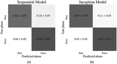
However, the inception model did require more parameters than for the previous binary classifier, using approximately 1.7 times the number of parameters to reach the same accuracy as the sequential model. Both models showed a slight bias towards the ferrielectric phase, despite the ferrielectric dataset being smaller. The optimised model architectures and their resulting accuracies are shown in Table 2, and the confusion matrices for each model are found in Fig. 10(a) and (b).
| Ferrielectric SmC1/3* to antiferroelectric SmCA* | Sequential model | Inception model |
|---|---|---|
| Convolutional layers/inception modules | (8, 16, 32) | (2, 2) |
| Dense layers | (16, 8) | (16, 8) |
| Dropout rate | 0.6 | 0.5 |
| Trainable parameters | 6682 | 11![[thin space (1/6-em)]](https://www.rsc.org/images/entities/char_2009.gif) 560 560 |
| Validation accuracy | 0.990 ± 0.003 | 0.996 ± 0.001 |
| Test accuracy | 0.986 ± 0.003 | 0.994 ± 0.002 |
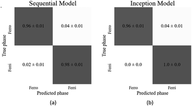
The sequential and inception models correctly classified the test images with accuracies of (98.6 ± 0.3)% and (99.4 ± 0.2)%, respectively, thus achieving very high accuracies for this transition. As the confusion matrices (Fig. 11(a) and (b)) show, there was no particular bias towards either dataset. In this task the inception model achieved a (0.8 ± 0.4)% higher accuracy than the sequential model. However, this small increase in accuracy required about 1.7 times as many parameters, so is at the expense of significantly increased computational cost. Table 3 displays the architecture details and resultant accuracies of each model.
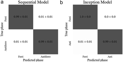 | ||
| Fig. 11 Confusion matrices of the best performing models for the ferrielectric (SmC1/3*) to antiferroelectric (SmCA*) transition for the (a) sequential and (b) inception model. | ||
| Ferroelectric SmC* to ferrielectric SmC1/3* | Sequential model | Inception model |
|---|---|---|
| Convolutional layers/inception modules | (8, 16, 32) | (2, 2) |
| Dense layers | (16, 8) | (16, 8) |
| Dropout rate | 0.6 | 0.5 |
| Trainable parameters | 6682 | 11![[thin space (1/6-em)]](https://www.rsc.org/images/entities/char_2009.gif) 560 560 |
| Validation accuracy | 0.97 ± 0.01 | 0.97 ± 0.01 |
| Test accuracy | 0.971 ± 0.004 | 0.977 ± 0.003 |
4.2 Multiphase classifier
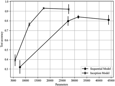
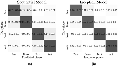
For the multiphase classification task, the inception model performed significantly better than the sequential model, resulting in test accuracies of (93 ± 1)% versus (84 ± 2)% respectively. The inception model also relied on comparatively fewer trainable parameters making it less computationally expensive. This demonstrates that the inception model is more suitable for this particular task and for more complex classification tasks in general, as highlighted in Fig. 12. The optimised model architectures and accuracies are shown in Table 4.| Multiphase | Sequential model | Inception model |
|---|---|---|
| Convolutional layers/inception modules | (8, 16, 32, 64) | (2, 2, 2) |
| Dense layers | (64, 32, 16, 8) | (16, 8) |
| Dropout rate | 0.6 | 0.4 |
| Trainable parameters | 31![[thin space (1/6-em)]](https://www.rsc.org/images/entities/char_2009.gif) 564 564 |
17![[thin space (1/6-em)]](https://www.rsc.org/images/entities/char_2009.gif) 420 420 |
| Validation accuracy | 0.84 ± 0.01 | 0.925 ± 0.002 |
| Test accuracy | 0.84 ± 0.02 | 0.93 ± 0.01 |
The confusion matrix for the sequential model (Fig. 13(a)) shows that the ferrielectric and antiferroelectric phases were only correctly classified in (84 ± 3)% and (87 ± 3)% of the cases, respectively. This is a significant decrease in comparison to the binary sequential classifier, which achieved (99 ± 1)% accuracy in classifying both of these phases. The multiphase inception model performed well in classifying these phases (see Fig. 13(b)), suggesting it may be better suited to handling multiphase classification.
5 Conclusions
It is demonstrated that supervised machine learning architectures like sequential convolutional neural networks CNNs and inception models can be employed to classify polar liquid crystals with phases such as the paraelectric SmA*, the ferroelectric SmC*, the ferrielectric SmC1/3* and the antiferroelectric SmCA* phase. This can be achieved via binary classifiers but also via multiphase classifiers with very good accuracies of the order of 90% and above. In the binary classification tasks, both the sequential and inception models achieved similar accuracies, suggesting no particular advantage of one over the other architecture. In the multiphase classification task, the inception model performed significantly better, achieving a test accuracy of (93 ± 1)% in comparison to (84 ± 2)% achieved with the sequential model. This suggests that a more complex classification problem is better approached with an inception than a sequential model.The investigation has further provided evidence that the characterisation of liquid crystals via texture observation can in the future be automated, provided that phases are studied which exhibit structural features that are different from those of other phases. Phases that appear identical cannot be identified individually from textures alone. Similarly, supervised machine learning as a texture characterization tool will also not be able to predict novel phases. Nevertheless, the presented results open a route to an additional characterization method, especially when sufficient training data is available, together with the needed computational infrastructure.
While the results show that CNNs are capable of classifying LC phases, a disadvantage of this method of classification is that it is difficult to extract information from the CNN on how the phases are distinguished. The CNN is a function approximating the relationship between input images and their labels, however this function involves thousands of parameters so cannot be used to give insight into any simple relationship between the input and the label. Analysis of the feature maps and kernels produced at each convolutional layer may give some information as to what features of an image the CNN uses, but there is a large number of these with complex interactions between them. As such, neural networks are often described as black box models, so the reasons behind the predictions they make cannot be understood. Although CNNs cannot directly be used to explain why a given phase displays a particular texture, by automating the task of classifying textures they can still contribute significantly to LC research. The ultimate vision of this and similar studies could be a sufficiently large database of all different liquid crystalline phases with varying boundary conditions, collected from a large range of different compounds and independently verified by a number of experts. This could then be used as training data, provided that sufficient computational power is available. With supervised machine learning algorithms of the CNN type with varying complexity, one could then automatically identify the large amounts of phase sequences of novel materials produced every year worldwide.
Author contributions
RB carried out the texture studies and the machine learning aspects of this study. ID conceived the investigation, supervised its implementation and contributed to the texture identification and writing of the manuscript.Conflicts of interest
There are no conflicts to declare.References
- H. D. Block, Rev. Mod. Phys., 1962, 34, 123–135 CrossRef.
- Y.-C. Wu and J.-W. Feng, Wireless Pers. Commun., 2018, 102, 1645–1656 CrossRef.
- A. Isozaki, J. Harmon, Y. Zhou, S. Li, Y. Nakagawa, M. Hayashi, H. Mikami, C. Lei and K. Goda, Lab Chip, 2020, 20, 3074–3090 RSC.
- A. Maier, C. Syben, T. Lasser and C. Riess, Z. Med. Phys., 2019, 29, 86–101 CrossRef PubMed.
- J.-G. Lee, S. Jun, Y.-W. Cho, H. Lee, G. B. Kim, J. B. Seo and N. Kim, Korean J. Radiol., 2017, 18, 570–584 CrossRef PubMed.
- M. Shehab, L. Abualigah, Q. Shambour, M. A. Abu-Hashem, M. K. Y. Shambour, A. I. Alsalibi and A. H. Gandomi, Comput. Biol. Med., 2022, 145, 105458 CrossRef PubMed.
- S. L. Goldenberg, G. Nir and S. E. Salcudean, Nat. Rev. Urol., 2019, 16, 391–403 CrossRef PubMed.
- A. Hosny, C. Parmar, J. Quackenbush, L. H. Schwartz and H. J. W. L. Aerts, Nat. Rev. Cancer, 2018, 18, 501–510 CrossRef PubMed.
- D. C. Cires, A. Giusti, L. M. Gambardella and J. Schmidhuber, Medical Image Computing and Computer-Assisted Intervention – MICCAI, 2013, Springer, Berlin, pp. 411–418 Search PubMed.
- F. Cui, Y. Yue, Y. Zhang, Z. Zhang and H. S. Zhou, ACS Sens., 2020, 5, 3346–3364 CrossRef CAS PubMed.
- H. Chen, O. Engkvist, Y. Wang, M. Olivecrona and T. Blaschke, Drug Discovery Today, 2018, 23, 1241–1250 CrossRef PubMed.
- C. W. Coley, W. H. Green and K. F. Jensen, Acc. Chem. Res., 2018, 51, 1281–1289 CrossRef CAS PubMed.
- L. Zhang and S. Shao, J. Appl. Phys., 2022, 132, 100701 CrossRef CAS.
- G. Carleo, I. Cirac, K. Cranmer, L. Laudet, M. Schuld, N. Tishby, L. Vogt-Maranto and L. Zdeborova, Rev. Mod. Phys., 2019, 91, 045002 CrossRef CAS.
- S. So, T. Badloe, J. Noh, J. Bravo-Abad and J. Rho, Nanophotonics, 2020, 9, 1041–1057 CrossRef.
- N. M. Ball and R. J. Brunner, Int. J. Mod. Phys. D, 2010, 19, 1049–1106 CrossRef.
- S. Sen, S. Agarwal, P. Chakraborty and K. P. Singh, Exp. Astron., 2022, 53, 1–43 CrossRef.
- S. K. Meher and G. Panda, Eur. Phys. J.-Spec. Top., 2021, 230, 2285–2317 CrossRef.
- A. Radovic, M. Williams, D. Rousseau3, M. Kagan, D. Bonacorsi5, A. Himmel, A. Aurisano, K. Terao and T. Wongjirad, Nature, 2018, 560, 41–48 CrossRef CAS PubMed.
- J. Carrasquilla and R. G. Melko, Nat. Phys., 2017, 13, 431–434 Search PubMed.
- P. S. Clegg, Soft Matter, 2021, 17, 3991–4005 RSC.
- A. L. Ferguson, J. Phys.: Condens. Matter, 2018, 30, 043002 CrossRef PubMed.
- T. Orlova, A. Piven, D. Darmoroz, T. Aliev, T. Mahmoud, T. Abdel Razik, A. Boitsev, N. Grafeeva and E. Skorb, Digital Discovery, 2023, 2, 298–315 RSC.
- H. Y. D. Sigaki, R. F. de Souza, R. T. de Souza, R. S. Zola and H. V. Ribeiro, Phys. Rev. E, 2019, 99, 013311 CrossRef CAS PubMed.
- H. Y. D. Sigaki, E. K. Lenzi, R. S. Zola, M. Perc and H. V. Ribeiro, Sci. Rep., 2020, 10, 7664 CrossRef CAS PubMed.
- A. A. B. Pessa, R. S. Zola, M. Perc and H. V. Ribeiro, Chaos, Solitons Fractals, 2022, 154, 111607 CrossRef.
- C.-H. Chen, K. Tanaka and K. Funatsu, Mol. Inf., 2019, 38, 1800095 CrossRef.
- T. Inokuchi, R. Okamoto and N. Arai, Liq. Cryst., 2020, 47, 438–448 CrossRef CAS.
- T. C. Le and N. Tran, ACS Appl. Nano Mater., 2019, 2, 1637–1647 CrossRef CAS.
- H. Doi, K. Z. Takahashi, K. Tagashira, J.-I. Fukuda and T. Aoyagi, Sci. Rep., 2019, 9, 16370 CrossRef PubMed.
- P. Y. Taser, G. Onsal and O. Ugurlu, Bull. Mater. Sci., 2023, 46, 1 CAS.
- A. Dhillon and G. K. Verma, Prog. Artif. Intell., 2020, 9, 85–112 CrossRef.
- M. Walters, Q. Wei and J. Z. Y. Chen, Phys. Rev. E, 2019, 99, 062701 CrossRef CAS PubMed.
- E. N. Minor, S. D. Howard, A. A. S. Green, M. A. Glaser, C. S. Park and N. A. Clark, Soft Matter, 2020, 16, 1751–1759 RSC.
- J. Colen, M. Han, R. Zhang, S. A. Redford, L. M. Lemma, L. Morgan, P. V. Ruijgrok, R. Adkins, Z. Bryant, Z. Dogic, M. L. Gardel, J. J. de Pablo and V. Vitelli, Proc. Natl. Acad. Sci. U. S. A., 2021, 118, e2016708118 CrossRef CAS PubMed.
- E. Hedlund, K. Hedlund, A. Green, R. Chowdhury, C. S. Park, J. E. Maclennan and N. A. Clark, Phys. Fluids, 2022, 34, 103608 CrossRef CAS.
- K. Nayani, Y. Yang, H. Yu, P. Jani, M. Mavrikakis and N. Abbott, Liq. Cryst. Today, 2020, 29, 24–35 CrossRef CAS.
- Y. Cao, H. Yu, N. L. Abbott and V. M. Zavala, ACS Sens., 2018, 3, 2237–2245 CrossRef CAS PubMed.
- X. Zhan, Y. Liu, K.-L. Yang and D. Luo, Biosensors, 2022, 12, 577 CrossRef CAS PubMed.
- S. Jiang, J.-H. Noh, C. Park, A. D. Smith, N. L. Abbott and V. M. Zavala, Analyst, 2021, 146, 1224–1233 RSC.
- Y. Xu, A. M. Rather, S. Song, J.-C. Fang, R. L. Dupont, U. I. Kara, Y. Chang, J. A. Paulson, R. Qin, X. Bao and X. Wang, Cell Rep. Phys. Sci., 2020, 1, 100276 CrossRef CAS PubMed.
- E. Ramou, S. I. C. J. Palma and A. C. A. Roque, ACS Appl. Mater. Interfaces, 2022, 14, 6261–6273 CrossRef CAS PubMed.
- N. Bao, S. Jiang, A. Smith, J. J. Schauer, M. Mavrikakis, R. C. Van Lehn, V. M. Zavala and N. L. Abbott, ACS Sens., 2022, 7, 2545–2555 CrossRef CAS PubMed.
- I. Dierking, J. Dominguez, J. Harbon and J. Heaton, Liq. Cryst., 2023 DOI:10.1080/02678292.2023.2221654.
- I. Dierking, J. Dominguez, J. Harbon and J. Heaton, Liq. Cryst., 2022 DOI:10.1080/02678292.2022.2150790.
- I. Dierking, J. Dominguez, J. Harbon and J. Heaton, Front. Soft Matter, 2023, 3, 1114551 CrossRef.
- R. B. Meyer, L. Liebert, L. Strzelecki and P. Keller, J. Phys., Lett., 1975, 36, 69–71 CrossRef.
- N. A. Clark and S. T. Lagerwall, Appl. Phys. Lett., 1980, 36, 899–901 CrossRef CAS.
- J. W. Goodby, Handbook of Visual Display Technology, Springer, 2016, pp. 1911–1915 DOI:10.1007/978-3-319-14346-0_82.
- A. D. L. Chandani, T. Hagiwara, Y.-I. Suzuki, Y. Ouchi, H. Takezoe and A. Fukuda, Jpn. J. Appl. Phys., 1988, 27, L729 CrossRef CAS.
- A. D. L. Chandani, E. Gorecka, Y. Ouchi, H. Takezoe and A. Fukuda, Jpn. J. Appl. Phys., 1989, 28, L1265 CrossRef CAS.
- A. Fukuda, Y. Takanishi, T. Isozaki, K. lshikawa and H. Takezoe, J. Mater. Chem., 1994, 4, 997–1016 RSC.
- D. Schlauf, Ch Bahr and H. T. Nguyen, Phys. Rev. E: Stat., Nonlinear, Soft Matter Phys., 1999, 60, 6816–6925 CrossRef CAS PubMed.
- H. T. Nguyen, J. C. Rouillon, P. Cluzeau, G. Sigaud, C. Destrade and N. Isaert, Liq. Cryst., 1994, 17, 571 CrossRef CAS.
- H. Takezoe, J. Lee, Y. Ouchi and A. Fukuda, Mol. Cryst. Liq. Cryst., 1991, 202, 85–90 CrossRef CAS.
- J. P. F. Lagerwall, D. D. Parghi, D. Kruerke, F. Gouda and P. Jagemalm, Liq. Cryst., 2002, 29, 163–178 CrossRef CAS.
- M. P. Deisenroth, Mathematics for machine learning, Cambridge University Press, Cambridge, 2020 Search PubMed.
- R. Shanmugamani, Deep learning for computer vision: expert techniques to train advanced neural networks using TensorFlow and Keras, Paths International Ltd, Birmingham, 2018 Search PubMed.
- M. Kline and L. Berardi, Neural. Comput. Appl., 2005, 14, 310–318 CrossRef.
- K. O’Shea and R. Nash, arXiv, 2015, preprint, arXiv:1511.08458v2 [cs.NE], DOI:10.48550/arXiv.1511.08458.
- S. Wager, S. Wang and P. S. Liang, Advances in Neural Information Processing Systems, 2013, vol. 26 Search PubMed.
- P. Murugan and S. Durairaj, arXiv, 2017, preprint, arXiv:1712.04711v1 [cs.CV], DOI:10.48550/arXiv.1712.04711.
- S. Ioffe and C. Szegedy, Proceedings of the 32nd International Conference on Machine Learning, PMLR, 2015, 37, pp. 448–456 Search PubMed.
- P. Luo, X. Wang, W. Shao and Z. Peng, arXiv, 2018, preprint, arXiv:1809.00846v4 [cs.LG], DOI:10.48550/arXiv.1809.00846.
- D. P. Kingma and J. B. Adam, arXiv, 2014, preprint, arXiv:1412.6980v9 [cs.LG] DOI:10.48550/arXiv.1412.6980.
- Google Colaboratory. Available from: https://colab.research.google.com/.
- Keras API. Available from: https://keras.io/.
- TensorFlow APl. Available from: https://www.tensorflow.org/.
- C. Szegedy, W. Liu, Y. Jia, P. Sermanet, S. Reed, D. Anguelov, D. Erhan, V. Vanhoucke and A. Rabinovich, 2015 IEEE Conference on Computer Vision and Pattern Recognition (CVPR), 2014, https://openaccess.thecvf.com/content_cvpr_2015/papers/Szegedy_Going_Deeper_With_2015_CVPR_paper.pdf.
- VideoLan, Vlc media player, 2006. Available from: https://www.videolan.org/.
- P. Mach, R. Pindak, A.-M. Levelut, P. Barois, H. T. Nguyen, C. C. Huang and L. Furenlid, Phys. Rev. Lett., 1998, 81, 1015–1018 CrossRef CAS.
- P. Mach, R. Pindak, A.-M. Levelut, P. Barois, H. T. Nguyen, H. Baltes, M. Hird, K. Toyne, A. Seed, J. W. Goodby, C. C. Huang and L. Furenlid, Phys. Rev. E: Stat., Nonlinear, Soft Matter Phys., 1999, 60, 6793–6802 CrossRef CAS PubMed.
| This journal is © The Royal Society of Chemistry 2023 |


