DOI:
10.1039/D3SM00424D
(Paper)
Soft Matter, 2023,
19, 6140-6156
Strain correlation functions in isotropic elastic bodies: large wavelength limit for two-dimensional systems
Received
29th March 2023
, Accepted 21st July 2023
First published on 24th July 2023
Abstract
Strain correlation functions in two-dimensional isotropic elastic bodies are shown both theoretically (using the general structure of isotropic tensor fields) and numerically (using a glass-forming model system) to depend on the coordinates of the field variable (position vector r in real space or wavevector q in reciprocal space) and thus on the direction of the field vector and the orientation of the coordinate system. Since the fluctuations of the longitudinal and transverse components of the strain field in reciprocal space are known in the long-wavelength limit from the equipartition theorem, all components of the correlation function tensor field are imposed and no additional physical assumptions are needed. An observed dependence on the field vector direction thus cannot be used as an indication for anisotropy or for a plastic rearrangement. This dependence is different for the associated strain response field containing also information on the localized stress perturbation.
I. Introduction
A. General background
A tensor field assigns a tensor to each point of the mathematical space, in our case for simplicity a two-dimensional Euclidean vector space with Cartesian coordinates and an orthonormal tensor basis.1–4 Tensor fields are used in differential geometry,1 general relativity,5,6 in the analysis of stress and strain in materials7–9 and in numerous other applications in science and engineering. Tensor fields are experimentally10,11 or numerically4,12–32 probed by means of correlation functions33–35 of their components and, importantly, these correlation functions are themselves components of tensor fields.4 See Appendix A for a brief review. Assuming translational invariance, correlation functions are naturally best analyzed, both for theoretical12–14,17 and numerical4,18,33 reasons, in a first step as functions of the wavevector q in reciprocal space. The dependence on the spatial field vector r in real space can then be deduced (cf. Appendix B) in a second step by inverse Fourier transformation (FT). This was done, e.g., in our recent analysis4 of the spatial correlations of the (time-averaged) stress tensor fields in amorphous glasses formed by polydisperse Lennard-Jones (pLJ) particles deep in the glass regime (cf. Section IIIA). It can thus be shown that all stress correlation functions (both in reciprocal as in real space) can be described by means of one “Invariant Correlation Function” (ICF) in reciprocal space characterizing the typical ensemble fluctuations of the quenched normal stress components in reciprocal space perpendicular to the wavevector q. Under additional but rather general assumptions4 this ICF is given in the large-wavelength limit by a thermodynamic quantity, the equilibrium Young modulus of the system.
B. Investigated case study
As another example of the general procedure we shall investigate in the present work the correlation functions  of the instantaneous strain tensor field εαβ(r) in real space. These may be readily obtained33 from the components of the tensor field
| | | cαβγδ(q) = 〈εαβ(q)εγδ(−q)〉 | (1) |
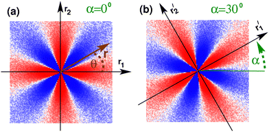
in reciprocal space with  being the Fourier transformed strain tensor field components. (The average 〈…〉 will be specified below) An example for the autocorrelation function c1212(r) of the shear strain ε12(r) is given in Fig. 1 for the same two-dimensional model system already used in ref. 4 and 18. Interestingly, the correlation function is seen to strongly depend both on the orientation of the field vector r (panel (a)) and on the rotation angle α of the coordinate system (panel (b)). Since the simulated system can be shown to be perfectly isotropic down to a few particle diameters,4,18,36–39 these findings beg for an explanation. Expanding on our recent work on stress correlations,4,17,18 this behavior can be traced back to the fact that correlation functions of tensor fields of isotropic systems must be components of a generic isotropic tensor field (cf. Section IIB). This field is shown below (cf. Section IIID) to be completely described in terms of two ICFs cL(q) and cT(q) in reciprocal space (q = |q| being the magnitude of the wavevector). These ICFs characterize the independent fluctuations of the longitudinal and transverse strain components εL(q) and εT(q). Due to the equipartition theorem of statistical physics cL(q) and cT(q) are given by7,10,11,21
| |  | (2) |
in the large-wavelength limit with β = 1/kBT being the inverse temperature, V the d-dimensional volume of the system and λ and μ two macroscopic Lamé coefficients.7,8 All strain correlation functions are thus imposed on large scales. In turn this explains without any additional physical input the octupolar pattern† observed in Fig. 1 (cf. Section IVC and Appendix D) and shows that strain correlations in elastic bodies must necessarily be long-ranged. This is different for the closely related but distinct tensorial response field being the tensorial product of correlation functions and the imposed tensorial perturbation. As emphasized in Sections IIE and V, the response field thus contains additional information due to the source term and its symmetry.
 |
| | Fig. 1 Autocorrelation function c1212(r) of the strain field component ε12(r) obtained from our colloidal glasses in two dimensions: (a) unrotated frame with coordinates (r1, r2), (b) frame  rotated by an angle α = 30° (rotations marked by “′”). Albeit the system is isotropic, the correlation function is strongly angle dependent, revealing an octupolar symmetry. While each pixel corresponds in (a) and (b) to the same spatial position r, the correlation functions differ by the angle α. c1212(r) is positive (red) along the axes and negative (blue) along the bisection lines of the respective axes. rotated by an angle α = 30° (rotations marked by “′”). Albeit the system is isotropic, the correlation function is strongly angle dependent, revealing an octupolar symmetry. While each pixel corresponds in (a) and (b) to the same spatial position r, the correlation functions differ by the angle α. c1212(r) is positive (red) along the axes and negative (blue) along the bisection lines of the respective axes. | |
C. Outline
We begin in Section II with some general theoretical considerations on isotropic tensor fields. Technical points concerning the model system and the data production of tensorial fields on discrete grids are discussed in Section III. This is followed in Section IV by the presentation of our main numerical results. The strain response due to an imposed stress point source is discussed in Section V. A summary and an outlook are given in Section VI. More details may be found in the Appendix both on the theoretical background (cf. Appendices A and D) and on computational issues (cf. Appendices B and C).
II. General considerations
A. Isotropic tensors and tensor fields
Isotropic systems, such as generic isotropic elastic bodies,7–9 simple and complex fluids,34,40–42 amorphous metals and glasses,23–25,27–32,43 polymer networks and gels,40,41 foams and emulsions20,22 or, as a matter of fact, our entire universe5 are described at least on some scales by isotropic tensors and isotropic tensor fields (cf. Appendix A2).1,3,9 It is well known3,9 that the components of isotropic tensors remain unchanged under an orthogonal coordinate transformation (including rotations and reflections). For instance,| |  | (3) |
for the forth-order elastic modulus tensor of an isotropic body (cf. Appendix C3)8,9 with “*” marking an arbitrary orthogonal transformation (cf. Appendix A1). This implies (cf. Appendix A4) that Eαβγδ is given by two invariants, e.g., the two Lamé coefficients λ and μ. Importantly, this does not hold for isotropic tensor fields.3,4,17 For instance, for a forth-order correlation function in reciprocal space the isotropy condition becomes| |  | (4) |
with q* being the “actively” transformed wavevector (cf. Appendix A2).
B. Structure of isotropic correlation functions
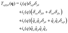
Assuming in addition the system to be achiral and two-dimensional (cf. Appendix A3) it can be shown4 that correlation functions of second-order tensor field components must take the following mathematical structure| | 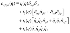 | (5) |
in terms of four ICFs in(q), the coordinates ![[q with combining circumflex]](https://www.rsc.org/images/entities/i_char_0071_0302.gif) α of the normalized wavevector
α of the normalized wavevector ![[q with combining circumflex]](https://www.rsc.org/images/entities/b_char_0071_0302.gif) and the Kronecker symbol δαβ. Legitimate correlation functions of isotropic systems may thus depend on
and the Kronecker symbol δαβ. Legitimate correlation functions of isotropic systems may thus depend on ![[q with combining circumflex]](https://www.rsc.org/images/entities/i_char_0071_0302.gif) α and, hence, on the orientation of the wavevector and of the coordinate system. While the isotropy of the system may not be manifested by one correlation function, it is crucial for the structure of the complete set of all correlation functions given by eqn (5). We note finally that it is useful to express the above ICFs in terms of an alternative set of ICFs cL(q), cT(q), c⊥(q) and cN(q) given by
α and, hence, on the orientation of the wavevector and of the coordinate system. While the isotropy of the system may not be manifested by one correlation function, it is crucial for the structure of the complete set of all correlation functions given by eqn (5). We note finally that it is useful to express the above ICFs in terms of an alternative set of ICFs cL(q), cT(q), c⊥(q) and cN(q) given by| |  | (6) |
See Appendix A4 for more details.
C. Planar harmonic basis functions
Instead of using the components ![[q with combining circumflex]](https://www.rsc.org/images/entities/i_char_0071_0302.gif) α one may, quite generally, express all isotropic tensor fields in two dimensions in terms of the orthogonal planar harmonic basis functions cos(pθ) and sin(pθ) with
α one may, quite generally, express all isotropic tensor fields in two dimensions in terms of the orthogonal planar harmonic basis functions cos(pθ) and sin(pθ) with ![[q with combining circumflex]](https://www.rsc.org/images/entities/i_char_0071_0302.gif) 1 = cos(θ) and
1 = cos(θ) and ![[q with combining circumflex]](https://www.rsc.org/images/entities/i_char_0071_0302.gif) 2 = sin(θ) and p = 0, 2 and 4. (See Appendix D for more details.) For instance, it follows from eqn (5) that
2 = sin(θ) and p = 0, 2 and 4. (See Appendix D for more details.) For instance, it follows from eqn (5) that| |  | (7) |
Hence, if the invariant i4(q) is sufficiently large, c1212(q) must reveal an octupolar pattern. Due to eqn (B18) derived in Appendix B3, this alternative representation is especially useful for performing the inverse FT to real space. This also shows that the corresponding correlation function  in real space must have the same mathematical properties.
D. Response to point source
Let us consider the second order tensor field Rαβ(q) obtained by the contraction| |  | (8) |
with a symmetric but not necessarily isotropic tensor sαβ using the standard summation convention over repeated indices.1,3 (For convenience we have introduced the system volume V.) We shall call Rαβ(q) the “response field” (in reciprocal space) and sαβ the “point source tensor”. In fact, using eqn (B4) and (B6) it is seen that in real space the tensor sαβ/V corresponds to a “point source” sαβδ(r) (using Dirac's delta function) and Rαβ(q) becomes| |  | (9) |
using  . We shall say more about the specific linear strain response in real space in Section V but focus here on the generic response in reciprocal space. Being symmetric the source tensor may be diagonalized by a rotation of the coordinate system where s12 = s21 = 0 and s11 and s22 become the two (in general not identical) eigenvalues. Hence,
| |  | (10) |
We emphasize that the sum must be taken over all eigenvalues of the source tensor, i.e. two for the presented two-dimensional case. (The failure to sum properly over all tensorial contributions to Rαβ(q) leads to incorrect angular dependences.) Importantly, Rαβ(q) thus contains information over both the system, characterized by the correlation functions, and the imposed source term.
E. Different types of source terms
If we now assume that not only cαβγδ(q) is an isotropic tensor field but that, moreover, sαβ is isotropic, i.e. s11 = s22, the product theorem eqn (A7) discussed in Appendix A2 implies that Rαβ(q) must also be an isotropic tensor field. According to eqn (A15) it is given by| | Rαβ(q) = k1(q)δαβ + k2(q)![[q with combining circumflex]](https://www.rsc.org/images/entities/i_char_0071_0302.gif) α α![[q with combining circumflex]](https://www.rsc.org/images/entities/i_char_0071_0302.gif) β β | (11) |
in terms of two invariants k1(q) and k2(q) which can in turn be expressed in terms of the invariants of cαβγδ(q) and sαβ. Rαβ(q) can thus at most be quadrupolar (p = 2). Specifically,| | R12(q) = k2(q)![[q with combining circumflex]](https://www.rsc.org/images/entities/i_char_0071_0302.gif) 1 1![[q with combining circumflex]](https://www.rsc.org/images/entities/i_char_0071_0302.gif) 2 ∝ sin(2θ) 2 ∝ sin(2θ) | (12) |
which is distinct from c1212(q), cf.eqn (7). Importantly, in many physical situations the source is in fact not isotropic and thus in turn the response field not consistent with eqn (11). We remind that according to a popular model of localized plastic failure by means of “shear transformation zones”23,44–47 two orthogonal twin force dipoles of opposite signs may be imposed at the origin.‡ This suggests to consider the case s11 = −s22. It follows then from eqn (5) and (10) that| | R12(q) ∝ i4(q)![[q with combining circumflex]](https://www.rsc.org/images/entities/i_char_0071_0302.gif) 1 1![[q with combining circumflex]](https://www.rsc.org/images/entities/i_char_0071_0302.gif) 2( 2(![[q with combining circumflex]](https://www.rsc.org/images/entities/i_char_0071_0302.gif) 12 − 12 − ![[q with combining circumflex]](https://www.rsc.org/images/entities/i_char_0071_0302.gif) 22) ∝ sin(4θ). 22) ∝ sin(4θ). | (13) |
The (non-isotropic) response field R12(q) thus is in this case octupolar as the correlation field c1212(q), however, shifted by an angle π/8. It is readily seen by inverse FT that the same general behavior applies in real space.
III. Technical issues
A. Algorithm, configurations and frames
We investigate amorphous glasses in two dimensions formed by pLJ particles4,18,36–39,48 which are sampled by means of Monte Carlo (MC) simulations.33 See Appendix C for details (Hamiltonian, units, cooling and equilibration procedure, data production, generation and analysis of tensor fields on discrete grids). We focus on systems containing n = 10![[thin space (1/6-em)]](https://www.rsc.org/images/entities/char_2009.gif) 000 and 40
000 and 40![[thin space (1/6-em)]](https://www.rsc.org/images/entities/char_2009.gif) 000 particles at a working temperature T = 0.2. This is much lower than the glass transition temperature Tg ≈ 0.26,36i.e. for any computationally feasible production time the systems behave as solid elastic bodies.38Nc = 200 completely independent configurations c are prepared using a mix of local and swap MC hopping moves38,49 while the presented data are computed using local MC moves only. For each c we store time-series containing Nt = 10
000 particles at a working temperature T = 0.2. This is much lower than the glass transition temperature Tg ≈ 0.26,36i.e. for any computationally feasible production time the systems behave as solid elastic bodies.38Nc = 200 completely independent configurations c are prepared using a mix of local and swap MC hopping moves38,49 while the presented data are computed using local MC moves only. For each c we store time-series containing Nt = 10![[thin space (1/6-em)]](https://www.rsc.org/images/entities/char_2009.gif) 000 “frames” t computed using equidistant time intervals. As described in Appendix C3, the elastic modulus tensor is isotropic and determined by the two Lamé coefficients λ ≈ 38 and μ ≈ 14.36,38
000 “frames” t computed using equidistant time intervals. As described in Appendix C3, the elastic modulus tensor is isotropic and determined by the two Lamé coefficients λ ≈ 38 and μ ≈ 14.36,38
B. Sampled discrete tensorial fields
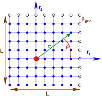
As shown in Fig. 2, a discrete square grid is used to store and to manipulate the various fields needed for the microscopic description. The standard lattice constant for the grid in real space is agrid ≈ 0.2. The displacement field u(r) in real space is determined for each frame t using a standard method10,11,21 from the displacement vector of each particle using as reference position the time-averaged particle position (cf. Appendix C5). We obtain then from the Fourier transformed displacement field  the strain tensor field8,17
| |  | (14) |
in reciprocal space. Using the correlation function theorem for FTs (cf. Appendix B) the strain correlations functions in reciprocal space are given by eqn (1) where the average is taken over all t and c. Both strain and correlation function fields in reciprocal space are defined to be dimensionless (cf. Appendix B1). We emphasize by a prime “′” all tensor field components obtained in a coordinate system rotated by an angle α (with α = 0 being the original unrotated system). Specifically, the correlation functions  are obtained using the components
  and
and  in the rotated frame.
 |
| | Fig. 2 Two-dimensional (d = 2) square lattice with agrid being the lattice constant and nL = L/agrid the number of grid points in one spatial dimension. The filled circles indicate microcells of the principal box, the open circles some periodic images. The spatial position r of a microcell is either given by the r1- and r2-coordinates (in the principal box) or by the distance r = |r| from the origin (large circle) and the angle θ. | |
C. Natural Rotated Coordinates
All the tensorial fields introduced above depend on the orientation of the coordinate system. Importantly, we consider these properties in a first step in “Natural Rotated Coordinates” (NRC) where for each wavevector q the coordinate system is rotated until the 1-axis coincides with the q-direction. We mark these new tensor field components by “°” to distinguish them from standard rotated tensor field components (marked by primes “′”). Note that  for all wavevectors q. Using the components
  and
and  we obtain (as before) the strain tensor
  . Importantly,
| |  | (15) |
in agreement with eqn (14). We thus only have two independent components of the strain tensor field in NRC. We alternatively write for convenience  ,
,  ,
,  and
and  for the longitudinal and transverse components of the displacement and strain tensor fields. Note that
| |  | (16) |
and| |  | (17) |
i.e. displacement and strain fields in NRC contain essentially the same information.
D. Correlation functions in NRC
The correlation functions  may for finite Nc not only depend on q but also on
 ![[q with combining circumflex]](https://www.rsc.org/images/entities/b_char_0071_0302.gif) . Consistently with eqn (A18) and ref. 4, 17 and 18 we thus operationally define the ICFs
. Consistently with eqn (A18) and ref. 4, 17 and 18 we thus operationally define the ICFs  ,
,  ,
,  and
and  by averaging over all wavevectors with |q| ≈ q. However,
  implies immediately that
| |  | (18) |
The two remaining non-trivial ICFs cL(q) and cT(q) are called, respectively, the “longitudinal ICF” and the “transverse ICF”. As already noted in the Introduction, according to the equipartition theorem cL(q) and cT(q) are given for sufficiently large wavelengths by the Lamé coefficients λ and μ. The stated eqn (2) can be readily obtained from published work7,10,11,21 using eqn (16) and (17) to substitute the displacement fields uL(q) and uT(q) in NRC by the corresponding strain fields εL(q) and εT(q).
IV. Main numerical results
A. Measured longitudinal and transverse ICFs
We turn now to the numerical results of this work. Fig. 3 focuses on the two non-vanishing correlation functions obtained in reciprocal space and NRC. All correlation functions are rescaled by βV having thus the dimension of an inverse modulus. As can be seen for the two indicated particle numbers n, a data collapse for different system sizes is observed, confirming the expected volume scaling. The inset presents the (not yet spherically averaged) correlation functions  and
and  as functions of the wavevector angle θ for one small wavevector with q ≈ 0.1. As expected for isotropic systems, these correlation functions are θ-independent (apart from a small noise contribution due to the finite number of independent configurations). The main panel presents the
 ![[q with combining circumflex]](https://www.rsc.org/images/entities/i_char_0071_0302.gif) -averaged longitudinal and transverse ICFs βVcL(q) and βVcT(q) as functions of q. The expected large-wavelength limit eqn (2) is indicated in both panels by bold horizontal lines. As can be seen in the main panel, it is well confirmed for q ≪ 1 over at least one order of magnitude where we have used the known values of λ and μ. We remind that eqn (2) has been used in various experimental and numerical studies10,11,21 to fit λ and μ. cL(q) and cT(q) characterize the typical length of the complex random variables εL(q) and εT(q). Their distributions and correlations will be discussed elsewhere.50 We note finally that the increase of the ICFs from the low-q asymptotics visible for q > 1 correlates with the deviation of the total static structure factor S(q) from its low-q plateau (cf.Fig. 6).
-averaged longitudinal and transverse ICFs βVcL(q) and βVcT(q) as functions of q. The expected large-wavelength limit eqn (2) is indicated in both panels by bold horizontal lines. As can be seen in the main panel, it is well confirmed for q ≪ 1 over at least one order of magnitude where we have used the known values of λ and μ. We remind that eqn (2) has been used in various experimental and numerical studies10,11,21 to fit λ and μ. cL(q) and cT(q) characterize the typical length of the complex random variables εL(q) and εT(q). Their distributions and correlations will be discussed elsewhere.50 We note finally that the increase of the ICFs from the low-q asymptotics visible for q > 1 correlates with the deviation of the total static structure factor S(q) from its low-q plateau (cf.Fig. 6).
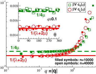 |
| | Fig. 3 Rescaled correlation functions in NRC and reciprocal space. The bold dashed and solid lines indicate the expected low-q limit eqn (2). Inset:  and and  vs. θ for q ≈ 0.1. Main panel: Semi-logarithmic representation of ICFs βVcT(q) and βVcL(q) vs. q. vs. θ for q ≈ 0.1. Main panel: Semi-logarithmic representation of ICFs βVcT(q) and βVcL(q) vs. q. | |
B. Correlation functions in reciprocal space
While remaining in reciprocal space we consider next coordinate frames which are either unrotated (α = 0) or rotated as in Fig. 1(b) using the same angle α for all q. According to eqn (5) the correlation functions cαβγδ(q) of isotropic achiral systems in two dimensions depend quite generally on the four ICFs cL(q), cT(q), cN(q) and c⊥(q). Due to eqn (18) the last two of these ICFs must vanish while cL(q) and cT(q) are given by eqn (2). Let us introduce for later convenience the two “creep compliances”| |  | (19) |
This yields in the original coordinates| |  | (20) |
| |  | (21) |
| |  | (22) |
| |  | (23) |
for q → 0. The dots mark irrelevant constant contributions.§ See Appendix D for more details. For correlation functions  in rotated coordinate systems one merely needs to substitute θ by x = θ − α. These relations are put to a test in Fig. 4 where we focus for clarity on the reduced shear-strain autocorrelation function
  for n = 40
![[thin space (1/6-em)]](https://www.rsc.org/images/entities/char_2009.gif) 000. The angular dependences are presented in the main panel for one wavevector in the low-q limit. Focusing on the first term in eqn (20) we have taken off the mean constant average over all θ (corresponding to the dots). Importantly, all data for different α are seen to collapse when plotted as a function of the scaling variable x. Obviously, this simple scaling (without characteristic angle) would not hold for anisotropic systems. To obtain a precise test of the q-dependence of cαβγδ(q) we project out the angular dependences using
000. The angular dependences are presented in the main panel for one wavevector in the low-q limit. Focusing on the first term in eqn (20) we have taken off the mean constant average over all θ (corresponding to the dots). Importantly, all data for different α are seen to collapse when plotted as a function of the scaling variable x. Obviously, this simple scaling (without characteristic angle) would not hold for anisotropic systems. To obtain a precise test of the q-dependence of cαβγδ(q) we project out the angular dependences using| |  | (24) |
for p = 2 and p = 4. For convenience the prefactor of the integral is chosen such that P[cos(2θ),2] = P[cos(4θ),4] = 1. The result for the shear-stress autocorrelation function with p = 4 is shown in the inset of Fig. 4. In agreement with eqn (20) the presented data is given by J1/8 (solid line) for sufficiently small wavevectors. Equivalent results have been obtained for the other correlation functions mentioned above.
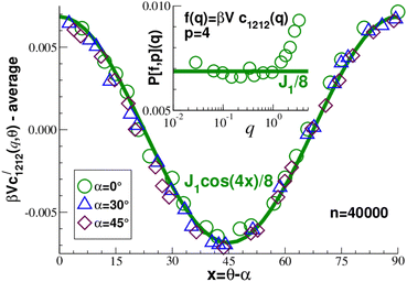 |
| | Fig. 4 Rescaled correlation function  for n = 40 for n = 40![[thin space (1/6-em)]](https://www.rsc.org/images/entities/char_2009.gif) 000. Main panel: Angle dependence of vertically shifted f(q) for q ≈ 0.1. Data collapse is observed using the reduced angle x = θ−α. The bold solid line indicates the prediction, eqn (20). Inset: Comparison of P[f,p](q) for p = 4 with the predicted low-q limit J1/8 (bold solid line). 000. Main panel: Angle dependence of vertically shifted f(q) for q ≈ 0.1. Data collapse is observed using the reduced angle x = θ−α. The bold solid line indicates the prediction, eqn (20). Inset: Comparison of P[f,p](q) for p = 4 with the predicted low-q limit J1/8 (bold solid line). | |
C. Correlation functions in real space
We turn finally to the correlation functions  in real space. As shown in Appendix D, inverse FT implies
| |  | (25) |
with x = θ − α being the difference of the angles θ and α indicated in Fig. 1. The same large-r limit holds also for  and for
  . Moreover,
| |  | (26) |
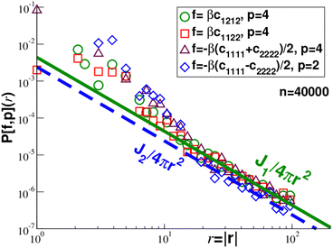
for r ≫ 1, i.e. a dipolar symmetry is expected. A verification of the r-dependence is obtained using again (now in real space) the projection P[f,p](r), cf.eqn (24). Focusing on n = 40![[thin space (1/6-em)]](https://www.rsc.org/images/entities/char_2009.gif) 000 several rescaled correlation functions f(r) are presented in Fig. 5. In agreement with eqn (25) the indicated first three cases collapse for p = 4 and r ≳ 20 on J1/4πr2 (bold solid line). This confirms the octupolar symmetry of these correlation functions. Confirming eqn (26) the last case with f(r) = −β(c1111(r) − c2222(r))/2 collapses onto J2/4πr2 (dashed line). p = 2 is used here in agreement with the predicted quadrupolar symmetry of this correlation function. Similar results are obtained for other particle numbers n.
000 several rescaled correlation functions f(r) are presented in Fig. 5. In agreement with eqn (25) the indicated first three cases collapse for p = 4 and r ≳ 20 on J1/4πr2 (bold solid line). This confirms the octupolar symmetry of these correlation functions. Confirming eqn (26) the last case with f(r) = −β(c1111(r) − c2222(r))/2 collapses onto J2/4πr2 (dashed line). p = 2 is used here in agreement with the predicted quadrupolar symmetry of this correlation function. Similar results are obtained for other particle numbers n.
 |
| | Fig. 5
P[f,p](r) for various correlation functions and modes p for n = 40![[thin space (1/6-em)]](https://www.rsc.org/images/entities/char_2009.gif) 000. The bold solid line marks the prediction J1/4πr2 for the first three cases, the dashed line the prediction J2/4πr2 for the last one. 000. The bold solid line marks the prediction J1/4πr2 for the first three cases, the dashed line the prediction J2/4πr2 for the last one. | |
V. Linear response to point stress
A. Time-dependent strain correlations
Correlation functions describe quite generally the linear response to a small imposed perturbation.7,34,35,42 Being tensorial fields, just like the correlation function fields, the response fields must in general depend on the direction of the field vector and on the orientation of the coordinate system. As already emphasized in Section II4 and Section II5, the response fields contains information of both the system and the imposed source and the source term may either be isotropic or anisotropic. We elaborate here this general point focusing, naturally, on correlation functions of the instantaneous strain field ![[small epsilon, Greek, circumflex]](https://www.rsc.org/images/entities/i_char_e107.gif) αβ(r) = εαβ(r, t). Extending very briefly our discussion to the time domain, let us introduce the time-dependent correlation functions
αβ(r) = εαβ(r, t). Extending very briefly our discussion to the time domain, let us introduce the time-dependent correlation functions| | | cαβγδ(q, t) = 〈εαβ(q, t)εγδ(−q, t = 0)〉 | (27) |
of the strain fields in reciprocal space with t being the “time lag”.33 Naturally, this reduces to eqn (1) for t → 0. This definition allows us to take advantage of the general “Fluctuation-dissipation theorem” (FDT) of statistical mechanics as stated, e.g., in ref. 34, 35 and 42. We thus anticipate immediate generalizations of the present study for time-dependent tensorial correlation and response fields which will be discussed elsewhere.
B. Fluctuation-dissipation theorem
Let us switch on at time t = 0 a small perturbation| |  | (28) |
to the Hamiltonian  of the system with δσαβ(r) being an imposed external stress field. This is equivalent to the application of an appropriate external perturbative force field to each particle. For a general “growth function”42 in response to a sudden application of a step field, such as eqn (28), the relevant FDT relations are stated (for scalar fields) by eqn (3.65) and (3.67) of ref. 42. The mean strain increment δεαβ(r, t) induced by this perturbation is then given in real space by a convolution integral for the time-dependent correlation functions cαβγδ(r, t) and the stress perturbation δσαβ(r). Using eqn (B6) this relation may be written more compactly in reciprocal space as
| | | δεαβ(q, t) = βV [cαβγδ(q, t = 0) − cαβγδ(q, t)]δσγδ(q) | (29) |
where the summation over repeated indices is essential and cannot be omitted. Note that δεαβ(q, t) = 0 for t ≤ 0 and that, since all cαβγδ(q, t) are continuous functions of time, the creep response δεαβ(q, t) must also be continuous, especially at t = 0.40 The time-dependent creep is thus determined by the time-dependent correlation functions and the imposed stress perturbation. We are interested here only in the static equilibrium response a long time after the perturbation is switched on. The time-dependent strain correlation functions (computed for the unperturbed Hamiltonian  at switched off external perturbation
  ) must, of course, vanish
| | | cαβγδ(q, t) → 0 for t → ∞. | (30) |
Hence, eqn (29) reduces to| | | δεαβ(q) = βVcαβγδ(q)δσγδ(q) for t → ∞ | (31) |
with  denoting the long-time creep and
  standing for the spatial correlation function without time lag, eqn (1), as everywhere else in this paper.
C. Response to point source
Following the discussion at the end of Section II, we investigate now the long-time creep for a point sourcewith sαβ being a symmetric 2 × 2 matrix (of dimension “stress × volume = energy”). According to the FDT relation eqn (31) this implies| | | δεαβ(q) = βcαβγδ(q)sγδ for t → ∞ | (33) |
and an equivalent relation in real space. As in Section IID it is convenient to diagonalize sαβ by an appropriate rotation of the coordinate system. The perturbation becomes therefore equivalent to that of two small force dipoles23 oriented along the eigenvectors. The real-space analogue of eqn (10) is thus given by| | | δεαβ(r) = βcαβ11(r)s11 + βcαβ22(r)s22. | (34) |
Using in addition eqn (D13) we may replace for isotropic systems the real space correlation functions by the corresponding invariants ĩn(r) in real space. Introducing the scalars s1 = sγγ/2 and s2 = ![[r with combining circumflex]](https://www.rsc.org/images/entities/i_char_0072_0302.gif) αsαβ
αsαβ![[r with combining circumflex]](https://www.rsc.org/images/entities/i_char_0072_0302.gif) β/2 this may be written quite generally
β/2 this may be written quite generally| |  | (35) |
Taking now advantage of the specific results for strain correlations presented in Section IVC and in Appendix D the invariants ĩn(r) are given by eqn (D14), i.e. we may quite generally express δεαβ(r) in terms of the two creep compliances J1 and J2, cf.eqn (19).
We also note that the term sαβ in the last line of eqn (35) must be isotropic, i.e. s1 = s11 = s22 = 2s2, to obtain an isotropic second-order tensor field in agreement with eqn (A20). As expected from the more general argument given in Section 2, the shear strain increment
| |  | (36) |
becomes quadrupolar in this case.
As already emphasized in Section IIE, the source tensor need not necessarily be isotropic albeit the system is isotropic. To be specific, let us consider the “shear transformation zone” model for localized plastic failure involving two orthogonal force dipoles of opposite signs.23 Hence, s11 = −s22 and s1 = 0 and s2 = s11(![[r with combining circumflex]](https://www.rsc.org/images/entities/i_char_0072_0302.gif) 12 −
12 − ![[r with combining circumflex]](https://www.rsc.org/images/entities/i_char_0072_0302.gif) 22)/2. Using eqn (13) or eqn (35) this yields
22)/2. Using eqn (13) or eqn (35) this yields
| |  | (37) |
for the shear strain response.
As one expects on general grounds, all reference to statistical physics, i.e. the inverse temperature β, drops out in both cases. Moreover, the shear strain response naturally strongly depends on the type of source term applied at the origin: for force dipoles of same sign it is quadrupolar and proportional to J2 while for dipoles of opposite sign it gets octupolar and proportional to J1.
VI. Conclusion
A. Summary
Strain correlation functions.
The present work has focused on correlation functions of components of strain tensor fields in two-dimensional, isotropic and achiral elastic bodies. This was done theoretically using
• the general mathematical structure of isotropic tensor fields as summarized in Section IIB, cf.eqn (5), and in more detail in Appendix A and
• the well-known equipartition theorem of statistical physics for macroscopic strain fluctuations in reciprocal space, cf.eqn (2).
Numerically we have tested our predictions by means of glass-forming particles deep in the glass regime. This shows that these correlation functions may depend on the coordinates of the field variable (qα in reciprocal space or rα in real space) and implies in turn that they depend in general on the direction of the field vector and on the orientation of the coordinate system. Scaling with x = θ − α these angular dependencies are distinct from those of ordinary anisotropic systems. Importantly, correlation functions of strain tensor fields are components of an isotropic forth-order tensor field, eqn (5), being characterized by the two ICFs cL(q) and cT(q). With the asymptotic plateau values being given by two Lamé coefficients, eqn (2), all strain correlation functions are determined and all (finite) real-space strain correlations must be long-ranged decaying as 1/r2 (cf.Fig. 5). We thus obtain similar results as in our recent study on correlation functions of stress tensor fields.4 Note that time-averaged stress fields have been probed in the latter study while correlations of instantaneous strain fields have been considered here. Our numerical findings do agree with other studies of strain correlations29,30,32 being, however, now traced back to the isotropy of the system and the tensor field nature of the probed correlations. Importantly, we have given here a complete and asymptotically exact description for the correlation functions of strain tensor fields of isotropic elastic bodies. No additional physical assumption is thus needed (for sufficiently small wavevectors).
Response to tensorial point sources.
We also discussed the associated linear response fields as defined in general mathematical terms by the tensorial contraction of the correlation function tensor by means of a source tensor and, more physically, by the FDT relation for the strain increment due to an imposed small stress perturbation, cf.eqn (28) and (29). Naturally, the response must by definition contain information from both the correlation functions, characterizing the system, and from the imposed source tensor which may not be isotropic. We have emphasized that the summation over repeated indices must be properly performed, i.e. the response field is not given by one correlation function times a scalar but by the sum over all eigenvalues of the source tensor. For this reason response and correlation fields, albeit closely related, have in general different angular dependences, e.g., the shear strain correlation function c1212(r) in an isotropic system must be octupolar, cf.eqn (25), while the shear strain response δε12(r) may be either quadrupolar for an isotropic source, cf.eqn (36), or octupolar for an anisotropic source corresponding to two force dipoles of opposite signs, cf.eqn (37). Albeit all contributing correlation functions are isotropic the response field is anisotropic in the latter case due to the source. It is thus important to not lump together correlation functions and response fields. Mesoscopic elasto-plastic models45,46 thus must specify not only the correlation functions but also the source tensors characterizing the local plastic events.
B. Outlook
Our work suggests several natural extensions:
• The general mathematical framework for isotropic tensor fields and the discussed relations and numerical procedure for correlation and response fields naturally generalize to higher spatial dimensions, especially for the three-dimensional case.
• The present work has focused on Euclidean spaces and Cartesian coordinates. A generalization for systems embedded in non-Euclidean spaces, say for glasses on spheres,51,52 and more general curvilinear coordinate systems1,5 may be worked out.
• The present work has focused on the large-wavelength limit (q → 0). More generally, one may express the longitudinal and transverse ICFs cL(q) and cT(q) for finite q as
| |  | (38) |
in terms of the generalized longitudinal and transverse elastic moduli
L(
q) and
G(
q) (with
L(
q) →
λ + 2
μ and
G(
q) →
μ for small
q).
¶![[thin space (1/6-em)]](https://www.rsc.org/images/entities/char_2009.gif) 17,48,50
17,48,50 It can be shown
50 that both the isotropicity and the harmonicity of the strain modes assumed in the derivation of
eqn (38) are well justified for the present model up to
q ≈ 1 while deviations become relevant for larger wavevectors, especially around the main peak of the static structure factor
S(
q).
• A further generalization of the current work concerns time-dependent correlation functions cαβγδ(q, t) as defined in eqn (27). These can be again expressed viaeqn (5) in terms of (now time-dependent) longitudinal and transverse ICFs cL(q, t) and cT(q, t). These time-dependent ICFs are given in turn by time-dependent creep compliance material functions which can be related to the two time-dependent material functions L(q, t) and G(q, t).17 Strain correlation functions may thus reveal octupolar pattern whenever the invariant
| | | |i4(q, t)| = |cL(q, t) − 4cT(q, t)| | (39) |
is sufficiently large. Since
i4(
q,
t) must become
q-independent for small
q, a long-range decay with
is generally expected for the time-dependent correlation functions in isotropic
d-dimensional systems. Using
eqn (29) similar long-range relations are predicted for the associated dynamical response fields.
• It may be also of interest to characterize correlations of tensor fields of different order. For instance, the forth-order elastic modulus field Eαβγδ(r)26,53 may be characterized by a correlation function tensor of order eight.53 Strong angular dependencies are expected based on our formalism. For isotropic systems these correlation functions must again adopt a general mathematical structure in terms of a small finite number of ICFs. Once these ICFs are characterized (theoretically or numerically using NRC) in the low-q limit all correlation functions are again determined.
Author contributions
J. P. W. designed and wrote the project benefitting from contributions of all co-authors.
Conflicts of interest
There are no conflicts to declare.
Appendix A Summary of isotropic tensor fields
1 Background
Isotropic systems are described by “isotropic tensors” and “isotropic tensor fields”. We give here a brief recap of various useful aspects already presented elsewhere.3,4 Quite generally, a tensor field assigns a tensor to each point of the mathematical space, in our case a d-dimensional Euclidean vector space.3 We denote an element of this vector space by the “spatial position” r (real space) or by the “wavevector” q for the corresponding reciprocal space. The relations for tensor fields are formulated in reciprocal space since this is more convenient both on theoretical and numerical grounds due to the assumed spatial homogeneity (“translational invariance”). The corresponding real space tensor field is finally obtained by inverse FT.
For simplicity we assume Cartesian coordinates with an orthonormal basis {e1,…, ed}.1,3,9 Greek letters α, β, … are used for the indices of the tensor (field) components. A twice repeated index α is summed over the values 1, …, d, e.g., q = qαeα with qα standing for the vector coordinates. This work is chiefly concerned with tensors T(o) = Tα1…αoeα1… eαo of “order” o = 2 and o = 4 and their corresponding tensor fields with components depending either on r or q. The order of a component is given by the number of indices. Note that
| |  | (A1) |
for the
do coordinates in real and reciprocal space (with

denoting the FT as discussed in Appendix B).
We consider linear orthogonal coordinate transformations (marked by “*”)  with matrix coefficients cαβ given by the direction cosine
  .3 We remind that3
| |  | (A2) |
under a general orthogonal transform. For a reflection of the 1-axis we thus have,
e.g.,
| |  | (A3) |
i.e. we have sign inversion for an odd number of indices equal to the index of the inverted axis. The field vector

remains unchanged by these “passive” transforms albeit its coordinates change.
2 Definitions, properties and construction of general isotropic tensors and tensor fields
Isotropic tensors.
Components of an isotropic tensor remain unchanged by any orthogonal coordinate transformation,3,9i.e.| |  | (A4) |
As noted at the end of Section A1 the sign of tensor components change for a reflection at one axis if the number of indices equal to the inverted axis is odd. Consistency with eqn (A4) implies that all tensor components with an odd number of equal indices must vanish, e.g.,| | | T12 = T1112 = T1222 = 0. | (A5) |
Isotropic tensor fields.
The corresponding isotropy condition for tensor fields is given by3| |  | (A6) |
with  which reduces to eqn (A4) for q = 0. Please note that the fields on the left handside of eqn (A6) are evaluated with the original coordinates of the vector field variable q while the fields on the right handside are evaluated with the transformed coordinates. Another way to state this is to say that the left hand fields are computed at the original vector q = (q1,…,qd) while the right hand fields are computed at the “actively transformed” vector
  . It is for this reason that finite components with an odd number of equal indices, e.g., T1222(q) ≠ 0, are possible in principle for finite q.
Natural rotated coordinates.
Fortunately, there is a convenient coordinate system where the nice symmetry eqn (A5) for isotropic tensors can be also used for isotropic tensor fields. In these “Natural Rotated Coordinates” (NRC) the coordinate system for each wavevector q is rotated until the 1-axis coincides with the q-direction, i.e. with q = |q|. These tensor field components in NRC are marked by “°” to distinguish them from standard rotated tensor fields (marked by primes “′”) where the same rotation is used for all q. If in addition
  is an even function of its field variable q (as in the case of achiral systems for even order o) it can be shown4 that all tensor field components with an odd number of equal indices must vanish.
Product theorem for isotropic tensor fields.
Let us consider a tensor field C(q) = A(q) ⊗ B(q) with A(q) and B(q) being two isotropic tensor fields and ⊗ standing either for an outer product, e.g. cαβγδ(q) = Aαβ(q)Bγδ (q), or an inner product, e.g. cαβγδ(q) = Aαβγν(q)Bνδ(q). Hence,| |  | (A7) |
using in the second step a general property of tensor (field) products, due to eqn (A2), and in the third step eqn (A6) for the fields A(q) and B(q) where q* stands for the “actively” transformed field variable. C(q) is thus also an isotropic tensor field. One may use this theorem to construct isotropic tensor fields from known isotropic tensor fields A(q) and B(q).
3. Summary of assumed symmetries
All second-order tensors in this work are symmetric, Tαβ = Tβα, and the same applies for the corresponding tensor fields in either r- or q-space. This is, e.g., the case for the strain field  , cf.eqn (14), or the source tensor sαβ needed for a response field, cf.eqn (8). We assume for all forth-order tensor fields that
| | | Tαβγδ(q) = Tβαγδ(q) = Tαβδγ(q) | (A8) |
and| | | Tαβγδ(q) = Tαβγδ(−q). | (A10) |
Note that eqn (A10) is necessarily valid both for achiral and chiral two-dimensional isotropic systems. Forth-order tensor fields are often constructed by taking outer products9 of second-order tensor fields. We consider, e.g., correlation functions 〈![[T with combining circumflex]](https://www.rsc.org/images/entities/i_char_0054_0302.gif) αβ(q)
αβ(q)![[T with combining circumflex]](https://www.rsc.org/images/entities/i_char_0054_0302.gif) γδ(−q)〉 with
γδ(−q)〉 with ![[T with combining circumflex]](https://www.rsc.org/images/entities/i_char_0054_0302.gif) αβ(q) being an instantaneous second-order tensor field. eqn (A8) then follows from the symmetry of the second-order tensor fields. The evenness of forth-order tensor fields, eqn (A10), is a necessary condition for achiral systems. It implies that Tαβγδ(q) is real if Tαβγδ(r) is real and, moreover, eqn (A9) for correlation functions since
αβ(q) being an instantaneous second-order tensor field. eqn (A8) then follows from the symmetry of the second-order tensor fields. The evenness of forth-order tensor fields, eqn (A10), is a necessary condition for achiral systems. It implies that Tαβγδ(q) is real if Tαβγδ(r) is real and, moreover, eqn (A9) for correlation functions since| | 〈![[T with combining circumflex]](https://www.rsc.org/images/entities/i_char_0054_0302.gif) αβ(q) αβ(q)![[T with combining circumflex]](https://www.rsc.org/images/entities/i_char_0054_0302.gif) γδ(−q)〉 = 〈 γδ(−q)〉 = 〈![[T with combining circumflex]](https://www.rsc.org/images/entities/i_char_0054_0302.gif) γδ(q) γδ(q)![[T with combining circumflex]](https://www.rsc.org/images/entities/i_char_0054_0302.gif) αβ(−q)〉. αβ(−q)〉. | (A11) |
As already emphasized, all our systems are assumed to be isotropic, i.e., eqn (A6) must hold for ensemble-averaged tensor fields.
4. General mathematical structure
General structure of tensors.
Isotropic tensors of different order are discussed, e.g., in Section 2.5.6 of ref. 9. Due to eqn (A5) all such tensors of odd order must vanish. The finite isotropic tensors of lowest order are thus| | | Tαβγδ = i1δαβδγδ + i2(δαγδβδ + δαδδβγ) | (A13) |
with k1, i1 and i2 being invariant scalars. Please note that all symmetries stated above hold, especially also eqn (A5). Note that the symmetry eqn (A8) was used for the second relation, eqn (A13). Importantly, this implies that only two coefficients are needed for a forth-order isotropic tensor. As a consequence, the elastic modulus tensor is completely described by two elastic moduli (cf. Section 9.3).
General structure of tensor fields.
We restate now the most general isotropic tensor fields for 1 ≤ o ≤ 4 and focusing on two-dimensional systems (d = 2) compatible with the symmetries stated in Section 7.3. With ln(q), kn(q), jn(q) and in(q) being invariant scalar functions of q = |q| we have3,4| | Tα(q) = l1(q)![[q with combining circumflex]](https://www.rsc.org/images/entities/i_char_0071_0302.gif) α α | (A14) |
| | Tαβ(q) = k1(q)δαβ + k2(q)![[q with combining circumflex]](https://www.rsc.org/images/entities/i_char_0071_0302.gif) α α![[q with combining circumflex]](https://www.rsc.org/images/entities/i_char_0071_0302.gif) β β | (A15) |
| | Tαβγ(q) = j1(q)![[q with combining circumflex]](https://www.rsc.org/images/entities/i_char_0071_0302.gif) αδβγ + j2(q) αδβγ + j2(q)![[q with combining circumflex]](https://www.rsc.org/images/entities/i_char_0071_0302.gif) βδαγ + j3(q) βδαγ + j3(q)![[q with combining circumflex]](https://www.rsc.org/images/entities/i_char_0071_0302.gif) γδαβ + j4(q) γδαβ + j4(q)![[q with combining circumflex]](https://www.rsc.org/images/entities/i_char_0071_0302.gif) α α![[q with combining circumflex]](https://www.rsc.org/images/entities/i_char_0071_0302.gif) β β![[q with combining circumflex]](https://www.rsc.org/images/entities/i_char_0071_0302.gif) γ γ | (A16) |
| |  | (A17) |
for finite wavevectors q. See ref. 4 for a derivation, generalizations for d > 2 and a discussion of the limit q → 0. Terms due to the invariants k1(q), i1(q) and i2(q) are independent of the coordinate system. All other terms depend on the components ![[q with combining circumflex]](https://www.rsc.org/images/entities/i_char_0071_0302.gif) α of the normalized wavevector
α of the normalized wavevector ![[q with combining circumflex]](https://www.rsc.org/images/entities/b_char_0071_0302.gif) and thus on the orientations of the field vector and of the coordinate system.
and thus on the orientations of the field vector and of the coordinate system.
Alternative representation for forth-order tensor fields.
It is convenient to define the four functions| |  | (A18) |
using NRC. For an isotropic system these four functions can only depend on the wavenumber q but not on the direction ![[q with combining circumflex]](https://www.rsc.org/images/entities/b_char_0071_0302.gif) of the wavevector q. Importantly, all other components
of the wavevector q. Importantly, all other components  are either by eqn (A8) and (A9) identical to these invariants or must vanish for an odd number of equal indices as reminded in Section A2. The d4 = 16 components
  are thus completely determined by the four invariants and this for any q. Tαβγδ(q) is then obtained by the inverse rotation to the original unrotated frame using eqn (A2). It is readily seen that
| |  | (A19) |
being consistent with eqn (6).
Isotropic tensor fields in real space.
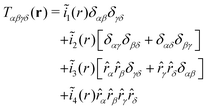
We have formulated above all tensor fields in terms of the wavevector q and its components since it is most convenient to start the analysis in reciprocal space. The above results also hold, however, in real space. This implies, e.g., for isotropic (and achiral) fields in two dimensions that| | Tαβ(r) = ![[k with combining tilde]](https://www.rsc.org/images/entities/i_char_006b_0303.gif) 1(r)δαβ + 1(r)δαβ + ![[k with combining tilde]](https://www.rsc.org/images/entities/i_char_006b_0303.gif) 2(r) 2(r)![[r with combining circumflex]](https://www.rsc.org/images/entities/i_char_0072_0302.gif) α α![[r with combining circumflex]](https://www.rsc.org/images/entities/i_char_0072_0302.gif) β β | (A20) |
| |  | (A21) |
for r > 0 with ![[k with combining tilde]](https://www.rsc.org/images/entities/i_char_006b_0303.gif) n(r) and ĩn(r) denoting the invariants in real space and
n(r) and ĩn(r) denoting the invariants in real space and ![[r with combining circumflex]](https://www.rsc.org/images/entities/i_char_0072_0302.gif) α = rα/r components of the normalized vector
α = rα/r components of the normalized vector ![[r with combining circumflex]](https://www.rsc.org/images/entities/b_char_0072_0302.gif) = r/r. As already stated, eqn (A1), the tensor field components in real and reciprocal space are related by FT. Note that
= r/r. As already stated, eqn (A1), the tensor field components in real and reciprocal space are related by FT. Note that ![[k with combining tilde]](https://www.rsc.org/images/entities/i_char_006b_0303.gif) n(r) and ĩn(r) are in general not the FTs of, respectively, kn(q) and in(q). For the important case that the invariants in reciprocal space are q-independent constants it follows quite generally that
n(r) and ĩn(r) are in general not the FTs of, respectively, kn(q) and in(q). For the important case that the invariants in reciprocal space are q-independent constants it follows quite generally that| |  | (A22) |
for r > 0. (Additional δ(r)-terms arise at the origin. The constant invariants k1, i1 and i2 only contribute to these terms.) That this holds can be readily shown using relations put forward in Appendix B and Appendix D.
Appendix B: Useful Fourier transformations
1. Continuous Fourier transform
We consider real-valued functions f(r) in d dimensions. As in ref. 4, 18 and 54 the Fourier transform (FT)  from “real space” (variable r) to “reciprocal space” (variable q) is defined by
| |  | (B1) |
with V being the volume of the system. The inverse FT is then given by| |  | (B2) |
Note that f(r) and f(q) have the same dimension. For notational simplicity the function names remain unchanged. We remind the FTs| |  | (B3) |
| |  | (B4) |
with δ(r) being Dirac's delta function. Let us consider the spatial convolution function| |  | (B5) |
in real space. With  and
and  this implies according to the “convolution theorem”55
| |  | (B6) |
We also remind for completeness that the spatial correlation function| |  | (B7) |
of real-valued fields g(r) and h(r) becomes according to the “correlation theorem”55| | | c(q) = g(q)h*(q) = g(q)h(−q) | (B8) |
with marking the conjugate complex. For auto-correlation functions, i.e. for g(r) = h(r), this simplifies to (“Wiener–Khinchin theorem”)| | | c(q) = g(q)g(q) = |g(q)|2, | (B9) |
i.e. the Fourier transformed auto-correlation functions are real and ≥0 for all q. Moreover, we shall consider correlation functions c(r), eqn (B7), being even in real space, c(r) = c(−r), and thus also in reciprocal space, c(q) = c(−q) = c*(q), i.e. c(q) is real.
2. Discrete Fourier transform on microcell grid
All fields f(r) are stored on a regular equidistant d-dimensional grid as shown in Fig. 2 for d = 2. Periodic boundary conditions are assumed.33 The discrete FT and its inverse become| |  | (B10) |
| |  | (B11) |
with  and
and  being discrete sums over nV = ndL = V/adgrid grid points in, respectively, real or reciprocal space. As shown in Fig. 2 we label the grid points in real and reciprocal space using
| |  | (B12) |
To take advantage of the Fast-Fourier transform (FFT) routines55 the number of grid points in each spatial direction nL = L/agrid is an integer-power of 2.
3. Fourier transform of planar harmonic functions
As discussed in the main part, all correlation functions in reciprocal space become in the large-wavelength limit independent of the magnitude q of the wavevector q but depend on its angle θq (and, more generally, on the angle difference θq −α for rotated coordinate frames). As noted in Section IIC, these angular dependencies can be uniquely expressed in terms of the planar harmonic basis functions cos(pθq) and sin(pθq) with p being an integer. We denote these orthogonal basis functions by bp(θq). We thus need to compute the inverse FTs of f(q) = bp(θq)/V. More specifically, we are interested in modes with p = 2 and p = 4. Additional constant terms (p = 0), such as the ones indicated by dots in eqn (20)–(22), are irrelevant leading merely to δ(r)-contributions at the origin. For d = 2 eqn (B2) becomes| |  | (B13) |
with θr being the angle of ![[r with combining circumflex]](https://www.rsc.org/images/entities/char_0072_0302.gif) = (cos(θr), sin(θr)). We make now the substitution θ = θq − θr and use that56
= (cos(θr), sin(θr)). We make now the substitution θ = θq − θr and use that56
| cos(pθ + pθr) + cos(−pθ + pθr) = 2cos(pθ)cos(pθr) |
| sin(pθ + pθr) + sin(−pθ + pθr) = 2cos(pθ)sin(pθr). |
We remind that following eqn (9.1.21) of ref. 56 the integer Bessel function Jp(z) may be written| |  | (B14) |
which leads to| |  | (B15) |
For finite r we may rewrite this as| |  | (B16) |
where we have set  . As may be seen from eqn (11.4.16) of ref. 56 the latter integral becomes||
| | | Ip(t) → 1 for t → ∞ and p > −2 | (B17) |
from which we obtain the final result| |  | (B18) |
Note that f(r) = f(−r) and that f(r) is real for even p. Generalizing the above argument it is seen that f(r) ∝ 1/rd for higher dimensions d.
Appendix C Computational details
1 Simulation model
We consider systems of polydisperse Lennard-Jones (pLJ) particles in d = 2 dimensions where two particles i and j of diameter Di and Dj interact by means of a central pair potential4,18,36–39,48| |  | (C1) |
being the reduced distance according to the Lorentz rule.34 This potential is truncated and shifted4,33 with a cutoff scut = 2smin given by the minimum smin of u(s). Lennard-Jones units33 are used throughout this study, i.e. ε = 1 and the average particle diameter is set to unity. The diameters are uniformly distributed between 0.8 and 1.2. We also set Boltzmann's constant kB = 1 and assume that all particles have the same mass m = 1. The last point is irrelevant for the presented Monte Carlo (MC) simulations.33 Time is measured in units of MC steps (MCS) throughout this work.
2. Parameters and configuration ensembles
We focus on systems with n = 10000 and n = 40![[thin space (1/6-em)]](https://www.rsc.org/images/entities/char_2009.gif) 000 particles. We first equilibrate = 200 independent configurations c at a high temperature T = 0.55 in the liquid limit. These configurations are adiabatically cooled down using a combination of local MC moves33 and swap MC moves exchanging the sizes of pairs of particles.38,49 In addition, an MC barostat33 imposes an average normal stress P = 2.36,38 At the working temperature T = 0.2 we first thoroughly temper over Δτ = 107 all configurations with switched-on local, swap and barostat MC moves and then again over Δτ = 107 with switched-on local and swap moves and switched-off barostat moves. The final production runs are carried out at constant volume V only keeping local MC moves. Under these conditions, T = 0.2 is well below the glass transition temperature Tg ≈ 0.26 determined in previous work.36,38 Due to the barostat used for the cooling the box volume V = Ld differs slightly between different configurations c while V is identical for all frames t of the time-series of the same configuration c. In all cases the number density is of order unity. For each particle number n and each of the independent configurations c we store ensembles of time series containing = 10
000 particles. We first equilibrate = 200 independent configurations c at a high temperature T = 0.55 in the liquid limit. These configurations are adiabatically cooled down using a combination of local MC moves33 and swap MC moves exchanging the sizes of pairs of particles.38,49 In addition, an MC barostat33 imposes an average normal stress P = 2.36,38 At the working temperature T = 0.2 we first thoroughly temper over Δτ = 107 all configurations with switched-on local, swap and barostat MC moves and then again over Δτ = 107 with switched-on local and swap moves and switched-off barostat moves. The final production runs are carried out at constant volume V only keeping local MC moves. Under these conditions, T = 0.2 is well below the glass transition temperature Tg ≈ 0.26 determined in previous work.36,38 Due to the barostat used for the cooling the box volume V = Ld differs slightly between different configurations c while V is identical for all frames t of the time-series of the same configuration c. In all cases the number density is of order unity. For each particle number n and each of the independent configurations c we store ensembles of time series containing = 10![[thin space (1/6-em)]](https://www.rsc.org/images/entities/char_2009.gif) 000 instantaneous “frames” t. These are obtained using the equidistant time intervals δτ = 1000 for n = 10
000 instantaneous “frames” t. These are obtained using the equidistant time intervals δτ = 1000 for n = 10![[thin space (1/6-em)]](https://www.rsc.org/images/entities/char_2009.gif) 000 and δτ = 100 for the other system sizes.
000 and δτ = 100 for the other system sizes.
3. Macroscopic linear elastic properties
The amorphous glasses formed by pLJ particle systems at a pressure P = 2 and a temperature T = 0.2 ≪ Tg ≈ 0.26 are for sampling (production) times Δτ ≤ 107 MCS reversible linear elastic bodies whose plastic rearrangements can be neglected for all practical purposes.18,21,36,38,57,58 Moreover, these systems can be shown to be isotropic above distances corresponding to a couple of particle diameters.18,38 Following eqn (A13) the forth-order elastic modulus tensor for isotropic systems may be written8,9| | | Eαβγδ = λδαβδγδ + μ(δαγδβδ + δαδδβγ) | (C2) |
in terms of the two isothermic Lamé moduli λ and μ. As described in detail elsewhere21,36,57–60 we have determined λ and μ either by means of strain fluctuations, e.g., by letting the box volume V fluctuate at imposed pressure P,57 or using the stress-fluctuation formalism at fixed volume and shape of the simulation box.59,60 This shows that λ ≈ 38 and μ ≈ 14. We have verified especially that similar values are obtained for n ≥ 5000 and using different components, say E1111 and E2222 for λ + 2μ, and that the fluctuations of Eαβγδ|c for independent configurations c become negligible for n ≥ 5000.
4. Discrete fields on square grid
We turn now to the relevant microscopic tensor fields as functions of either the spatial position r (real space) or the wavevector q (reciprocal space). The different fields are stored on equidistant discrete grids as sketched in Fig. 2. The same nL is used for both spatial directions and for all configurations and frames of a given particle number n. As already mentioned, the box volume V = L2 fluctuates slightly between different configurations c (at same n) due to the barostat used for the cooling, tempering and equilibration of the systems. Accordingly, agrid also differs between different configurations c. These fluctuations become small, however, with increasing system size. If nothing else is mentioned we report data obtained using a lattice constant agrid ≈ 0.2. As shown in Fig. 6 for the rescaled transverse ICF βVcT(q) plotted using a double-logarithmic representation, there is no need to further decrease agrid. Even the very large grid constant agrid ≈ 3.2 gives, apparently, the correct large-wavelength asymptote βcT(q) ≈ 1/4μ indicated by the dashed horizontal line.
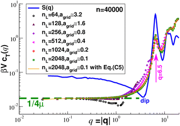 |
| | Fig. 6 Rescaled transverse ICF βVcT(q) for different grid constants agrid as indicated. The open symbols have been obtained using eqn (C4), the thin solid line using eqn (C5) and nL = 2048. Importantly, we obtain the same results in all cases where qurms ≪ 1 and qagrid ≪ 1. Even a rather coarse grid, say for nL = 64, is sufficient to confirm the expected large-wavelength limit (horizontal dashed line). The total static structure factor S(q) is shown for comparison (solid line). The “dip” of S(q) around q ≈ 4 is caused by the polydispersity of the particles as emphasized elsewhere.48S(q) and βVcT(q), at least for sufficiently small agrid, have both a strong peak located similarly at q ≈ 6.5 (arrow). | |
5. Displacement fields
As in previous experimental and numerical studies10,11,21 the displacement field u(r) is constructed from the instantaneous spatial positions ra of the particles a with respect to their reference positions ra. As reference position ra we have used either the average particle position determined using a long trajectory or the particle position after a rapid quench to T = 0. Having not observed any significant quantitative difference between both methods we only report here data computed using the first one. We thus get first the displacement vector ua = ra − ra for each a. By construction the average displacement vector 〈ua〉 must vanish. We find| | | urms ≡ 〈ua2〉 > 1/2 ≈ 0.13 | (C3) |
for the root-mean-squared average urms (sampled over all particles, frames and configurations). The instantaneous displacement field may then be defined by10,11,21| |  | (C4) |
assuming for the moment an infinitessimal fine grid, i.e. agrid → 0. (Different prefactors have been used in ref. 10, 11 and 21). We remind that the δ(r)-function has the dimension “1/volume”. By definition u(r) has thus the same dimension “length” as the displacement vector ua. Following the common definition of the particle flux density,34 the reference position ![[r with combining tilde]](https://www.rsc.org/images/entities/b_char_0072_0303.gif) a in the δ-function may be replaced by the time-dependent position ra, i.e. the displacement field may alternatively be defined by
a in the δ-function may be replaced by the time-dependent position ra, i.e. the displacement field may alternatively be defined by| |  | (C5) |
Both operational definitions are compared for the transverse ICF βVcT(q) in Fig. 6 where data obtained using eqn (C4) are indicated by open symbols. In reciprocal space we obtain| |  | (C6) |
for eqn (C4) and similarly for eqn (C5) with ra replacing ![[r with combining tilde]](https://www.rsc.org/images/entities/b_char_0072_0303.gif) a. Since ra =
a. Since ra = ![[r with combining tilde]](https://www.rsc.org/images/entities/b_char_0072_0303.gif) a+ ua we have to leading order
a+ ua we have to leading order| | | exp(−iq·ra) ≈ exp(−iq·ra)(1 − iq·ua…) | (C7) |
for q|u(q)| ≪ 1. Both operational definitions eqn (C4) and (C5) thus become equivalent for qurms ≪ 1. Due to the small typical (root-mean-squared) displacement urms, eqn (C3), this holds for all sampled q as may be seen from the data presented in Fig. 6. Due to the center-of-mass convention for all particle displacements the volume integral over u(r) must vanish and, equivalently, we have u(q = 0) = 0 in reciprocal space for each instantaneous field. We also remind that the two coordinates of the displacement field in NRC are the longitudinal component uL(q) ≡ u1°(q) and the transverse component uT(q) ≡ u2°(q).
In numerical practice, the continuous field vector r of eqn (C4) and (C5) corresponds to the discrete point on the grid, eqn (B12), closest (using the minimal image convention) to, respectively, the reference position ra or the particle position ra. Strictly speaking, we thus obtain by means of eqn (B10) the FT with respect to their respective closest grid points. (In principle one could directly without approximation compute the displacement field u(q) using eqn (C6) in reciprocal space. Unfortunately, this leads to an additional loop over all n particles for each wavevector q.) The differences between these definitions become neglible for qagrid ≪ 1. That this holds can be clearly seen from Fig. 6 where we have varied agrid over more than one order of magnitude.
6. Linear strain fields
Using the displacement field u(r) the linear (“small”) strain tensor field is defined by8,9| |  | (C8) |
Due to eqn (B3) this becomes| |  | (C9) |
in reciprocal space as already stated in Section IIIB. (Obviously, εαβ = εβα for any r in real space and any q in reciprocal space.) Note that both εαβ(r) and its FT εαβ(q), cf.eqn (B1), are dimensionless fields. Due to our definitions and conventions the macroscopic strain εαβ(q = 0) is assumed to vanish. Using eqn (B12) we numerically determine the relevant components of the (symmetric) strain tensor field εαβ(q) from the two components of the displacement field uα(q) stored on the reciprocal space grid (cf.Fig. 2) and the wavevector qα according to eqn (B12). As noted in Section IIIB, in NRC there are only two non-vanishing strain fields, namely the longitudinal and transverse strain fields εL(q) and εT(q) linearly related to the corresponding displacement fields uL(q) and uT(q), cf.eqn (16) and (17).
7 Correlation function fields
Using the strain tensor fields εαβ(q) in reciprocal space computed according to eqn (C9) for each c and t we obtain the correlation functions cαβγδ(q) = 〈εαβ(q)εγδ(−q)〉 averaged over all c and t. For the reported correlation functions  in a coordinate system turned by an angle α we first compute the new components
  and
and  of displacement field and wavevector. (Alternatively, one may also rotate εγδ(q).) For the ICFs cL(q) and cT(q) obtained using NRC we first get the longitudinal and transverse displacement fields uL(q) and uT(q) in NRC and from those using eqn (16) and (17) the longitudinal and transverse strains εL(q) and εT(q). cL(q) = 〈εL(q)εL(−q)〉 and cT(q) = 〈εT(q)εT(−q)〉 are computed by averaging over all c and t and all wavevectors q with magnitude |q| within a chosen bin around q. The correlation functions cαβγδ(r) in real space (either for unrotated or α-rotated coordinate systems) are finally obtained by inverse FFT.
Appendix D: From cL(q) and cT(q) to cαβγδ(r)
As shown in Appendix A4, a forth-order tensor field describing an isotropic achiral system in two dimensions is given by eqn (A17) in terms of four invariants in(q). In turn these invariants are expressed in terms of the alternative set of invariants cL(q), cT(q), cN(q) and cT(q). Due to eqn (18) we have cN(q) = c⊥(q) = 0 for strain correlations. The correlation function cαβγδ(q) in reciprocal space are thus given by the invariants| |  | (D1) |
and| | | i4(q) =cL(q) − 4cT(q). | (D2) |
More specifically, this implies| | 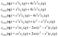 | (D3) |
with c = cos(θ) = ![[q with combining circumflex]](https://www.rsc.org/images/entities/i_char_0071_0302.gif) 1 and s = sin(θ) =
1 and s = sin(θ) = ![[q with combining circumflex]](https://www.rsc.org/images/entities/i_char_0071_0302.gif) 2 being coefficients depending only on the wavevector angle θ. Alternatively, the six relations eqn (D3) may also be obtained using that the components εαβ(q) in the original coordinate frame can be expressed as
2 being coefficients depending only on the wavevector angle θ. Alternatively, the six relations eqn (D3) may also be obtained using that the components εαβ(q) in the original coordinate frame can be expressed as| |  | (D4) |
| |  | (D5) |
| |  | (D6) |
in terms of the longitudinal and transverse strains εL(q) and εT(q) and the fact that εL(q) and εT(q) fluctuate independently. For the correlation functions  in rotated coordinate systems one simply replaces θ by x = θ − α. Note also that
  and
and  do in general not vanish for all x in standard (unrotated or rotated) coordinates. The values for NRC are obtained by setting x = 0, i.e. s = 0 and c = 1. We expand the angle-dependent coefficients before cL(q) and cT(q) in terms of the planar harmonic functions cos(pθ) and sin(pθ) with p being integers using standard trigonometric relations.56 This implies for example
where we have omitted the arguments q on the l.h.s. and q on the r.h.s. The prefactor of cos(4θ) and sin(4θ) is always proportional to i4(q). Having in mind the equipartition relation eqn (2) and using the creep compliances J1 and J2 introduced in eqn (19) one sees that| |  | (D7) |
| |  | (D8) |
in the low- q limit. We thus get in reciprocal space
where the dots mark constant terms. These terms are irrelevant for the inverse FT, only leading to contributions at r = 0. We may thus take advantage of the analytical result for the inverse FT eqn (B18). This leads to| |  | (D9) |
| |  | (D10) |
| |  | (D11) |
| |  | (D12) |
with θ denoting the polar angle of the field vector r. The correlation functions  in rotated coordinate systems generalize the above equations by substituting θ with the angle difference x = θ − α. These results can be rewritten compactly using the general form expected from eqn (A21) for a manifest two-dimensional, isotropic and achiral forth-order tensor field in real space yielding
| | 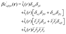 | (D13) |
where the invariants ĩn(r) in real space are given by| | 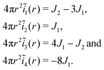 | (D14) |
Since i1 = −(2J1 + J2)/4, i2 = (2J1 + J2)/8, i3 = (2J1 + J2)/4 and i4 = −J1, this is consistent with the more general relation eqn (A22).
The angle dependence for the shear-strain autocorrelation function in real space is investigated in Fig. 7 where we plot using linear coordinates  as a function of x for different r and α. (To obtain sufficiently high statistics we need to average over the indicated finite r-bins. This is done by weighting each data entry for a bin with the proper factor 4πr2.) The data compare well with the prediction, eqn (D9), confirming thus especially the scaling with angle difference x = θ − α. Naturally, the statistics deteriorates with increasing r due to the faster decay of the correlations as compared to the noise.
 |
| | Fig. 7 Rescaled shear-strain autocorrelation function  in real space as a function of x = θ − α comparing data for different r-intervals and rotation angles α with the prediction (bold solid line). in real space as a function of x = θ − α comparing data for different r-intervals and rotation angles α with the prediction (bold solid line). | |
Acknowledgements
We are indebted to the University of Strasbourg for computational resources.
References
-
A. J. McConnell, Applications of Tensor Analysis, Hassell Street Press, 2021 Search PubMed.
-
J. A. Schouten, Tensor Analysis for Physicists, Dover Publications, Oxford, 2015 Search PubMed.
-
W. Schultz-Piszachich, Mathematik 11: Tensoralgebra und -analysis. Thun und Frankfurt/Main, Verlag Harri Deutsch, 1977 Search PubMed.
- J. P. Wittmer, A. N. Semenov and J. Baschnagel, Correlations of tensor field components in isotropic systems with an application to stress correlations in elastic bodies, Phys. Rev. E, 2023, 108, 015002 CrossRef.
-
R. J. A. Lambourne, Relativity, Gravitation, and Cosmology, Cambridge University Press, Cambridge, 2010 Search PubMed.
-
T. Frankel, The Geometry of Physics: An Introduction, Cambridge University Press, Cambridge, 3rd edn, 2012 Search PubMed.
-
P. M. Chaikin and T. C. Lubensky, Principles of condensed matter physics, Cambridge University Press, 1995 Search PubMed.
-
L. D. Landau and E. M. Lifshitz, Theory of Elasticity, Pergamon Press, New York, 1959 Search PubMed.
-
E. B. Tadmor, R. E. Miller and R. S. Elliot, Continuum Mechanics and Thermodynamics, Cambridge University Press, Cambridge, 2012 Search PubMed.
- C. Klix, F. Ebert, F. Weysser, M. Fuchs, G. Maret and P. Keim, Glass elasticity from particle trajectories, Phys. Rev. Lett., 2012, 109, 178301 CrossRef PubMed.
- C. L. Klix, G. Maret and P. Keim, Discontinuous shear modulus determines the glass transition temperature, Phys. Rev. X, 2015, 5, 041033 Search PubMed.
- M. Maier, A. Zippelius and M. Fuchs, Emergence of long-ranged stress correlations at the liquid to glass transition, Phys. Rev. Lett., 2017, 119, 265701 CrossRef PubMed.
- M. Maier, A. Zippelius and M. Fuchs, Stress auto-correlation tensor in glass-forming isothermal fluids: From viscous to elastic response, J. Chem. Phys., 2018, 149, 084502 CrossRef PubMed.
- F. Vogel, A. Zippelius and M. Fuchs, Emergence of Goldstone excitations in stress correlations of glass-forming colloidal dispersions, Europhys. Lett., 2019, 125, 68003 CrossRef CAS.
- A. Lemaître, Tensorial analysis of Eshelby stresses in 3d supercooled liquids, J. Chem. Phys., 2015, 143, 164515 CrossRef.
- A. Lemaître, Stress correlations in glasses, J. Chem. Phys., 2018, 149, 104107 CrossRef PubMed.
- L. Klochko, J. Baschnagel, J. P. Wittmer and A. N. Semenov, Long-range stress correlations in viscoelastic and glass-forming fluids, Soft Matter, 2018, 14, 6835 RSC.
- L. Klochko, J. Baschnagel, J. Wittmer, H. Meyer, O. Benzerara and A. N. Semenov, Theory of length-scale dependent relaxation moduli and stress fluctuations in glass-forming and viscoelastic liquids, J. Chem. Phys., 2022, 156, 164505 CrossRef CAS.
- D. Steffen, L. Schneider, M. Müller and J. Rottler, Molecular simulations and hydrodynamic theory of nonlocal shear stress correlations in supercooled fluids, J. Chem. Phys., 2022, 157, 064501 CrossRef CAS PubMed.
- A. Kabla and G. Debrégeas, Local Stress Relaxation and Shear Banding in a Dry Foam under Shear, Phys. Rev. Lett., 2003, 90, 258303 CrossRef PubMed.
- J. P. Wittmer, H. Xu, O. Benzerara and J. Baschnagel, Fluctuation-dissipation relation between shear stress relaxation modulus and shear stress autocorrelation function revisited, Mol. Phys., 2015, 113, 2881 CrossRef CAS.
- K. W. Desmond and E. R. Weeks, Measurement of Stress Redistribution in Flowing Emulsions, Phys. Rev. Lett., 2015, 115, 098302 CrossRef.
- G. Picard, A. Ajdari, F. Lequeux and L. Bocquet, Elastic consequences of a single plastic event: A step towards the microscopic modeling of the flow of yield stress fluids, Eur. Phys. J. E: Soft Matter Biol. Phys., 2004, 15, 371 CrossRef CAS.
- L. Bocquet, A. Colin and A. Ajdari, Kinetic theory of plastic flow in soft glassy materials, Phys. Rev. Lett., 2009, 103, 036001 CrossRef PubMed.
- J. Chattoraj and A. Lemaître, Elastic Signature of Flow Events in Supercooled Liquids Under Shear, Phys. Rev. Lett., 2013, 111, 066001 CrossRef.
- H. Mizuno, S. Mossa and J. L. Barrat, Measuring spatial distribution of the local elastic modulus in glasses, Phys Rev E, 2013, 87, 042306 CrossRef.
- A. Nicolas, J. Rottler and J. L. Barrat, Spatiotemporal correlations between plastic events in the shear flow of athermal amorphous solids, Eur. Phys. J. E: Soft Matter Biol. Phys., 2014, 37, 50 CrossRef.
- E. Flenner and G. Szamel, Long-range spatial correlations of particle displacements and the emergence of elasticity, Phys. Rev. Lett., 2015, 114, 025501 CrossRef PubMed.
- B. Illing, S. Fritschi, D. Hajnal, C. Klix, P. Keim and M. Fuchs, Strain pattern in supercooled liquids, Phys. Rev. Lett., 2016, 117, 208002 CrossRef PubMed.
- M. Hassani, E. M. Zirdehi, K. Kok, P. Schall, M. Fuchs and F. Varnik, Long-range strain correlations in 3d quiescent glass forming liquids, Europhys. Lett., 2018, 124, 18003 CrossRef.
- C. Liu, G. Biroli, D. R. Reichman and G. Szamel, Dynamics of liquids in the large-dimensional limit, Phys Rev E, 2021, 104, 054606 CrossRef CAS PubMed.
- R. N. Chacko, F. P. Landes, G. Biroli, O. D. A. J. Liu and D. R. Reichman, Elastoplasticity Mediates Dynamical Heterogeneity Below the Mode Coupling Temperature, Phys. Rev. Lett., 2021, 127, 048002 CrossRef CAS PubMed.
-
M. P. Allen and D. J. Tildesley, Computer Simulation of Liquids, Oxford University Press, Oxford, 2nd edon; 2017 Search PubMed.
-
J. P. Hansen and I. R. McDonald, Theory of simple liquids, Academic Press, New York, 3rd edn, 2006 Search PubMed.
-
D. Forster, Hydrodynamic Fluctuations, Broken Symmetry, and Correlation Functions, Perseus Books, New York, 1995 Search PubMed.
- J. P. Wittmer, H. Xu, P. Polińska, F. Weysser and J. Baschnagel, Shear modulus of simulated glass-forming model systems: Effects of boundary condition, temperature and sampling time, J. Chem. Phys., 2013, 138, 12A533 CrossRef CAS PubMed.
- L. Klochko, J. Baschnagel, J. P. Wittmer and A. N. Semenov, Relaxation dynamics in supercooled oligomer liquids: From shear-stress fluctuations to shear modulus and structural correlations, J. Chem. Phys., 2019, 151, 054504 CrossRef.
- G. George, L. Klochko, A. N. Semenov, J. Baschnagel and J. P. Wittmer, Ensemble fluctuations matter for variances of macroscopic variables, Eur. Phys. J. E: Soft Matter Biol. Phys., 2021, 44, 13 CrossRef CAS PubMed.
- G. George, L. Klochko, A. N. Semenov, J. Baschnagel and J. P. Wittmer, Fluctuations of non-ergodic stochastic processes, Eur. Phys. J. E: Soft Matter Biol. Phys., 2021, 44, 54 CrossRef CAS PubMed.
-
J. D. Ferry, Viscoelastic properties of polymers, John Wiley & Sons, New York, 1980 Search PubMed.
-
M. Rubinstein and R. H. Colby, Polymer Physics, Oxford University Press, Oxford, 2003 Search PubMed.
-
M. Doi and S. F. Edwards, The Theory of Polymer Dynamics, Clarendon Press, Oxford, 1986 Search PubMed.
-
J. K. G. Donth, The Glass Transition: Relaxation dynamics in liquids and disordered materials, Springer, Berlin-Heidelberg, 2001 Search PubMed.
- A. Argon and H. Kuo, Plastic flow in a disordered bubble raft (an analog of a metallic glass), Mater. Sci. Eng., 1979, 39, 101 CrossRef.
- D. Rodney, A. Tanguy and D. Vandembroucq, Modeling the mechanics of amorphous solids at different length scale and time scale, Modell. Simul. Mater. Sci. Eng., 2011, 19, 083001 CrossRef.
- A. Nicolas, E. Ferrero, K. Martens and J. L. Barrat, Deformation and flow of amorphous solids: Insights from elastoplastic models, Rev. Mod. Phys., 2018, 90, 045006 CrossRef CAS.
- M. L. Falk and J. S. Langer, Dynamics
of viscoplastic deformation in amorphous solids, Phys Rev E, 1998, 57, 7192 CrossRef CAS.
- L. Klochko, J. Baschnagel, J. P. Wittmer and A. N. Semenov, Relaxation moduli of glass-forming systems: temperature effects and fluctuations, Soft Matter, 2021, 17, 7867 RSC.
- A. Ninarello and L. Berthier, Coslovich D. Models and Algorithms for the Next Generation of Glass Transition Studies, Phys. Rev. X, 2017, 7, 021039 Search PubMed.
-
J. P. Wittmer, A. N. Semenov and J. Baschnagel Strain fluctuations at finite wavevectors for isotropic colloidal glasses using natural rotated coordinates. in preparation. 2023.
- J. P. Vest, G. Tarjus and P. Viot, Mode-coupling approach for the slow dynamics of a liquid on a spherical substrate, J. Chem. Phys., 2015, 143, 084505 CrossRef.
- F. Turci, G. Tarjus and C. P. Royall, From Glass Formation to Icosahedral Ordering by Curving Three-Dimensional Space, Phys. Rev. Lett., 2017, 118, 215501 CrossRef PubMed.
- H. Mizuno and S. Mossa, Mat Phys., 2019, 22, 43604 CAS.
- J. P. Wittmer, A. N. Semenov and J. Baschnagel, Different spatial correlation functions for non-ergodic stochastic processes of macroscopic systems, Eur. Phys. J. E: Soft Matter Biol. Phys., 2022, 45, 65 CrossRef CAS PubMed.
-
W. H. Press, S. A. Teukolsky, W. T. Vetterling and B. P. Flannery, Numerical Recipes in FORTRAN: the art of scientific computing, Cambridge University Press, Cambridge, 1992 Search PubMed.
-
M. Abramowitz and I. A. Stegun, Handbook of Mathematical Functions, Dover, New York, 1964 Search PubMed.
- J. P. Wittmer, H. Xu, P. Polińska, C. Gillig, J. Helfferich and F. Weysser,
et al., Compressibility and pressure correlations in isotropic solids and fluids, Eur. Phys. J. E: Soft Matter Biol. Phys., 2013, 36, 131 CrossRef CAS PubMed.
- J. P. Wittmer, H. Xu and J. Baschnagel, Shear-stress relaxation and ensemble transformation of shear-stress auto-correlation functions revisited, Phys Rev E, 2015, 91, 022107 CrossRef CAS.
- J. F. Lutsko, Stress and elastic constants in anisotropic solids: Molecular dynamics techniques, J. Appl. Phys., 1988, 64, 1152 CrossRef.
- J. F. Lutsko, Generalized expressions for the calculation of elastic constants by computer simulation, J. Appl. Phys., 1989, 65, 2991 CrossRef.
Footnotes |
| † See, e.g., the wikipedia entries on quadrupoles and general multipolar expansions as used, say, in electrostatics. For the planar harmonic basis functions cos(pθ) or sin(pθ) a monopole corresponds to p = 0, a dipole to p = 1, a quadrupole to p = 2 and an octupole to p = 4. |
‡ Let us impose in a rotated coordinate system at α = −π/4 a symmetric source tensor with a finite “shear”  and vanishing diagonal components and vanishing diagonal components  . Using eqn (A2) this implies S11 = −S22 = s and S12 = 0 in the original coordinate system at α = 0. . Using eqn (A2) this implies S11 = −S22 = s and S12 = 0 in the original coordinate system at α = 0. |
§ The omitted constant terms correspond to localized δ(r) contributions to strain correlation functions in real space. For example, such a contribution to c1212(r) is  . . |
¶ The elastic modulus tensor Eαβλδ(q) for isotropic bodies at finite wavevector q is not only characterized by the longitudinal modulus L(q) and the shear modulus G(q) but also by a third modulus M(q) called the “mixed modulus”.17 Note that  , ,  and and  for isotropic bodies in NRC. It is not possible to determine M(q) solely using strain fluctuations. This requires the additional measurement of stress fields in NRC. M(q) may then be obtained using either the appropriate stress–strain or stress–stress correlation functions in reciprocal space.17,50 for isotropic bodies in NRC. It is not possible to determine M(q) solely using strain fluctuations. This requires the additional measurement of stress fields in NRC. M(q) may then be obtained using either the appropriate stress–strain or stress–stress correlation functions in reciprocal space.17,50 |
|| The infinite integral eqn (11.4.16) of ref. 56 is expressed in terms of two coefficients μ and ν which in our case take the (real) values μ = 1 and ν = p. It is stated that eqn (11.4.16) holds for  , being consistent with the condition p > −2 noted in eqn (B17), but also that , being consistent with the condition p > −2 noted in eqn (B17), but also that  , being at first sight in conflict with μ = 1. However, the integral divergence for t → ∞ for μ > 1/2 is fictitious as, e.g., discussed in the Wikipedia entry on “Oscillatory integrals” where it is noted that “Oscillatory integrals make rigorous many arguments that, on a naive level, appear to use divergent integrals”. Note that eqn. (B18) also holds for p = 0 and finite r > 0 which follows from the fact that the FT of a constant is zero everywhere except at the origin. See ref. 4 for an alternative more straight-forward but also more lengthy derivation of eqn. (B18) using the asymptotic behavior of the confluent hypergeometric Kummer function M(a, b, z). , being at first sight in conflict with μ = 1. However, the integral divergence for t → ∞ for μ > 1/2 is fictitious as, e.g., discussed in the Wikipedia entry on “Oscillatory integrals” where it is noted that “Oscillatory integrals make rigorous many arguments that, on a naive level, appear to use divergent integrals”. Note that eqn. (B18) also holds for p = 0 and finite r > 0 which follows from the fact that the FT of a constant is zero everywhere except at the origin. See ref. 4 for an alternative more straight-forward but also more lengthy derivation of eqn. (B18) using the asymptotic behavior of the confluent hypergeometric Kummer function M(a, b, z). |
|
| This journal is © The Royal Society of Chemistry 2023 |
Click here to see how this site uses Cookies. View our privacy policy here.  Open Access Article
 *,
A. N.
Semenov
 and
J.
Baschnagel

 of the instantaneous strain tensor field εαβ(r) in real space. These may be readily obtained33 from the components of the tensor field
 being the Fourier transformed strain tensor field components. (The average 〈…〉 will be specified below) An example for the autocorrelation function c1212(r) of the shear strain ε12(r) is given in Fig. 1 for the same two-dimensional model system already used in ref. 4 and 18. Interestingly, the correlation function is seen to strongly depend both on the orientation of the field vector r (panel (a)) and on the rotation angle α of the coordinate system (panel (b)). Since the simulated system can be shown to be perfectly isotropic down to a few particle diameters,4,18,36–39 these findings beg for an explanation. Expanding on our recent work on stress correlations,4,17,18 this behavior can be traced back to the fact that correlation functions of tensor fields of isotropic systems must be components of a generic isotropic tensor field (cf. Section IIB). This field is shown below (cf. Section IIID) to be completely described in terms of two ICFs cL(q) and cT(q) in reciprocal space (q = |q| being the magnitude of the wavevector). These ICFs characterize the independent fluctuations of the longitudinal and transverse strain components εL(q) and εT(q). Due to the equipartition theorem of statistical physics cL(q) and cT(q) are given by7,10,11,21


![[q with combining circumflex]](https://www.rsc.org/images/entities/i_char_0071_0302.gif) α of the normalized wavevector
α of the normalized wavevector ![[q with combining circumflex]](https://www.rsc.org/images/entities/b_char_0071_0302.gif) and the Kronecker symbol δαβ. Legitimate correlation functions of isotropic systems may thus depend on
and the Kronecker symbol δαβ. Legitimate correlation functions of isotropic systems may thus depend on ![[q with combining circumflex]](https://www.rsc.org/images/entities/i_char_0071_0302.gif) α and, hence, on the orientation of the wavevector and of the coordinate system. While the isotropy of the system may not be manifested by one correlation function, it is crucial for the structure of the complete set of all correlation functions given by eqn (5). We note finally that it is useful to express the above ICFs in terms of an alternative set of ICFs cL(q), cT(q), c⊥(q) and cN(q) given by
α and, hence, on the orientation of the wavevector and of the coordinate system. While the isotropy of the system may not be manifested by one correlation function, it is crucial for the structure of the complete set of all correlation functions given by eqn (5). We note finally that it is useful to express the above ICFs in terms of an alternative set of ICFs cL(q), cT(q), c⊥(q) and cN(q) given by
![[q with combining circumflex]](https://www.rsc.org/images/entities/i_char_0071_0302.gif) α one may, quite generally, express all isotropic tensor fields in two dimensions in terms of the orthogonal planar harmonic basis functions cos(pθ) and sin(pθ) with
α one may, quite generally, express all isotropic tensor fields in two dimensions in terms of the orthogonal planar harmonic basis functions cos(pθ) and sin(pθ) with ![[q with combining circumflex]](https://www.rsc.org/images/entities/i_char_0071_0302.gif) 1 = cos(θ) and
1 = cos(θ) and ![[q with combining circumflex]](https://www.rsc.org/images/entities/i_char_0071_0302.gif) 2 = sin(θ) and p = 0, 2 and 4. (See Appendix D for more details.) For instance, it follows from eqn (5) that
2 = sin(θ) and p = 0, 2 and 4. (See Appendix D for more details.) For instance, it follows from eqn (5) that
 in real space must have the same mathematical properties.


 . We shall say more about the specific linear strain response in real space in Section V but focus here on the generic response in reciprocal space. Being symmetric the source tensor may be diagonalized by a rotation of the coordinate system where s12 = s21 = 0 and s11 and s22 become the two (in general not identical) eigenvalues. Hence,
![[q with combining circumflex]](https://www.rsc.org/images/entities/i_char_0071_0302.gif) α
α![[q with combining circumflex]](https://www.rsc.org/images/entities/i_char_0071_0302.gif) β
β![[q with combining circumflex]](https://www.rsc.org/images/entities/i_char_0071_0302.gif) 1
1![[q with combining circumflex]](https://www.rsc.org/images/entities/i_char_0071_0302.gif) 2 ∝ sin(2θ)
2 ∝ sin(2θ)![[q with combining circumflex]](https://www.rsc.org/images/entities/i_char_0071_0302.gif) 1
1![[q with combining circumflex]](https://www.rsc.org/images/entities/i_char_0071_0302.gif) 2(
2(![[q with combining circumflex]](https://www.rsc.org/images/entities/i_char_0071_0302.gif) 12 −
12 − ![[q with combining circumflex]](https://www.rsc.org/images/entities/i_char_0071_0302.gif) 22) ∝ sin(4θ).
22) ∝ sin(4θ).![[thin space (1/6-em)]](https://www.rsc.org/images/entities/char_2009.gif) 000 and 40
000 and 40![[thin space (1/6-em)]](https://www.rsc.org/images/entities/char_2009.gif) 000 particles at a working temperature T = 0.2. This is much lower than the glass transition temperature Tg ≈ 0.26,36i.e. for any computationally feasible production time the systems behave as solid elastic bodies.38Nc = 200 completely independent configurations c are prepared using a mix of local and swap MC hopping moves38,49 while the presented data are computed using local MC moves only. For each c we store time-series containing Nt = 10
000 particles at a working temperature T = 0.2. This is much lower than the glass transition temperature Tg ≈ 0.26,36i.e. for any computationally feasible production time the systems behave as solid elastic bodies.38Nc = 200 completely independent configurations c are prepared using a mix of local and swap MC hopping moves38,49 while the presented data are computed using local MC moves only. For each c we store time-series containing Nt = 10![[thin space (1/6-em)]](https://www.rsc.org/images/entities/char_2009.gif) 000 “frames” t computed using equidistant time intervals. As described in Appendix C3, the elastic modulus tensor is isotropic and determined by the two Lamé coefficients λ ≈ 38 and μ ≈ 14.36,38
000 “frames” t computed using equidistant time intervals. As described in Appendix C3, the elastic modulus tensor is isotropic and determined by the two Lamé coefficients λ ≈ 38 and μ ≈ 14.36,38
 the strain tensor field8,17
 are obtained using the components
  and
and  in the rotated frame.
 for all wavevectors q. Using the components
  and
and  we obtain (as before) the strain tensor
  . Importantly,
 ,
,  ,
,  and
and  for the longitudinal and transverse components of the displacement and strain tensor fields. Note that

 may for finite Nc not only depend on q but also on
 ![[q with combining circumflex]](https://www.rsc.org/images/entities/b_char_0071_0302.gif) . Consistently with eqn (A18) and ref. 4, 17 and 18 we thus operationally define the ICFs
. Consistently with eqn (A18) and ref. 4, 17 and 18 we thus operationally define the ICFs  ,
,  ,
,  and
and  by averaging over all wavevectors with |q| ≈ q. However,
  implies immediately that
 and
and  as functions of the wavevector angle θ for one small wavevector with q ≈ 0.1. As expected for isotropic systems, these correlation functions are θ-independent (apart from a small noise contribution due to the finite number of independent configurations). The main panel presents the
 ![[q with combining circumflex]](https://www.rsc.org/images/entities/i_char_0071_0302.gif) -averaged longitudinal and transverse ICFs βVcL(q) and βVcT(q) as functions of q. The expected large-wavelength limit eqn (2) is indicated in both panels by bold horizontal lines. As can be seen in the main panel, it is well confirmed for q ≪ 1 over at least one order of magnitude where we have used the known values of λ and μ. We remind that eqn (2) has been used in various experimental and numerical studies10,11,21 to fit λ and μ. cL(q) and cT(q) characterize the typical length of the complex random variables εL(q) and εT(q). Their distributions and correlations will be discussed elsewhere.50 We note finally that the increase of the ICFs from the low-q asymptotics visible for q > 1 correlates with the deviation of the total static structure factor S(q) from its low-q plateau (cf.Fig. 6).
-averaged longitudinal and transverse ICFs βVcL(q) and βVcT(q) as functions of q. The expected large-wavelength limit eqn (2) is indicated in both panels by bold horizontal lines. As can be seen in the main panel, it is well confirmed for q ≪ 1 over at least one order of magnitude where we have used the known values of λ and μ. We remind that eqn (2) has been used in various experimental and numerical studies10,11,21 to fit λ and μ. cL(q) and cT(q) characterize the typical length of the complex random variables εL(q) and εT(q). Their distributions and correlations will be discussed elsewhere.50 We note finally that the increase of the ICFs from the low-q asymptotics visible for q > 1 correlates with the deviation of the total static structure factor S(q) from its low-q plateau (cf.Fig. 6).

 and
and  vs. θ for q ≈ 0.1. Main panel: Semi-logarithmic representation of ICFs βVcT(q) and βVcL(q) vs. q.


 in rotated coordinate systems one merely needs to substitute θ by x = θ − α. These relations are put to a test in Fig. 4 where we focus for clarity on the reduced shear-strain autocorrelation function
  for n = 40
![[thin space (1/6-em)]](https://www.rsc.org/images/entities/char_2009.gif) 000. The angular dependences are presented in the main panel for one wavevector in the low-q limit. Focusing on the first term in eqn (20) we have taken off the mean constant average over all θ (corresponding to the dots). Importantly, all data for different α are seen to collapse when plotted as a function of the scaling variable x. Obviously, this simple scaling (without characteristic angle) would not hold for anisotropic systems. To obtain a precise test of the q-dependence of cαβγδ(q) we project out the angular dependences using
000. The angular dependences are presented in the main panel for one wavevector in the low-q limit. Focusing on the first term in eqn (20) we have taken off the mean constant average over all θ (corresponding to the dots). Importantly, all data for different α are seen to collapse when plotted as a function of the scaling variable x. Obviously, this simple scaling (without characteristic angle) would not hold for anisotropic systems. To obtain a precise test of the q-dependence of cαβγδ(q) we project out the angular dependences using

 for n = 40
![[thin space (1/6-em)]](https://www.rsc.org/images/entities/char_2009.gif) 000. Main panel: Angle dependence of vertically shifted f(q) for q ≈ 0.1. Data collapse is observed using the reduced angle x = θ−α. The bold solid line indicates the prediction, eqn (20). Inset: Comparison of P[f,p](q) for p = 4 with the predicted low-q limit J1/8 (bold solid line).
000. Main panel: Angle dependence of vertically shifted f(q) for q ≈ 0.1. Data collapse is observed using the reduced angle x = θ−α. The bold solid line indicates the prediction, eqn (20). Inset: Comparison of P[f,p](q) for p = 4 with the predicted low-q limit J1/8 (bold solid line). in real space. As shown in Appendix D, inverse FT implies
 and for
  . Moreover,
![[thin space (1/6-em)]](https://www.rsc.org/images/entities/char_2009.gif) 000 several rescaled correlation functions f(r) are presented in Fig. 5. In agreement with eqn (25) the indicated first three cases collapse for p = 4 and r ≳ 20 on J1/4πr2 (bold solid line). This confirms the octupolar symmetry of these correlation functions. Confirming eqn (26) the last case with f(r) = −β(c1111(r) − c2222(r))/2 collapses onto J2/4πr2 (dashed line). p = 2 is used here in agreement with the predicted quadrupolar symmetry of this correlation function. Similar results are obtained for other particle numbers n.
000 several rescaled correlation functions f(r) are presented in Fig. 5. In agreement with eqn (25) the indicated first three cases collapse for p = 4 and r ≳ 20 on J1/4πr2 (bold solid line). This confirms the octupolar symmetry of these correlation functions. Confirming eqn (26) the last case with f(r) = −β(c1111(r) − c2222(r))/2 collapses onto J2/4πr2 (dashed line). p = 2 is used here in agreement with the predicted quadrupolar symmetry of this correlation function. Similar results are obtained for other particle numbers n.
![[small epsilon, Greek, circumflex]](https://www.rsc.org/images/entities/i_char_e107.gif) αβ(r) = εαβ(r, t). Extending very briefly our discussion to the time domain, let us introduce the time-dependent correlation functions
αβ(r) = εαβ(r, t). Extending very briefly our discussion to the time domain, let us introduce the time-dependent correlation functions
 of the system with δσαβ(r) being an imposed external stress field. This is equivalent to the application of an appropriate external perturbative force field to each particle. For a general “growth function”42 in response to a sudden application of a step field, such as eqn (28), the relevant FDT relations are stated (for scalar fields) by eqn (3.65) and (3.67) of ref. 42. The mean strain increment δεαβ(r, t) induced by this perturbation is then given in real space by a convolution integral for the time-dependent correlation functions cαβγδ(r, t) and the stress perturbation δσαβ(r). Using eqn (B6) this relation may be written more compactly in reciprocal space as
 at switched off external perturbation
  ) must, of course, vanish
 denoting the long-time creep and
  standing for the spatial correlation function without time lag, eqn (1), as everywhere else in this paper.
![[r with combining circumflex]](https://www.rsc.org/images/entities/i_char_0072_0302.gif) αsαβ
αsαβ![[r with combining circumflex]](https://www.rsc.org/images/entities/i_char_0072_0302.gif) β/2 this may be written quite generally
β/2 this may be written quite generally

![[r with combining circumflex]](https://www.rsc.org/images/entities/i_char_0072_0302.gif) 12 −
12 − ![[r with combining circumflex]](https://www.rsc.org/images/entities/i_char_0072_0302.gif) 22)/2. Using eqn (13) or eqn (35) this yields
22)/2. Using eqn (13) or eqn (35) this yields

![[thin space (1/6-em)]](https://www.rsc.org/images/entities/char_2009.gif) 17,48,50 It can be shown50 that both the isotropicity and the harmonicity of the strain modes assumed in the derivation of eqn (38) are well justified for the present model up to q ≈ 1 while deviations become relevant for larger wavevectors, especially around the main peak of the static structure factor S(q).
17,48,50 It can be shown50 that both the isotropicity and the harmonicity of the strain modes assumed in the derivation of eqn (38) are well justified for the present model up to q ≈ 1 while deviations become relevant for larger wavevectors, especially around the main peak of the static structure factor S(q).

 denoting the FT as discussed in Appendix B).
 with matrix coefficients cαβ given by the direction cosine
  .3 We remind that3

 remains unchanged by these “passive” transforms albeit its coordinates change.


 which reduces to eqn (A4) for q = 0. Please note that the fields on the left handside of eqn (A6) are evaluated with the original coordinates of the vector field variable q while the fields on the right handside are evaluated with the transformed coordinates. Another way to state this is to say that the left hand fields are computed at the original vector q = (q1,…,qd) while the right hand fields are computed at the “actively transformed” vector
  . It is for this reason that finite components with an odd number of equal indices, e.g., T1222(q) ≠ 0, are possible in principle for finite q.
 with q = |q|. These tensor field components in NRC are marked by “°” to distinguish them from standard rotated tensor fields (marked by primes “′”) where the same rotation is used for all q. If in addition
  is an even function of its field variable q (as in the case of achiral systems for even order o) it can be shown4 that all tensor field components with an odd number of equal indices must vanish.

 , cf.eqn (14), or the source tensor sαβ needed for a response field, cf.eqn (8). We assume for all forth-order tensor fields that
![[T with combining circumflex]](https://www.rsc.org/images/entities/i_char_0054_0302.gif) αβ(q)
αβ(q)![[T with combining circumflex]](https://www.rsc.org/images/entities/i_char_0054_0302.gif) γδ(−q)〉 with
γδ(−q)〉 with ![[T with combining circumflex]](https://www.rsc.org/images/entities/i_char_0054_0302.gif) αβ(q) being an instantaneous second-order tensor field. eqn (A8) then follows from the symmetry of the second-order tensor fields. The evenness of forth-order tensor fields, eqn (A10), is a necessary condition for achiral systems. It implies that Tαβγδ(q) is real if Tαβγδ(r) is real and, moreover, eqn (A9) for correlation functions since
αβ(q) being an instantaneous second-order tensor field. eqn (A8) then follows from the symmetry of the second-order tensor fields. The evenness of forth-order tensor fields, eqn (A10), is a necessary condition for achiral systems. It implies that Tαβγδ(q) is real if Tαβγδ(r) is real and, moreover, eqn (A9) for correlation functions since![[T with combining circumflex]](https://www.rsc.org/images/entities/i_char_0054_0302.gif) αβ(q)
αβ(q)![[T with combining circumflex]](https://www.rsc.org/images/entities/i_char_0054_0302.gif) γδ(−q)〉 = 〈
γδ(−q)〉 = 〈![[T with combining circumflex]](https://www.rsc.org/images/entities/i_char_0054_0302.gif) γδ(q)
γδ(q)![[T with combining circumflex]](https://www.rsc.org/images/entities/i_char_0054_0302.gif) αβ(−q)〉.
αβ(−q)〉.![[q with combining circumflex]](https://www.rsc.org/images/entities/i_char_0071_0302.gif) α
α![[q with combining circumflex]](https://www.rsc.org/images/entities/i_char_0071_0302.gif) α
α![[q with combining circumflex]](https://www.rsc.org/images/entities/i_char_0071_0302.gif) β
β![[q with combining circumflex]](https://www.rsc.org/images/entities/i_char_0071_0302.gif) αδβγ + j2(q)
αδβγ + j2(q)![[q with combining circumflex]](https://www.rsc.org/images/entities/i_char_0071_0302.gif) βδαγ + j3(q)
βδαγ + j3(q)![[q with combining circumflex]](https://www.rsc.org/images/entities/i_char_0071_0302.gif) γδαβ + j4(q)
γδαβ + j4(q)![[q with combining circumflex]](https://www.rsc.org/images/entities/i_char_0071_0302.gif) α
α![[q with combining circumflex]](https://www.rsc.org/images/entities/i_char_0071_0302.gif) β
β![[q with combining circumflex]](https://www.rsc.org/images/entities/i_char_0071_0302.gif) γ
γ
![[q with combining circumflex]](https://www.rsc.org/images/entities/i_char_0071_0302.gif) α of the normalized wavevector
α of the normalized wavevector ![[q with combining circumflex]](https://www.rsc.org/images/entities/b_char_0071_0302.gif) and thus on the orientations of the field vector and of the coordinate system.
and thus on the orientations of the field vector and of the coordinate system.

![[q with combining circumflex]](https://www.rsc.org/images/entities/b_char_0071_0302.gif) of the wavevector q. Importantly, all other components
of the wavevector q. Importantly, all other components  are either by eqn (A8) and (A9) identical to these invariants or must vanish for an odd number of equal indices as reminded in Section A2. The d4 = 16 components
  are thus completely determined by the four invariants and this for any q. Tαβγδ(q) is then obtained by the inverse rotation to the original unrotated frame using eqn (A2). It is readily seen that
![[k with combining tilde]](https://www.rsc.org/images/entities/i_char_006b_0303.gif) 1(r)δαβ +
1(r)δαβ + ![[k with combining tilde]](https://www.rsc.org/images/entities/i_char_006b_0303.gif) 2(r)
2(r)![[r with combining circumflex]](https://www.rsc.org/images/entities/i_char_0072_0302.gif) α
α![[r with combining circumflex]](https://www.rsc.org/images/entities/i_char_0072_0302.gif) β
β
![[k with combining tilde]](https://www.rsc.org/images/entities/i_char_006b_0303.gif) n(r) and ĩn(r) denoting the invariants in real space and
n(r) and ĩn(r) denoting the invariants in real space and ![[r with combining circumflex]](https://www.rsc.org/images/entities/i_char_0072_0302.gif) α = rα/r components of the normalized vector
α = rα/r components of the normalized vector ![[r with combining circumflex]](https://www.rsc.org/images/entities/b_char_0072_0302.gif) = r/r. As already stated, eqn (A1), the tensor field components in real and reciprocal space are related by FT. Note that
= r/r. As already stated, eqn (A1), the tensor field components in real and reciprocal space are related by FT. Note that ![[k with combining tilde]](https://www.rsc.org/images/entities/i_char_006b_0303.gif) n(r) and ĩn(r) are in general not the FTs of, respectively, kn(q) and in(q). For the important case that the invariants in reciprocal space are q-independent constants it follows quite generally that
n(r) and ĩn(r) are in general not the FTs of, respectively, kn(q) and in(q). For the important case that the invariants in reciprocal space are q-independent constants it follows quite generally that
 from “real space” (variable r) to “reciprocal space” (variable q) is defined by


 and
and  this implies according to the “convolution theorem”55


 and
and  being discrete sums over nV = ndL = V/adgrid grid points in, respectively, real or reciprocal space. As shown in Fig. 2 we label the grid points in real and reciprocal space using

![[r with combining circumflex]](https://www.rsc.org/images/entities/char_0072_0302.gif) = (cos(θr), sin(θr)). We make now the substitution θ = θq − θr and use that56
= (cos(θr), sin(θr)). We make now the substitution θ = θq − θr and use that56


 . As may be seen from eqn (11.4.16) of ref. 56 the latter integral becomes||

![[thin space (1/6-em)]](https://www.rsc.org/images/entities/char_2009.gif) 000 particles. We first equilibrate = 200 independent configurations c at a high temperature T = 0.55 in the liquid limit. These configurations are adiabatically cooled down using a combination of local MC moves33 and swap MC moves exchanging the sizes of pairs of particles.38,49 In addition, an MC barostat33 imposes an average normal stress P = 2.36,38 At the working temperature T = 0.2 we first thoroughly temper over Δτ = 107 all configurations with switched-on local, swap and barostat MC moves and then again over Δτ = 107 with switched-on local and swap moves and switched-off barostat moves. The final production runs are carried out at constant volume V only keeping local MC moves. Under these conditions, T = 0.2 is well below the glass transition temperature Tg ≈ 0.26 determined in previous work.36,38 Due to the barostat used for the cooling the box volume V = Ld differs slightly between different configurations c while V is identical for all frames t of the time-series of the same configuration c. In all cases the number density is of order unity. For each particle number n and each of the independent configurations c we store ensembles of time series containing = 10
000 particles. We first equilibrate = 200 independent configurations c at a high temperature T = 0.55 in the liquid limit. These configurations are adiabatically cooled down using a combination of local MC moves33 and swap MC moves exchanging the sizes of pairs of particles.38,49 In addition, an MC barostat33 imposes an average normal stress P = 2.36,38 At the working temperature T = 0.2 we first thoroughly temper over Δτ = 107 all configurations with switched-on local, swap and barostat MC moves and then again over Δτ = 107 with switched-on local and swap moves and switched-off barostat moves. The final production runs are carried out at constant volume V only keeping local MC moves. Under these conditions, T = 0.2 is well below the glass transition temperature Tg ≈ 0.26 determined in previous work.36,38 Due to the barostat used for the cooling the box volume V = Ld differs slightly between different configurations c while V is identical for all frames t of the time-series of the same configuration c. In all cases the number density is of order unity. For each particle number n and each of the independent configurations c we store ensembles of time series containing = 10![[thin space (1/6-em)]](https://www.rsc.org/images/entities/char_2009.gif) 000 instantaneous “frames” t. These are obtained using the equidistant time intervals δτ = 1000 for n = 10
000 instantaneous “frames” t. These are obtained using the equidistant time intervals δτ = 1000 for n = 10![[thin space (1/6-em)]](https://www.rsc.org/images/entities/char_2009.gif) 000 and δτ = 100 for the other system sizes.
000 and δτ = 100 for the other system sizes.


![[r with combining tilde]](https://www.rsc.org/images/entities/b_char_0072_0303.gif) a in the δ-function may be replaced by the time-dependent position ra, i.e. the displacement field may alternatively be defined by
a in the δ-function may be replaced by the time-dependent position ra, i.e. the displacement field may alternatively be defined by

![[r with combining tilde]](https://www.rsc.org/images/entities/b_char_0072_0303.gif) a. Since ra =
a. Since ra = ![[r with combining tilde]](https://www.rsc.org/images/entities/b_char_0072_0303.gif) a+ ua we have to leading order
a+ ua we have to leading order

 in a coordinate system turned by an angle α we first compute the new components
  and
and  of displacement field and wavevector. (Alternatively, one may also rotate εγδ(q).) For the ICFs cL(q) and cT(q) obtained using NRC we first get the longitudinal and transverse displacement fields uL(q) and uT(q) in NRC and from those using eqn (16) and (17) the longitudinal and transverse strains εL(q) and εT(q). cL(q) = 〈εL(q)εL(−q)〉 and cT(q) = 〈εT(q)εT(−q)〉 are computed by averaging over all c and t and all wavevectors q with magnitude |q| within a chosen bin around q. The correlation functions cαβγδ(r) in real space (either for unrotated or α-rotated coordinate systems) are finally obtained by inverse FFT.


![[q with combining circumflex]](https://www.rsc.org/images/entities/i_char_0071_0302.gif) 1 and s = sin(θ) =
1 and s = sin(θ) = ![[q with combining circumflex]](https://www.rsc.org/images/entities/i_char_0071_0302.gif) 2 being coefficients depending only on the wavevector angle θ. Alternatively, the six relations eqn (D3) may also be obtained using that the components εαβ(q) in the original coordinate frame can be expressed as
2 being coefficients depending only on the wavevector angle θ. Alternatively, the six relations eqn (D3) may also be obtained using that the components εαβ(q) in the original coordinate frame can be expressed as


 in rotated coordinate systems one simply replaces θ by x = θ − α. Note also that
  and
and  do in general not vanish for all x in standard (unrotated or rotated) coordinates. The values for NRC are obtained by setting x = 0, i.e. s = 0 and c = 1. We expand the angle-dependent coefficients before cL(q) and cT(q) in terms of the planar harmonic functions cos(pθ) and sin(pθ) with p being integers using standard trigonometric relations.56 This implies for example


 in rotated coordinate systems generalize the above equations by substituting θ with the angle difference x = θ − α. These results can be rewritten compactly using the general form expected from eqn (A21) for a manifest two-dimensional, isotropic and achiral forth-order tensor field in real space yielding

 as a function of x for different r and α. (To obtain sufficiently high statistics we need to average over the indicated finite r-bins. This is done by weighting each data entry for a bin with the proper factor 4πr2.) The data compare well with the prediction, eqn (D9), confirming thus especially the scaling with angle difference x = θ − α. Naturally, the statistics deteriorates with increasing r due to the faster decay of the correlations as compared to the noise.
 in real space as a function of x = θ − α comparing data for different r-intervals and rotation angles α with the prediction (bold solid line).
 and vanishing diagonal components
  . Using eqn (A2) this implies S11 = −S22 = s and S12 = 0 in the original coordinate system at α = 0.
 .
. ,
,  and
and  for isotropic bodies in NRC. It is not possible to determine M(q) solely using strain fluctuations. This requires the additional measurement of stress fields in NRC. M(q) may then be obtained using either the appropriate stress–strain or stress–stress correlation functions in reciprocal space.17,50
 , being consistent with the condition p > −2 noted in eqn (B17), but also that
  , being at first sight in conflict with μ = 1. However, the integral divergence for t → ∞ for μ > 1/2 is fictitious as, e.g., discussed in the Wikipedia entry on “Oscillatory integrals” where it is noted that “Oscillatory integrals make rigorous many arguments that, on a naive level, appear to use divergent integrals”. Note that eqn. (B18) also holds for p = 0 and finite r > 0 which follows from the fact that the FT of a constant is zero everywhere except at the origin. See ref. 4 for an alternative more straight-forward but also more lengthy derivation of eqn. (B18) using the asymptotic behavior of the confluent hypergeometric Kummer function M(a, b, z).
