
 Open Access Article
 This Open Access Article is licensed under a Creative Commons Attribution-Non Commercial 3.0 Unported Licence
Defying the inverse energy gap law: a vacuum-evaporable Fe(II) low-spin complex with a long-lived LIESST state†
Jan
Grunwald
a,
Jorge
Torres
b,
Axel
Buchholz
 c,
Christian
Näther
a,
Lea
Kämmerer
d,
Manuel
Gruber
d,
Sebastian
Rohlf
e,
Sangeeta
Thakur
b,
Heiko
Wende
d,
Winfried
Plass
c,
Wolfgang
Kuch
*b and
Felix
Tuczek
*a
c,
Christian
Näther
a,
Lea
Kämmerer
d,
Manuel
Gruber
d,
Sebastian
Rohlf
e,
Sangeeta
Thakur
b,
Heiko
Wende
d,
Winfried
Plass
c,
Wolfgang
Kuch
*b and
Felix
Tuczek
*a
aInstitut für Anorganische Chemie, Christian-Albrechts-Universität zu Kiel, 24098 Kiel, Germany. E-mail: ftuczek@ac.uni-kiel.de; Fax: +49 431 880 1520; Tel: +49 431 880 1410
bInstitut für Experimentalphysik, Freie Universität Berlin, Arnimallee 14, 14195 Berlin, Germany. E-mail: wolfgang.kuch@fu-berlin.de; Fax: +49 30 838 452098; Tel: +49 30 838 52098
cInstitut für Anorganische und Analytische Chemie, Friedrich-Schiller-Universität Jena, 07743 Jena, Germany
dFakultät für Physik and CENIDE, Universität Duisburg-Essen, 47048 Duisburg, Germany
eInstitut für Experimentelle und Angewandte Physik, Christian-Albrechts-Universität zu Kiel, 24098 Kiel, Germany
First published on 26th May 2023
Abstract
The novel vacuum-evaporable complex [Fe(pypypyr)2] (pypypyr = bipyridyl pyrrolide) was synthesised and analysed as bulk material and as a thin film. In both cases, the compound is in its low-spin state up to temperatures of at least 510 K. Thus, it is conventionally considered a pure low-spin compound. According to the inverse energy gap law, the half time of the light-induced excited high-spin state of such compounds at temperatures approaching 0 K is expected to be in the regime of micro- or nanoseconds. In contrast to these expectations, the light-induced high-spin state of the title compound has a half time of several hours. We attribute this behaviour to a large structural difference between the two spin states along with four distinct distortion coordinates associated with the spin transition. This leads to a breakdown of single-mode behaviour and thus drastically decreases the relaxation rate of the metastable high-spin state. These unprecedented properties open up new strategies for the development of compounds showing light-induced excited spin state trapping (LIESST) at high temperatures, potentially around room temperature, which is relevant for applications in molecular spintronics, sensors, displays and the like.
1 Introduction
The introduction of function on a molecular level as opposed to bulk material has gained increased interest in recent years.1–3 Aside from completely new applications, functional molecules bear the potential for miniaturisation of current devices. In particular, so-called spin-crossover (SCO) complexes that can be switched between two states with distinct optical, magnetic, geometric and electronic properties4–13 are attractive for the development of sensors,14–19 actuators,20,21 displays22,23 and data storage.22,24–29 Spin-crossover is most often found in octahedral complexes with Fe(II) as the central atom, but can generally occur in transition metal complexes with two different electronic ground states.30–36 For octahedral complexes this is possible with electron configurations of d4–d7. One possible arrangement of the electrons is according to maximum spin, following Hund's rule (see Fig. 1a). This arrangement is called the high-spin state (HS). On the other hand, the low-spin state (LS) describes the arrangement where energetically favoured orbitals are occupied first, leading to minimum spin. If those two states are close enough in energy, external stimuli such as temperature, pressure or light can induce a spin transition that is called spin-crossover. Thermally induced SCO is characterised by the temperature T1/2 at which equal fractions of molecules are in the two spin states. The steepness of thermal SCO is strongly influenced by intermolecular interactions. These cooperative effects occur predominantly in bulk material and can result in abrupt, incomplete or step-wise transitions, as well as hystereses.31 Light-induced spin transition is of interest for a broad range of applications. Here, in the case of metal centres with an electron configuration of d6 (e.g., Fe(II)), excitation of d–d or charge-transfer transitions from the ground state (LS) via light followed by two intersystem-crossing steps leads to the metastable HS state.30,31,37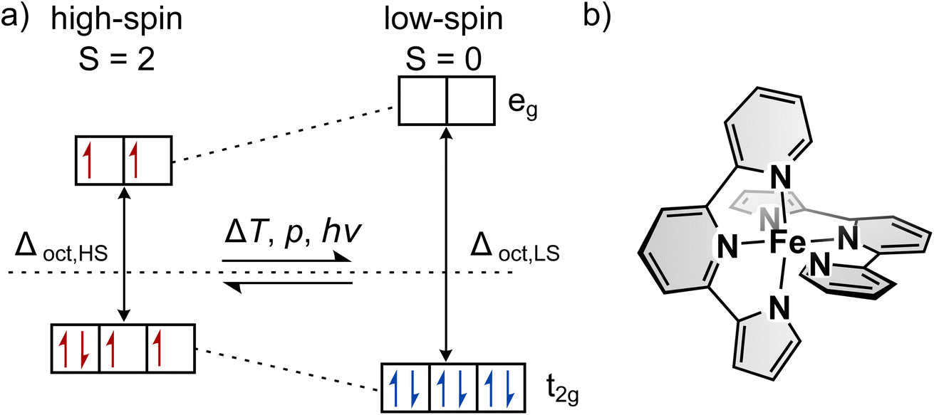 | ||
| Fig. 1 (a) Octahedral ligand field splitting and electron occupation for a central atom with an electron configuration of d6, such as Fe(II). The high-spin state with maximum spin (S = 2, left) and the low-spin state with minimum spin (S = 0, right) are shown. (b) Structure of the synthesised and investigated complex [Fe(pypypyr)2]. | ||
While light-induced spin transition occurs at all temperatures, the lifetime of the metastable HS state drastically depends on the temperature: only at low temperatures (typically below 100 K) is the thermal relaxation rate low enough to effectively trap the molecules in the metastable state. Hence, this effect is called the light-induced excited spin state trapping (LIESST) effect.31 Due to the desire for light-induced spin-crossover at ambient temperatures, extensive effort has been put into research to increase TLIESST, the temperature at which the metastable state becomes unstable. According to the inverse energy gap law, the nonadiabatic tunneling rate that governs the relaxation process at low temperatures increases with increasing T1/2.30,33,38 Hence, to the best of our knowledge, no Fe(II) complex with a transition temperature significantly above room temperature (typically referred to as an LS compound) has been found whose LIESST state is stable long enough to be observed with common analytics, without stabilising the HS state in a matrix39,40 or by changing the coordination number.41–45
For many potential applications, it is necessary to deposit the SCO compounds on surfaces as thin films.46–48 While there are several methods to realize this,49,50 such as lithographic methods,51–53 drop casting,54,55 spin coating,56–59 Langmuir–Blodgett techniques60–64 and electrospray ionisation deposition,65–67 physical vapour deposition (PVD) or sublimation has been found to be optimal in practice,46,47,68 as this method does not require any uncommon equipment and works without solvents. However, it requires the compounds to sublime before thermal decomposition. This was first shown successfully for [Fe(phen)2(NCS)2] (phen = 1,10-phenanthroline),68–72 followed by several complexes based on bi-73–80 or tridentate81–90 borate ligands and more recently for two tridentate ligands with one oxygen donor atom.65,91 The only other complexes with a [FeN6] coordination sphere that are not based on borate ligands are [Fe(NCS)2(L)] based on the neutral tetradentate ligand 1-{6-[1,1-di(pyridin-2-yl)ethyl]-pyridin-2-yl}-N,N-dimethylmethanamine92 and [Fe(py(CF3)2pyr)2(phen)] (pypyr = 2-(pyridine-2-yl)pyrrolide).93
A common problem found with SCO molecules on surfaces is their instability in direct contact with noble metals.66,71,94–96 Strategies to increase their stability include a higher chelate effect and anionic ligands. Thus, the two best approaches seem to be either two monoanionic tridentate ligands or one bianionic hexadentate ligand. This hypothesis is supported by the fact that the only two complexes that have been shown to be functional in direct contact with noble metals belong to the former category.97,98 Following this strategy, we synthesised a new complex based on a tridentate version of the above-mentioned pyridyl pyrrolide ligand, i.e., bipyridyl pyrrolide (pypypyr). This ligand was originally designed and synthesised for potential analytical application for luminescence degradation measurements on photocatalytic surfaces.99 Its Co(II) complex was investigated theoretically towards its use as a redox mediator.100 However, to the best of our knowledge, so far this ligand has not been successfully coordinated to any metal ion. Only a Ru(II) complex of a biphenyl substituted variant has been synthesised.101 Thus, in the following, the synthesis and characterisation of the first two transition metal complexes of pypypyr are presented.
2 Results and discussion
2.1 Synthesis
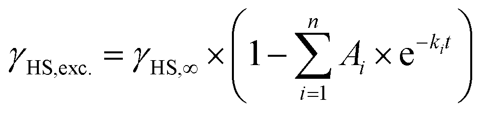
The ligand synthesis of pypypyrH was very straight-forward, following the protocol from Böttger et al.99 with only small alterations (see Fig. 2). Briefly, we synthesised 6-bromo-2,2′-bipyridine using a one-step Negishi coupling reaction instead of the three-step synthesis by Böttger et al. However, the synthesis of the iron(II) complex [Fe(pypypyr)2] proved to be more complicated. After trying several bases to deprotonate the ligand, we found the weakest base with sufficient basicity to be KOtBu in acetonitrile, whereas the same base in tetrahydrofuran was not effective. Afterwards, we tried a vast amount of combinations of iron(II) precursors and solvents to remove the side product (salt consisting of the cation from the base and the anion from the precursor). In our hands, Fe(BF4)·6H2O in acetonitrile and the addition of deoxygenated water leading to near complete precipitation of the target complex gave the best results. While free of any starting materials or side products, the resulting powder was still contaminated by traces of impurities (i.e., solvents with ca. 1 mol%) that we were unable to remove using heat and vacuum. Still, NMR spectroscopy, high-resolution mass spectrometry and crystal structure analysis proved the successful synthesis of [Fe(pypypyr)2], which was investigated using various physicochemical and spectroscopic methods described in the following. | ||
| Fig. 2 Overview of the synthesis of the ligand pypypyrH and its neutral metal complexes. First, 6-bromo-2,2′-bipyridine was synthesised using an in situ Negishi coupling reaction. Next, pyrrole was Boc-protected, in situ transformed into a boronic ester and coupled to the above arylhalogenide in a Suzuki coupling reaction. After deprotection, the ligand was obtained in an overall yield of 36%, which can be increased by using commercially available 6-bromo-2,2′-bipyridine. The iron(II) complex was synthesised in two ways using different precursors and bases, whereas the zinc(II) complex was synthesised using [Zn(Et)2] as a precursor and a base, both. For more details see ESI, Section S1.2.† | ||
For structural comparison, we synthesised the analogous zinc(II) complex successfully using diethylzinc ([Zn(Et)2]) as a base and zinc(II) source, both, with only gaseous ethane as a side product. This spawned new ideas for the synthesis of the iron(II) complex and ultimately led to the finding that the ligand can bind to iron(II) even before deprotonation. In turn, the consequence is a higher acidity of the pyrrole and therefore methanolates are also able to turn the intermediate into the target complex. This allowed us to use methanol and diethyl ether as solvents, which we found to be more easily removed from the powder. However, with this protocol, we were unable to remove all traces of the side products. Ultimately, the same general idea was further improved by using the in situ generated precursor Fe(N(SiMe3)2)2, which is highly soluble in non-polar solvents such as diethyl ether and has a low boiling point. With this method, we were able to obtain the complex [Fe(pypypyr)2] in analytically pure form.
2.2 Spin state investigations
We first investigated the spin state of [Fe(pypypyr)2] by measuring Mößbauer spectra at 80 K and 300 K (see ESI, Fig. S2a and b†). The isomer shifts δ of 0.14 mm s−1 and 0.08 mm s−1, respectively, as well as the quadrupole splitting parameters ΔEQ of 0.88 mm s−1 and 0.86 mm s−1, respectively, indicate that the complex is in the LS state at both temperatures. From Mößbauer data of related complexes, the high-spin state of [Fe(pypypyr)2] should have an isomer shift of ca. 0.82–1.20 mm s−1 and a quadrupole splitting of about 1.31–3.72 mm s−1.102–106 Upon heating a sample of the title complex to temperatures higher than 300 K, however, the spectrum slightly changes, but no high-spin spectrum becomes visible (see ESI, Fig. S2d†). This indicates that the complex is still in the LS state up to at least 510 K. To support this conclusion, we also conducted thermal analyses. Simultaneous differential thermal analysis (DTA) and thermogravimetry (TG) measurements (see ESI, Fig. S3a†) show a gradual decrease in sample mass starting at 450 K that can be attributed to sublimation of the sample. Only one endothermic event occurs at ca. 630 K. As this does not coincide with a mass loss, this could potentially be caused by spin-crossover. To further investigate this, we performed differential scanning calorimetry (DSC) measurements. In agreement with the above results, a sharp endothermic event at ca. 635 K was observed upon heating. However, no exothermic event occurred at this temperature upon cooling. With this event not being reversible, it cannot be attributed to spin-crossover and is more likely caused by thermal decomposition of the sample.Finally, we employed X-ray powder diffractometry (XRPD) to detect a possible spin state conversion of [Fe(pypypyr)2] at temperatures above 300 K (see ESI, Fig. S4b†). Between 303 K and 603 K, the diffractograms of a powder of the sample with low crystallinity barely change, with all reflexes just slightly shifting to lower 2θ values. Starting at 603 K, however, the crystallinity of the sample increases drastically, before the overall intensity of the XRPDs starts to decrease between 634 K and 643 K. Finally, at 663 K the sample becomes X-ray amorphous, further confirming the thermal decomposition at around this temperature. Cooling the sample back to 300 K after reaching 618 K preserves the increased crystallinity (see ESI, Fig. S4a†). However, the resulting XRPD is slightly different from the XRPDs above 603 K. Aside from the shift to lower 2θ values, an additional reflex appears around 12° at high temperatures and the intensities of the two reflexes around 11° are switched. While this may indicate a spin-crossover above 600 K, shortly before thermal decomposition, the data is inconclusive and further research is necessary to validate this.
In conclusion, combined evidence from these experiments indicates that [Fe(pypypyr)2] is a genuine low-spin complex with no thermal transition to the high-spin state occurring below 600 K.
2.3 Investigation of the LIESST effect
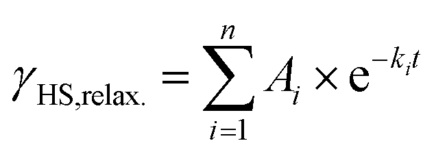
Even though [Fe(pypypyr)2] shows no thermal spin transition before thermal decomposition, we investigated the sample at low temperatures under irradiation with light to observe a potential LIESST effect. For this, we used SQUID magnetometry, UV/vis spectroscopy and NEXAFS spectroscopy. First, all three methods are described individually, before the results are compared and discussed in Sections 2.4–2.6.For an investigation of a potential LIESST effect, the powdered sample was placed in a sample holder with attached fibre optics. The sample was cooled to 5 K and the magnetic moment was observed by single-scan measurements in 10 s intervals. At 5 K, the signal was monitored without irradiation for 5 min. Afterwards, the sample was irradiated for 30 min with light at 545 nm, which notably led to an increase in the paramagnetic moment (see Fig. 3a), indicating a light-induced spin change. The resulting data was found to be best described by triexponential behaviour (see eqn (1); fitting parameters in Table 1), as monoexponential and, to a lesser degree, biexponential fits showed poor results (see ESI, Fig. S9†).
 | (1) |
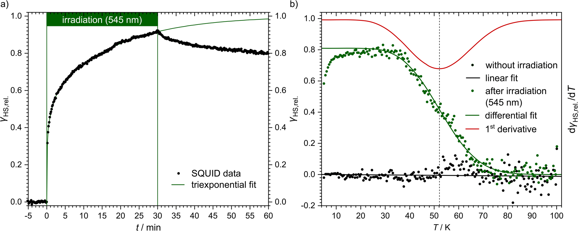 | ||
| Fig. 3 Magnetic susceptibility data of [Fe(pypypyr)2]. (a) Time dependence of the HS fraction (γHS,rel., black dots) over time during (t = 0–30 min) and after (t = 30–60 min) irradiation with 545 nm at 5 K. The HS fraction was calculated by fitting the data with a triexponential fit and dividing by the value at saturation. This does not reflect the fraction of bulk material that is in the HS state, but rather the fraction of molecules that can be switched with the used setup. (b) Temperature-dependence of the HS fraction (γHS,rel., green dots). Since the sample was heated directly after the relaxation from panel (a), the maximum HS fraction was set to 0.8, the final value (t = 60 min) in panel (a). The initial increase in the HS fraction is an artefact caused by zero-field splitting as well as the heat capacity of the sample holder. The HS state is stable up to 40 K. In the range from 40 to 70 K the sample relaxes thermally into the LS state. After reaching 100 K, the sample was cooled to 5 K and heated again without previous irradiation (black dots). Both data sets have been fitted using differential eqn (3) (data below 25 K were ignored) or a linear fit, respectively. The red line represents the first derivative of the Boltzmann fit for the determination of TLIESST ≈ 52 K. | ||
| A 1 | k 1/s−1 | A 2 | k 2/s−1 | A 3 | k 3/s−1 | γ HS,∞ | ||
|---|---|---|---|---|---|---|---|---|
| Excitation | SQUID | 0.457 ± 0.003 | (9.4 ± 0.1) × 10−4 | 0.21 ± 0.01 | (1.2 ± 0.1) × 10−2 | 0.33 ± 0.01 | (1.9 ± 0.6) × 10−1 | 1.000 ± 0.006 |
| NEXAFS | 0.096 ± 0.007 | (1.0 ± 0.3) × 10−2 | 0.06 ± 0.01 | (1.5 ± 0.7) × 10−1 | 0.15 ± 0.01 | 1.5 ± 0.2 | 0.888 ± 0.007 | |
| Relaxation | SQUID | 0.92 ± 0.01 | (3.5 ± 0.4) × 10−5 | 0.056 ± 0.004 | (2.8 ± 0.7) × 10−3 | 0.02 ± 0.01 | (2 ± 1) × 10−2 | — |
| UV/vis | 0.43 ± 0.04 | (1.3 ± 0.7) × 10−5 | 0.35 ± 0.04 | (2.8 ± 0.4) × 10−4 | 0.22 ± 0.02 | (7 ± 1) × 10−3 | — | |
| NEXAFS | 0.91 ± 0.04 | (1.3 ± 1.6) × 10−5 | 0.09 ± 0.04 | (1.4 ± 0.6) × 10−3 | — | — | — |
Higher-exponential behaviour suggests that there are multiple species involved, which could either be an intrinsic trait of the sample or induced by photoexcitation inhomogeneities. After 30 min of irradiation, 92% of the saturation value have been reached. However, this method cannot be used to determine accurately which fraction of the bulk material is in the HS state. Mainly, this is due to the unknown penetration depth of the light used for the excitation. As the sample has a very dark and deep colour, it is very likely to absorb a major part of the incoming light. Therefore, the fraction of molecules that comes into contact with light is probably very low. In fact, evaluation of the data led to a maximum observed paramagnetic susceptibility of 0.061 cm3 K mol−1 which corresponds to an HS fraction of ca. 2% (in relation to ca. 3.5 cm3 K mol−1 typically found for iron(II) HS compounds). The photo-excitation yield could probably be increased by reducing the sample mass,107 as this would lead to a higher surface-over-volume ratio. However, a complete spin-state conversion could neither be observed in vacuum-evaporated samples, which could be fabricated as thin, optically transparent films (see below). For evaluation and comparison purposes, we, therefore, decided to consider γHS,rel. as a fraction of the molecules in contact with light and set the saturation value of the triexponential fit to 100% relative HS fraction (see Fig. 3a).
After 30 min of irradiation, the light was switched off, causing an instantaneous increase in the signal, due to a rapid temperature decrease. Importantly, the light-induced HS state was found to relax slowly in the dark: 30 min after irradiation the paramagnetic moment was still at 87% of its peak value, which corresponds to about 80% relative HS fraction. The relaxation is again best described (see ESI, Fig. S9†) by a triexponential decay (see eqn (2); fitting parameters in Table 1).
 | (2) |
This fit results in a half time of τ = (290 ± 32) min, which is orders of magnitude higher than theoretically predicted for the title complex (see below).
After the excitation and relaxation measurements at 5 K, we investigated the thermal relaxation of the LIESST state upon increasing the temperature. To this end, the sample was heated to 100 K with a constant heat rate of 1 K min−1, one sweep without prior irradiation and one sweep directly after the previous relaxation measurement (Fig. 3b). Upon heating, the apparent magnetic moment first rises until about 25 K, which is an artefact related to zero-field splitting as well as the correction of the diamagnetic background and the different heat capacities of the sample and the sample holder. Based on the ending point of the above-described relaxation experiment, the highest paramagnetic moment is assigned to 80% HS (see Fig. 3b), although the real fraction is probably a little lower because ca. 20 min of tunneling relaxation have passed until this point is reached. Up to 40 K, no significant decrease in the paramagnetic moment is observed, which leads to the conclusion that the LIESST state is thermally stable to that point. Afterwards, the paramagnetic moment decreases until at approximately 70 K the LS state is fully recovered. Ignoring the influence of cooperative effects, this relaxation of the LIESST state during heating with a constant rate θ (see Fig. 3) can be described by the following differential equation:
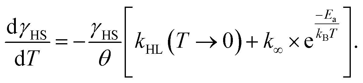 | (3) |
| Method | Condition | θ/(K min−1) | T LIESST/K | E a/cm−1 | k HL(T → 0)/s−1 | k ∞/s−1 |
|---|---|---|---|---|---|---|
| SQUID | — | 1.0 | 52 | 118 ± 7 | (0 ± 6.4) × 10−6 | (2.7 ± 0.6) × 10−2 |
| NEXAFS | Darkness | 1.2 | 52 | 124 ± 11 | (6.0 ± 1.6) × 10−5 | (3.6 ± 1.1) × 10−2 |
| Const. illum. | −0.6 | — | 170 ± 13 | (3.6 ± 1.8) × 10−4 | 2.1 ± 0.8 | |
| UV/vis | Intensity | 3.1 | 46 | 99 ± 32 | (7.6 ± 0.9) × 10−4 | (3.9 ± 3.3) × 10−2 |
| Area | 52 | 131 ± 53 | (6.7 ± 0.7) × 10−4 | 0.1 ± 0.1 |
Additionally, it is important to notice that differential eqn (3) assumes monoexponential behaviour for the tunneling rate. However, as shown above, the relaxation of the complex [Fe(pypypyr)2] does not appear to follow monoexponential but rather bi-, tri- or even higher exponential behaviour. This dramatically increases the error in the determination of the tunneling rate constant with this fit and may lead to a poor description of the low-temperature region. Nonetheless, the numerical solution to the differential equation appears to describe the experimental data above 25 K very well (see Fig. 3). Thus, we were able to determine the characteristic temperature TLIESST ≈ 52 K as the minimum of the first derivative of the fit.
For UV/vis absorption measurements, the title complex was prepared and investigated in three different ways: (i) finely dispersed in a KBr pellet, (ii) finely dispersed in a polystyrene (PS) film and (iii) deposited on quartz glass using physical vapour deposition (see Fig. 4a). This was done to investigate the effect of different degrees of cooperativity: a dispersion in KBr typically behaves similar to the bulk material, while the film on quartz glass behaves more like single molecules, despite the high thickness necessary for this method. Polystyrene films may behave either way or anything in between. Importantly, all three preparations led to similar spectra (see Fig. 4a, b and ESI, S11†), although the thin film on quartz glass has much better-resolved bands compared to the KBr pellet. The bands in the spectra of the PS film are of similarly high resolution, but two more pronounced shoulders appear at approximately 310 nm and 460 nm. Still, all spectra show a three-band feature with the main band at 688 nm and two much less intense bands at 620 nm and 578 nm. These three bands, as well as the band at 425 nm, are probably caused by CT transitions. Three further bands in the higher energy region (359 nm, 286 nm and 245 nm) are more likely the result of ligand-centred transitions (i.e. π → π* and n → π* transitions), as they are also present in the spectrum of the pure ligand dispersed in KBr (see Fig. 4a). This assignment is supported by careful analysis of TD-DFT-calculated excited states and the resulting simulated spectrum (see ESI, Section S3.5†).
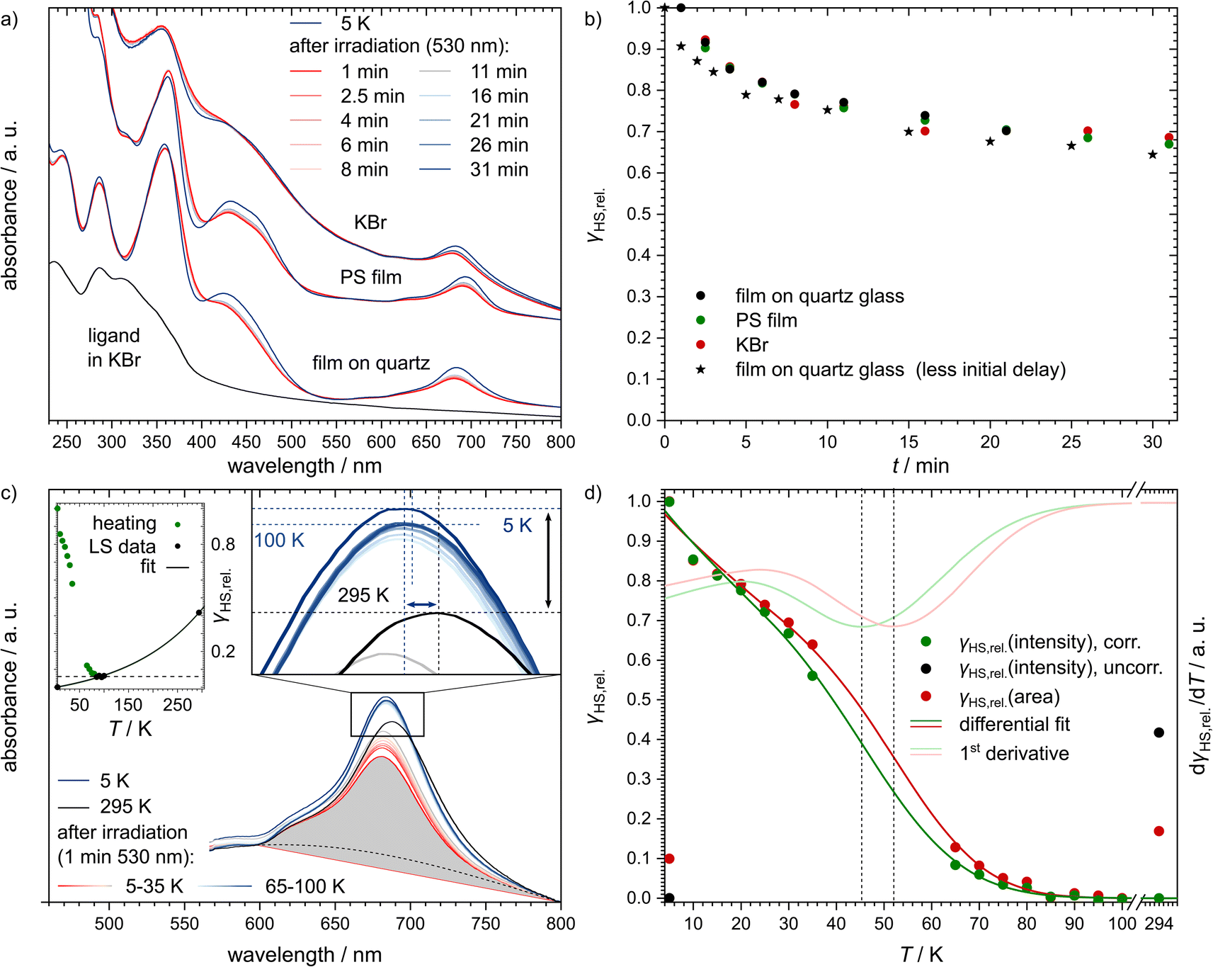 | ||
| Fig. 4 (a) UV/vis spectra of [Fe(pypypyr)2] for three different preparation methods: a thick film deposited on quartz glass via PVD, a dispersion in polystyrene and a dispersion in KBr. All samples were irradiated with a wavelength of 530 nm at 5 K and then observed in the dark for 30 min. Due to experimental limitations, the first spectrum after irradiation was taken 1 min after switching the light source off. Additionally, the UV/vis spectrum of the ligand dispersed in KBr at room temperature is shown for comparison. (b) Extracted HS fractions relative to the lowest observed absorbance of the band at ca. 684 nm for the three experiments shown in panel (a). The experiment on quartz glass was repeated with an optimised method that allowed the first measurement to be taken ca. 5 s after switching off the LED (black stars). (c) UV/vis spectra of [Fe(pypypyr)2] before irradiation at 295 K (black) and 5 K (dark blue), as well as after 1 min of irradiation using a 530 nm LED in intervals of 5 K (red to blue gradient) with a heat rate of approximately 3 K min−1. There is a gap from 40 K to 60 K since the spectra recorded at these temperatures had either much higher or lower absorbances that could not be corrected reliably (see ESI, Fig. S11b†). The black dotted line represents an assumption for how a pure HS spectrum might look like above 600 nm. The grey area marks the polygon area that was determined for all temperatures as a means to determine the HS fractions. For better visibility, the cusps of the spectra are shown in more detail. Here, the wavelength and intensity of the 294 K, 100 K and 5 K spectra are highlighted by dotted lines in the respective colour. Vertical and horizontal shifts between 294 K and 5 K are highlighted by a black and a blue arrow, respectively. The upper left inlay shows the HS fractions as determined from the intensities at the maximum of the CT band. The black dots represent the temperatures where 100% LS is expected (saturation at 6% HS highlighted by the dashed line). Those data points were fitted with a monoexponential fit that describes the apparent increase of the HS fraction due to thermal expansion (bigger version see ESI, Fig. S14b†). (d) Relative HS fractions of the switching molecules for the different temperatures determined by eqn (4) (green circles) after subtraction of eqn (7) to correct the data for the influence of the thermal expansion on the intensity of the CT band. The black circles show the uncorrected HS fractions before irradiation at 5 K and 294 K. As an alternate means, the HS fractions were determined based on the polygon areas below the spectra between 595 nm and 800 nm (red circles). Both data sets were then fitted using differential eqn (3) (dark green and red lines). The first derivatives of those fits (light green and red lines) then allow the determination of TLIESST ≈ 46 K and 52 K, respectively. | ||
After cooling the samples down to 5 K, no major changes in the spectra occurred. All bands increased slightly in intensity and the bands at 688 nm and 425 nm shifted to slightly higher energies (684 nm and 421 nm, respectively; the spectral change is highlighted by the arrows in Fig. 4c). This change cannot be attributed to a spin transition, but is rather a generally observed temperature-dependence and most likely caused by thermal compression of the LS structure. Similar changes in the bond lengths without a spin transition are well-known for Fe(II) coordination compounds.108,109 For example, in crystal structures of [Fe(terpy)2](ClO4)2·H2O, the Fe–N bond lengths decrease by up to 0.018 Å between 283–303 K (ref. 110) and 100 K (ref. 111) (see ESI, Table S4 and Fig. S10†). Extrapolation to 5 K leads to a potential decrease in bond lengths of up to 0.024 Å, which corresponds to ca. 12% of the change during spin transition. As described above, shorter bond lengths lead to a higher overlap of the metal- and ligand-centred orbitals, which results in a higher transition probability and thus higher intensity of the CT bands.
Next, we investigated the LIESST effect by illuminating the samples using a 530 nm LED for up to 30 min. However, 1 min of irradiation was found to yield the same spectrum as 30 min of irradiation. In agreement with the above results, the CT bands notably decreased in intensity after irradiation (see Fig. 4a).
Based on the described measurements, an exact evaluation of the HS fractions is only possible if spectra of the pure LS state and the pure HS state, both, are available. As [Fe(pypypyr)2] is pure LS over the complete observable temperature range, no pure HS spectrum is available to evaluate what fraction of molecules can be excited via irradiation at low temperatures. Indeed, the decrease in intensity is lower than expected, indicating that a non-negligible fraction of molecules did not switch. In contrast to the above SQUID measurements, penetration depth of the light source can be excluded from being an issue as all samples were transparent and one has observed that a large fraction of the light is passing through the samples. It may be worth noticing that 530 nm is right in the minimum of the absorbance of this compound with only wavelengths above 730 nm being absorbed less. Therefore, we repeated the experiment using an LED with a wavelength of 440 nm. However, this resulted in exactly the same spectra within 1 min and once again did not change after irradiation times of up to 20 min. The fact that light sources with a wavelength of 530 nm are as efficient as other wavelengths in the maxima of absorbance may be due to d–d transitions in that region that are much less intense due to being Laporte forbidden and thus not visible in the UV/vis spectra.
Another possible reason for an incomplete excitation may be the initially very fast relaxation we observed (see below), since our initial setup involved the removal of the LED that took about 1 min after irradiation before the first spectrum was measured. Therefore, we improved our experiment with an automatised pneumatic removal of the LED, thereby lowering the time between irradiation and measurement to ca. 5 s. However, this did not change the results drastically (see Fig. 4b). We further hypothesised that the measurement beam of the spectrometer may induce a reverse-LIESST effect112,113 and thus force partial relaxation. To investigate this, we repeated the measurements varying the intensity of the measurement beam between 10% and 1000% of the original intensity. While this did lead to slightly different spectra, the differences caused by different beam intensities were consistent for all spectra at 300 K and 5 K before and after irradiation, thus proving that the HS fraction does not depend on the intensity of the measurement beam and no reverse-LIESST occurs (see ESI, Fig. S12†).
The relative fraction of HS molecules was determined as follows. We evaluated the spectra using eqn (4),114 thus obtaining HS fractions relative to the maximum observed HS fraction. For this, the maximum absorbances of the band at around 684 nm were used (OD![[small nu, Greek, tilde]](https://www.rsc.org/images/entities/i_char_e0e1.gif) (x), with x = T or t, depending on the measurement) with the spectrum at 5 K before irradiation assumed to be pure LS (OD(LS)) and the spectrum 5 s after irradiation (OD(HS)) set to be 100% of the switchable molecules. This resulted in HS fractions relative to the highest observed HS fraction instead of absolute values.
(x), with x = T or t, depending on the measurement) with the spectrum at 5 K before irradiation assumed to be pure LS (OD(LS)) and the spectrum 5 s after irradiation (OD(HS)) set to be 100% of the switchable molecules. This resulted in HS fractions relative to the highest observed HS fraction instead of absolute values.
 | (4) |
Assuming a CT band of the HS state as shown in Fig. 4c (black dotted line), one finds that approximately 40% of the molecules are observed in the metastable LIESST state at maximum.
In order to monitor the relaxation following optical excitation, we first investigated the stability of the excited state at 5 K by measuring further spectra over 180 min after the irradiation (see Fig. 6 and ESI, S13† for more details). We found that the HS fraction decreases quickly in the first 5 min, before the relaxation slows down. Similarly to the SQUID results described above, the relaxation is best described using a triexponential fit using eqn (2) (fitting parameters in Table 1). According to this fit, 50% of the initially excited molecules have relaxed after (80 ± 14) min.
We also investigated the thermal stability of the excited state by increasing the temperature to 100 K with an average heat rate of about 3 K min−1 (see eqn (5) and ESI, Fig. S14a†).
| t = θ−1 × (T − T0) = 0.322 min K−1 × (T − 5 K), θ = 3.11 K min−1 | (5) |
Up to 20 K, the HS fraction determined by eqn (4) closely resembled the isothermal behaviour at 5 K (see Fig. 4c). However, at 25 K the relaxation started to accelerate. Unfortunately, we were not able to evaluate the five spectra between 40 K and 60 K as these spectra showed a reproducible discontinuity with intensities shifted to much higher and lower (i.e. negative absorbances) intensities (spectra and resulting HS fractions, see ESI, Fig. S11†). We regularly experience this phenomenon with UV/vis spectra at temperatures close to T1/2 or TLIESST, although the shift is especially high for this compound.
At about 85 K, the relaxation reaches a saturation (see right inlay of Fig. 4c, blue dotted, horizontal line in the middle or black points in the left inlay), i.e., the LS intensity of 5 K is not totally recovered. Using eqn (4), the residual HS fraction is determined to be 6%. However, this observation is ascribed to a temperature-dependent intensity decrease of the low-spin band, rather than an actual HS fraction. This is supported by the fact that the intensity of the low-spin band is even lower at room temperature (see Fig. 4c, black arrow). Moreover, there is a shift of the maximum of this band (see Fig. 4c, blue arrow). In order to account for the intensity decrease of the low-spin band, the relative HS fraction determined from eqn (4) is corrected by a temperature-dependent term δT:
| γHS,rel. = γHS,rel.,corr. + δT. | (6) |
For the purpose of fitting the data and thus being able to determine TLIESST, we determined δT by fitting the data points that are presumably completely LS (see Fig. 4c, black points in the left inlay) with a monoexponential fit:
 | (7) |
The relative HS fractions were then corrected by subtracting the fitted function for δT to obtain only the contribution from light-induced spin-crossover γHS,rel.,corr. (see Fig. 4d, green points). However, trying to fit the corrected data with the differential eqn (3), we found that the function poorly describes the initially accelerated relaxation (see Fig. 4d, green line). This is probably caused by the fact that such a fit includes a monoexponential tunneling term, whereas, as shown above for UV/vis spectroscopy and SQUID magnetometry, the isothermal tunneling relaxation of [Fe(pypypyr)2] does not appear to follow monoexponential behaviour. Nevertheless, the fit does describe the data at higher temperatures (i.e., above 20 K) well enough to warrant the determination of TLIESST ≈ 46 K using its first derivative (see Fig. 4b, red line).
For this investigation, powder of the sample was stamped into indium foil and cooled down from 300 K to 8 K. The spectrum at 300 K showed only one feature as expected for the sample being in the LS state (see Fig. 5a). At the lowest temperature of 8 K, however, a second feature began to rise due to irradiation with soft X-rays used for the measurement (see Fig. 5a, grey spectra and points). This is known as the SOXIESST (soft X-ray-induced excited spin state trapping) effect.117–119 Under constant illumination with a wavelength of 520 nm, the second feature became even more prominent due to LIESST excitation (see Fig. 5a, red spectra and black points). The spectral shape was analysed to give relative HS fractions. The resulting excitation curve (see Fig. 5a, green line) is, similar to the results from SQUID magnetometry, best described by triexponential behaviour (using eqn (1); parameters in Table 1). Notably, this differs from all known examples of spin-crossover systems where the excitation of the metastable high-spin state by light irradiation follows monoexponential characteristics.119 We assume that this obervation is due to the fact that the HS state of the title complex is distorted along several internal coordinates with respect to the LS configuration (see below) and that different species exhibiting different degrees or types of molecular distortions exist. These individual species thus undergo excitation to the respective HS states at different rates.
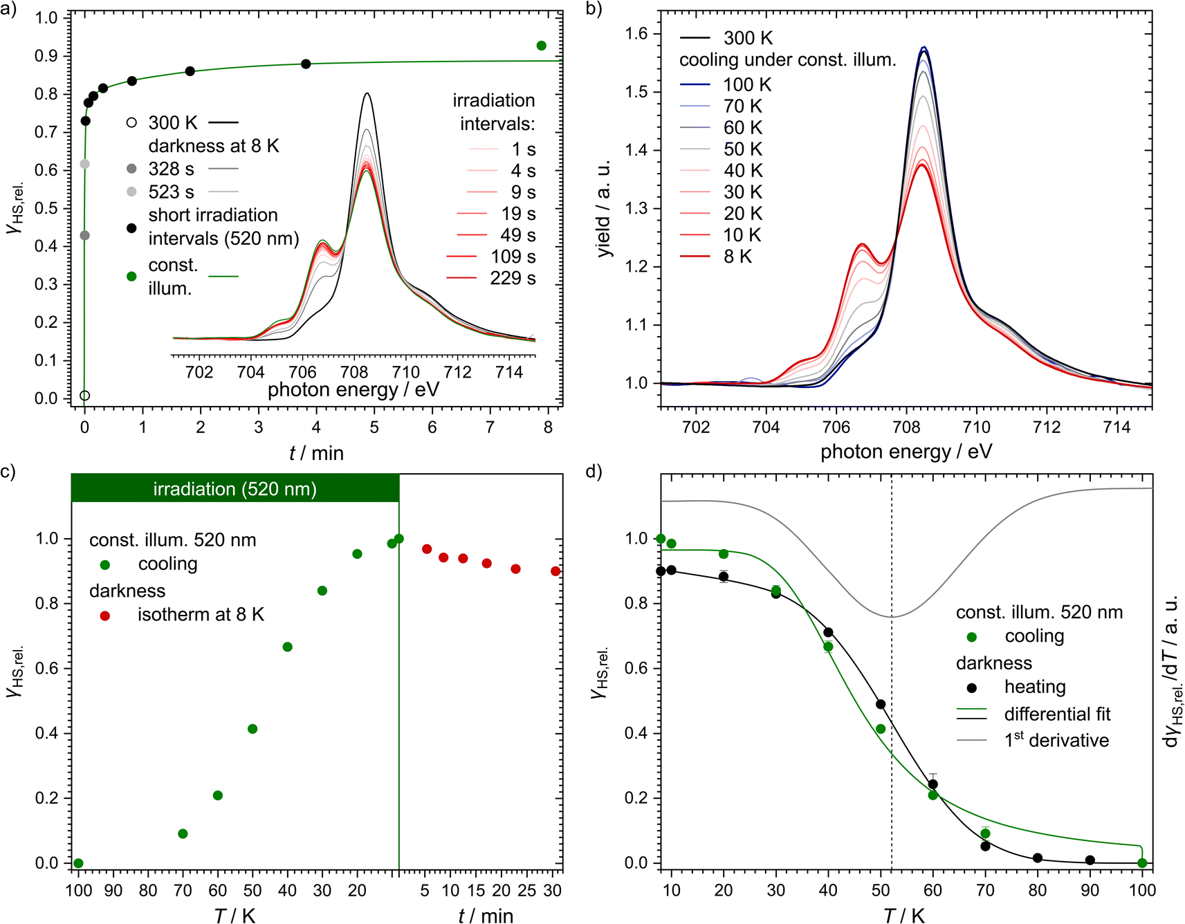 | ||
| Fig. 5 (a) Plot of the HS fractions extracted from NEXAFS spectra at 300 K (black empty circle; black spectrum), upon reaching 8 K and after 6.5 min in darkness at that temperature (grey circles and spectra), after several short intervals of illumination (black circles; red spectra; cumulative irradiation time is given) and during constant irradiation with 520 nm (green circle and spectrum). The cumulative irradiation interval data were fitted using a triexponential function (green line). A comparison with mono- and biexponential fits is available in the ESI (Fig. S19†). The inlay shows the corresponding NEXAFS spectra of [Fe(pypypyr)2], which were smoothened for presentational purposes using a LOESS regression (for exemplary raw data see ESI, Fig. S18†). (b) NEXAFS spectra of [Fe(pypypyr)2] powder stamped into indium foil at 300 K in darkness (black) and during cooling from 100 K to 8 K under constant illumination with 520 nm (gradient blue to red). The spectra during heating in darkness are available in the ESI (Fig. S21b†). (c) Extracted HS fractions when cooling the sample under constant illumination (520 nm) from 100 K down to 8 K (green). After reaching the lowest temperature, the laser was switched off and the isothermal relaxation was observed (red). (d) HS fractions determined from the temperature-dependent NEXAFS spectra in relation to the highest observed HS fraction. The sample was heated to 100 K (black) and the resulting curve fitted with eqn (3). Determining the first derivative of the fit for the heating curve (grey) allowed us to ascertain a TLIESST value of 52 K. For comparison, the cooling curve from panel (c) is shown as well (green). In contrast to the heating curve, it was fitted using a modified function to also include the excitation rate (see eqn (8)). | ||
In a different experiment, we started at 100 K and cooled the sample down to 8 K under constant illumination with a wavelength of 520 nm (see Fig. 5b). At around 80 K, the LS feature started to decrease in intensity whereas the HS feature increased. The extracted HS fractions (see Fig. 5c and d, green points) show typical Boltzmann behaviour with a final value at 8 K that is ca. 10% higher than in the previous experiment. This can be explained by the inhomogeneity of the powdered sample's surface. To be able to compare these data with the results from the SQUID and UV/vis experiments described above, this spectrum is assigned to a relative HS fraction of 100%. However, comparison with NEXAFS data of the fully switching complex [Fe(H2B(pz)2)2(bipy)] reveals that the LIESST excitation is indeed incomplete with only about 48% of the molecules being in the HS state (see ESI, Section S3.6 and Fig. S17†).
After this experiment, we investigated the relaxation in the dark. To this end, the laser was turned off after reaching the lowest temperature. After 30 min, ca. 90% of the initially excited molecules remained in the HS state (see Fig. 5c, red points). Here also, monoexponential behaviour cannot explain the decrease of the HS fraction (see ESI, Fig. S20†). Instead, we applied a biexponential fit using eqn (1) with A3 = 0 (see Fig. 6; fitting parameters in Table 1) as too few data points were measured to obtain a meaningful triexponential fit. This fit resulted in an extrapolated half time of the metastable HS state of [Fe(pypypyr)2] of (781 ± 412) min.
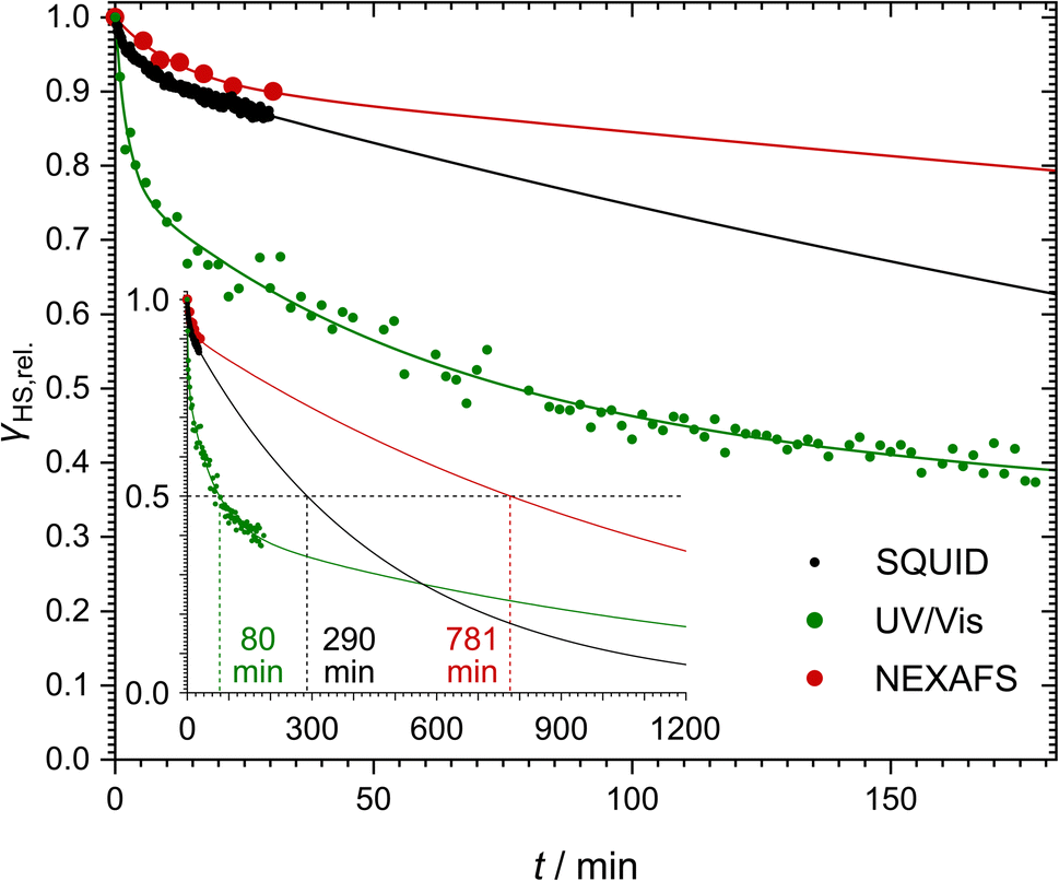 | ||
| Fig. 6 Comparison of the relaxation of the metastable LIESST state after illumination in darkness at constant low temperature (5 K for SQUID magnetometry and UV/vis spectroscopy; 8 K for NEXAFS spectroscopy). The data points are given in black (SQUID), green (UV/vis spectroscopy) and red (NEXAFS spectroscopy). The respective tri- (SQUID and UV/vis) or biexponential (NEXAFS) fits are given in the same colour. All data are given as relative HS fractions compared to the maximum observed HS fraction to allow comparison of the different methods. The inlay shows a wider time span to determine half times for each fit as the times when 50% of the initially excited molecules have relaxed. | ||
Directly after the relaxation experiments, the sample was heated in the dark with a heat rate of ca. 1.2 K min−1 (see Fig. 5d, black points). From 30 K onwards the HS fractions closely resemble the data collected during cooling under constant illumination, just slightly shifted to higher temperatures, with the sample almost completely relaxed at ca. 70 K. A fit based on numerical integration of eqn (3) (fit parameters in Table 1) and its first derivative (see Fig. 5d, black and grey line, respectively) provided a characteristic temperature TLIESST of approximately 52 K in this experiment. In an effort to fit the cooling curve under constant illumination as well, eqn (3) was modified to include the excitation rate described by the rate constant kexc.:
 | (8) |
Similarly to the relaxation, the excitation is also assumed to follow monoexponential behaviour in this equation, which is in contrast to the above-described experimental observations. With a fixed kexc. of 0.01 s−1, which marks the lower limit of the experimentally observed rate constants, the parameters given in Table 2 are obtained. The above-mentioned simplified assumptions, as well as the fact that k∞ is in reality not independent of the temperature, explain the differences between the parameters obtained for the two curves during heating and cooling, respectively. Furthermore, eqn (3) and (8) assume Arrhenius behaviour over the whole temperature range between 5 K and 100 K. However, distinctly non-Arrhenius behaviour has been observed in a temperature range between 25 K and 100 K for [Fe(terpy)2]2+, which strongly resembles the title compound structurally.40 Due to these oversimplifications, the observed deviations in the fit parameters are to be expected.
2.4 Relaxation rates
Comparing the low-temperature relaxation behaviour observed with the three spectroscopic methods described above, we consistently found non-monoexponential behaviour in all experiments (see Fig. 6). One potential explanation for these results may be photoexcitation inhomogeneities. As described above, inhomogeneous excitation is very likely in our SQUID magnetometric setup due to the deeply coloured sample, which leads to shallow penetration of the light used for the excitation. This hypothesis could even hold for the NEXAFS experiments: the green light of the LED comes from a different direction than the X-rays. Consequently, there could be probed regions with higher or lower green-light illumination. However, the same does not hold for the UV/vis spectroscopic results. Here, all samples were transparent, thus eliminating penetration depth as a cause for excitation inhomogeneities. Furthermore, the LEDs were pneumatically moved directly in front of the measurement beam for the irradiation. As such, irradiation and probing were performed from the exact same angle and direction, thereby guaranteeing that all probed molecules were also irradiated beforehand. In consequence, photoexcitation inhomogeneities cannot be the only reason for the non-monoexponential relaxation behaviour. A different explanation based on the molecular structure of the complex is proposed further below (see Section 2.5).Comparison of the determined half times reveals a difference of up to one order of magnitude (see Fig. 6). Our UV/vis spectroscopic investigation of a thin film on quartz glass yielded the shortest half time of (80 ± 14) min. Extrapolation of the SQUID magnetometric and NEXAFS spectroscopic experiments on bulk material, on the other hand, led to half times of (290 ± 32) min and (781 ± 412) min, respectively. Fits of all three isothermal relaxation curves led to similar tunneling rate constants kHL(T → 0), with the lowest rate constant in the regime of 10−5 s−1 and the highest rate constant in the range of 10−3–10−2 s−1 (see Table 1).
The difference between the half times may partially be explained by the fact that we only measured the half time directly in our UV/vis spectroscopic experiment, whereas for the other experiments, it had to be derived from the fit function. Moreover, the slightly slower relaxation found in the NEXAFS experiments compared to the SQUID data may potentially be caused by the SOXIESST effect partially counteracting the tunneling relaxation. Still, the noteable difference between the UV/vis spectroscopic results and the other two experiments is also very apparent in the experimental data points (see Fig. 6) and thus not caused by imprecise fits. Instead, the data suggest that the complex relaxes slower in the bulk phase compared to thin films and dispersions (compare Fig. 6 and 4b).120 The main difference seems to be that a portion of the molecules relaxes much faster in thin films, leading to much steeper decay characteristics in the early stages of the isotherm. While the fit parameters (see Table 1) show very similar relaxation rates (ki in Table 1), the species with the lowest relaxation rate makes up for over 90% of the bulk samples, whereas it only accounts for 43% of the thin film, the two species with a much higher relaxation rate being only slightly less represented (35% and 22%, respectively). In conclusion, the relaxation seems to be strongly influenced by solid-state effects, which presumably depend on the initial HS fraction. However, based on the estimations presented above, the initial absolute HS fraction before relaxation is nearly identical in the NEXAFS and UV/vis spectroscopic experiments (48% and 40%, respectively). As such, this dependency alone cannot explain the drastic difference between the two relaxation curves. A different explanation may be found in the difference between bulk material and thin films: the fraction of near-surface molecules, where solid-state effects are less pronounced, increases with decreasing film thickness. Consequently, the experiments on the thin film show a higher fraction of the less inhibited species and in turn a faster relaxation. This appears to be true even for dispersions in polystyrene or KBr.
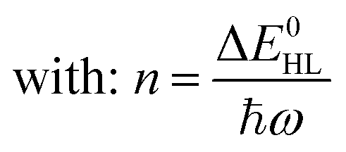
Notably, despite the differences in the results, all experiments show unambiguously and independently that the excited HS state after irradiation with light is metastable at low temperatures for comparatively long times (in the regime of hours). These results are in stark contrast with the expectations based on the inverse energy gap law.30,33,38 As predicted theoretically,121 it was found that the relaxation of the HS state to the LS state is thermally activated above ca. 100 K, but nearly independent from the temperature below ca. 50 K. In this low-temperature region, the process is dominated entirely by tunneling. The tunneling rate constants of iron(II) spin-crossover complexes were found to depend mainly on the energy gap ΔE0HL between the potential wells of the two states: small energy gaps result in very small rate constants (large lifetimes) that increase (decrease) exponentially with increasing ΔE0HL. Since the energy gap has a direct influence on the spin transition temperature T1/2 as well, this model explains why nominal LS compounds with high ΔE0HL and T1/2 typically have extremely large tunneling rate constants. Correspondingly, half times of the metastable LIESST state are expected to be in the regime of micro- or nanoseconds. To validate this statement, we applied a DFT-calculated energy gap of ΔE0HL = 3300 cm−1 for [Fe(pypypyr)2] (see ESI, Table S1†) to eqn (9) to estimate a tunneling rate constant. To this end, ΔE0HL was transformed into the reduced energy gap n (see eqn (10)), assuming a typical vibrational frequency of the active vibration according to the single-mode model for spin-crossover compounds of ℏω = 250 cm−1.30,40 Furthermore, average values for the Huang–Rhys factor (S = 45) and the electronic coupling matrix element (βHL = 150 cm−1) were assumed.30,40 Thereby, a rate constant of ca. 1.95 × 10⁶ s−1 can be expected for [Fe(pypypyr)2], which corresponds to a half time of 355 ns.
 | (9) |
 | (10) |
For [Fe(pypypyr)2], there is some uncertainty in this estimate due to the fact that no thermal spin transition could be observed for this compound. Thus, no experimental determination of T1/2 and ΔE0HL was possible. Hence, a more conservative approach would be using 510 K (the temperature up to which the experiments show no indication of a spin transition) as the lower limit for T1/2 and then calculating ΔE0HL,min (see eqn (11) with ΔS = 5 cm−1 K−1).33
| ΔE0HL ≈ ΔH0HL = ΔS0HLT1/2 | (11) |
Applying eqn (9) with S = 50 (upper limit typically observed) leads to kHL,min = 7.54 × 10² s−1 or a half time of 919 μs.
These theoretically expected tunneling rate constants based on the inverse energy gap law are at least four and up to eleven orders of magnitude higher than the rate constants obtained from fitting the experimental data measured for [Fe(pypypyr)2] with three independent methods.
In an effort to explain the described behaviour of the title compound [Fe(pypypyr)2], we searched for suitable precedence. To the best of our knowledge, there are only two other nominal LS compounds for which a comparable lifetime of the metastable LIESST state has been observed: when dispersed in various matrices, [Fe(terpy)2]2+ (terpy = 2,2′:6′,2′′-terpyridine), a nominal LS compound, starts to show a light-induced spin transition.39 While its low-temperature tunneling rate constant is about 103 s−1 when dispersed in KBr, dispersion in [M(terpy)2](PF6)2 (M = Zn, Mn, Cd) leads to a decreased rate constant of ca. 10−5 s−1.40 The second group of complexes is based on macrocyclic ligands that bind as tetradentate ligands in the LS state ([Fe(LN5)(CN2)]·H2O; e.g. LN5 = 2,13-dimethyl-3,6,9,12,18-pentaazabicyclo[12.3.1]octadeca-1(18),2,12,14,16-pentaene, but other ring sizes have also been explored).41,43 However, upon irradiation at low temperatures a paramagnetic HS compound with an unusually high critical temperature is obtained. This was theorised to be caused by a change in coordination number from the octahedral LS complex to a heptacoordinated HS complex. Later on, crystal structure analysis revealed that this theory is indeed correct. However, instead of coordinating solvent molecules, the ligand itself rearranges upon spin transition and coordinates with all five N-donor atoms instead of as a tetradentate ligand. The high structural arrangement necessary may also explain the unusually high LIESST temperature.41–45 In contrast, [Fe(pypypyr)2] shows the same effect without having to be dispersed in a matrix. Also, the trace amounts of solvents included in the sample cannot explain the observed behaviour, even if they lead to a change of the coordination number, and there are no other free donor atoms that could lead to a change of the coordination number. As a result, a closer look at the coordination sphere of [Fe(pypypyr)2] and comparison with the above mentioned complexes is necessary to understand the observed behaviour.
2.5 Molecular distortions accompanying spin-crossover
The differing relaxation rates depending on a matrix observed for [Fe(terpy)2]2+ had already been shown for [Fe(bipy)3]2+ and have been attributed to a modulation of ΔE0HL depending on the lattice pressure.40 However, the vast difference in the tunneling rate constant of [Fe(terpy)2]2+ in different matrices cannot be explained by this effect. Instead, Hauser et al. proposed a breakdown of the single-mode model of the spin transition: dependency of the spin transition on more than one normal mode is expected to increase the activation barrier and lower the rate constant for the tunneling process. They found evidence for this theory in DFT-calculated structures of the two spin states that showed a much more drastic increase in bond length between the metal centre and the central pyridine compared to the bonds between the metal centre and the outer pyridines (0.28 Å for Fe–Npy,centralvs. 0.20 Å for Fe–Npy,outer).40 In addition to this asymmetric bond elongation, the calculated structures showed a decrease of the bite angles εi (LS: 81°, HS: 75°; see ESI, Table S12†). Based on this, it may be worth investigating the structure of the two spin states of [Fe(pypypyr)2] to understand its unusual behaviour.To this end, we examined the DFT-calculated structures of the two spin states (see Fig. 7b and c), as well as two experimental crystal structures (see Fig. 7a and d). While the LS state was experimentally available, the HS state can only be obtained at low temperatures after LIESST excitation for a limited lifetime and is therefore not amenable to single-crystal structure analysis. Instead, we synthesised and crystallised the zinc(II) analogue. It has been shown multiple times that Zn(II) complexes often have a similar molecular structure to the Fe(II) HS state or are even isotypic.104,105,122–125 However, we were unable to grow crystals without residual solvent molecules in both cases (statistically distributed solvent that could not be identified in the Fe(II) structure and one equivalent of DCM (dichloromethane) in the Zn(II) structure; see CCDC-2233051 for [Fe(pypypyr)2] and CCDC-2233052 for [Zn(pypypyr)2], as well as ESI, Section S3†). The solvent definitely influences the packing of the individual molecules and intermolecular interactions between them, making it impossible to compare cooperative effects between the two spin states (a detailed description of the crystalline packing can be found in ESI, Section S3.8.1†). However, the molecular structure itself does not appear to be influenced by the solvent in any major way, as is apparent when comparing the Zn(II) crystal structure with the calculated structure of Fe(II) in the HS state (see Fig. 7d and c). Assuming that the Zn(II) structure is isotypic to the Fe(II) HS structure, we can now also exclude a change of the coordination number to be the cause for the spin transition, as we found no evidence for this effect in the crystal structure despite it containing solvents.
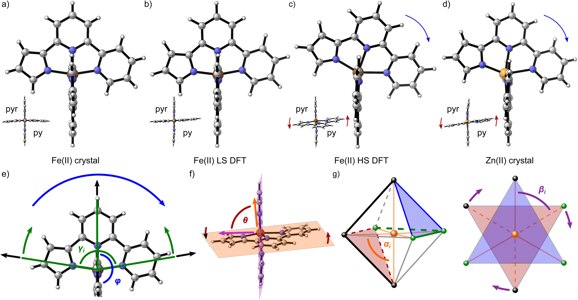 | ||
| Fig. 7 (a–d) Molecular structures of [Fe(pypypyr)2] (a–c) and [Zn(pypypyr)2] (d) as calculated using DFT (b and c) and found in single-crystal structures (a and d). All structures are shown along the x-axis (frontal view) to visualize the tilt of one of the two ligands in the yz-plane that appears in the Fe(II) HS state and the Zn(II) complex (the other ligand behaves identically in the xz-plane). Additionally, all structures are shown along the intersecting line of the two ligand planes (top view) to visualize the angle θ between them. Elements are colour-coded according to red-brown: Fe; orange: Zn; blue: N; grey: C; white: H. In the frontal view, the pyrrole of the second ligand is located in the rear. In the top view, pyr and py indicate the location of the pyrrole and the outer pyridine, respectively, in both ligands. Both crystal structures contain solvent molecules (not shown). The blue arrows in panels (c) and (d) highlight the in-plane tilt of the ligands and the red arrows indicate the twisting mode. (e–g) Schematic overview of the observed distortion modes and the corresponding parameters. (e) A section of [Fe(pypypyr)2] is shown along the x-axis (frontal view). Upon spin transition, the Fe–N bond lengths increase (black arrows). For tridentate, planar ligands, a bending mode can be observed (green arrows) and quantified by the decrease of the two intraligand trans-N–Fe–N angles γi. A potential tilt of one ligand relative to the other (blue arrow) results in a decrease of the interligand trans-N–Fe–N angle φ. (f) The complex [Fe(pypypyr)2] is shown along the intersecting line of the two ligand planes (top view). A twisting mode of the two ligands relative to each other (red arrows) can be quantified by the angle θ between the normal vectors of the two ligand planes (indicated in orange and violet). (g) Octahedral and trigonal antiprismatic (view perpendicular to one set of two trigonal planes between three ligand donor atoms; planes indicated in red and blue, respectively) display of the complex [Fe(pypypyr)2] (the two ligands are represented by black or green spheres and lines, respectively). Distortion of an octahedral complex is conventionally described by the deviation of the cis-N–Fe–N angles αi (orange) from 90°. Distortion of the trigonal antiprismatic geometry (trigonal planes staggered) towards a trigonal prismatic geometry (trigonal planes eclipsed; indicated by purple arrows) is conventionally described by the deviation of the torsion angles βi between two donor atoms in different trigonal planes from 60°. | ||
Comparing the various structures, we found that the bond elongation upon spin transition is very different for the three nitrogen atoms of the pypypyr− ligand: while the bond between iron and pyrrole only increases by ca. 0.13 Å in the DFT-calculated structures (0.11 Å in the crystal structures), the bond between iron and the outer pyridine increases by 0.31 Å (see Table 3) and even more in the two crystal structures (0.38 Å). The resulting difference in elongation is 0.18 Å (0.27 Å in the crystal structures) compared to the 0.08 Å found for [Fe(terpy)2]2+. These findings can also be quantified by the parameter ζ:
 | (12) |
 | (13) |
| LScryst | LScalc | HScalc | Zncryst | Δcalc | Δcryst | |
|---|---|---|---|---|---|---|
| d py,c/Å | 1.89 | 1.91 | 2.16 | 2.13 | 0.25 | 0.24 |
| d py,o/Å | 1.97 | 1.99 | 2.30 | 2.34 | 0.31 | 0.38 |
| d pyr/Å | 1.96 | 1.97 | 2.10 | 2.07 | 0.13 | 0.11 |
| ζ/Å | 0.22 | 0.17 | 0.46 | 0.65 | 0.29 | 0.43 |
| ξ/° | 35.8 | 35.6 | 62.9 | 64.1 | 27.3 | 28.3 |
| φ/° | 179.1 | 179.3 | 155.6 | 167.3 | −23.7 | −11.8 |
| θ/° | 89.7 | 84.7 | 86.6 | 80.2 | 1.9 | −9.5 |
| Σ/° | 77.3 | 79.4 | 143.0 | 141.7 | 64.7 | 64.4 |
| Θ/° | 255.5 | 256.3 | 527.7 | 484.5 | 271.4 | 229.0 |
This parameter describes the deviation of the Fe–N bond lengths from the average and increases to more than double from 0.17 Å (0.22 Å) in the LS state to 0.45 Å (0.65 Å) in the HS state of [Fe(pypypyr)2]. Contrarily, ζ decreases slightly from 0.26 Å in the LS state to 0.21 Å in the DFT-calculated HS structure of [Fe(terpy)2]2+. In summary, [Fe(pypypyr)2] shows an even more pronounced disparity in bond elongation compared to [Fe(terpy)2]2+.
Similar to [Fe(terpy)2]2+ (see ESI, Table S12†), we also observe a drastic change in the bite angles of the tridentate ligands between the structures of the two different spin states. In the LS state, all bite angles are approximately 81°, both in the single-crystal structure and the DFT-calculated structure, in close agreement with [Fe(terpy)2]2+. However, in the single-crystal structure of [Zn(pypypyr)2]·DCM and the DFT-calculated structure of the Fe(II) complex in the HS state, the two different bite angles vary tremendously due to the asymmetry of the ligand: while the bite angle between pyrrole and the central pyridine barely changes upon spin transition (Fe(II) HS: 77.0°; Zn(II): 78.0°), the bite angle between the two pyridines decreases drastically (Fe(II) HS: 71.6°; Zn(II): 71.2°). For better comparability, we define the intraligand trans-N–Fe–N angle γi, which is equal to the sum of the two adjacent bite angles of a single ligand (see Fig. 7e). The bending parameter ξ is then given as the sum of the differences between 180° and the γi values:
 | (14) |
The introduction of this parameter clearly shows that the overall distortion caused by the additional bending mode, albeit asymmetrical, is even more pronounced in [Fe(pypypyr)2] (ca. 28°) compared to [Fe(terpy)2]2+ (ca. 22°).
While the asymmetric bond elongation and the additional bending mode are both more prominent in [Fe(pypypyr)2] than in [Fe(terpy)2]2+, this is not sufficient to explain the drastically enhanced stability of the LIESST state. However, there are two additional independent distortion modes: an in-plane tilt of the ligands towards the pyridine side (see Fig. 7c–e: blue arrows) and a twisting mode of the two tridentate ligands around the central pyridine–pyridine axis relative to each other (see Fig. 7f, c and d: red arrows).
The in-plane tilt of the ligands can be quantified by the interligand trans-N–Fe–N angle φ between the central pyridines (see Fig. 7e). For [Fe(terpy)2]2+, this parameter barely changes upon spin transition (LS: 179.8°, HS: 179.6°). While φ is very similar for [Fe(pypypyr)2] in the LS state (179.1°, see Table 3), it decreases drastically down to 167.2° in the Zn(II) structure. Notably, the deviation from 180° is even higher in the calculated Fe(II) HS structure with an angle of φ = 155.6°. This distortion is more in line with results often found for derivatives of [Fe(bpp)2]2+ (bpp = 2,6-bispyrazol-2-ylpyridine).126–128 Here, φ decreases down to 154° in the HS state, with angles below 172° considered a strong distortion.126,129 Thereby, the angle in the calculated Fe(II) HS structure approaches the highest observed distortion in the literature. We propose that this high distortion may be the main reason for the unusually high lifetime of the LIESST state of [Fe(pypypyr)2]. In the first survey of the Jahn–Teller distortion parameters for [Fe(bpp)2]2+ complexes, complexes with high distortion (φ < 172°) did not show spin-crossover but instead were in the HS state across the investigated temperature range, in contrast to other complexes that were very similar in structure except for a lesser distortion of the HS state. It was hypothesised that a strong structural rearrangement necessary to overcome high differences in distortion between the two spin states is not possible against a rigid lattice in the solid phase, thus essentially trapping the molecule in the HS state kinetically.129,130 While several complexes have been found in the meantime that show spin transition despite stronger distortion than initially proposed, all of those examples still show inhibition of the spin transition in the form of hysteretic transition behaviour.127,128,131,132
The twisting mode of the two ligand planes can be expressed by the angle θ between the normal vectors of the two ligand planes (see Fig. 7f, c and d: red arrows). For [Fe(terpy)2]2+ in both spin states (LS: 89.8°, HS: 88.6°) and [Fe(pypypyr)2] in the LS state (89.7°), this parameter is very close to 90°. In contrast, the HS complex shows significant distortion (θ = 80.2°) (see Fig. 7c). Compared to other published complexes, however, this distortion mode is rather insignificant (i.e., values down to 59° in the HS state have been observed for derivatives of [Fe(bpp)2]2+, with angles below 76° considered to be low).129
In summary, [Fe(pypypyr)2] shows four independent modes of distortion, two of which are not observed for [Fe(terpy)2]2+, the only other LS compound that has been observed in the LIESST state, albeit only when dispersed in matrices.
This high degree of distortion also becomes apparent from the parameters Σ and Θ that are conventionally used to quantify the overall distortion of octahedral complexes.133,134 The former represents the deviation of the cis-N–Fe–N angles αi from a perfect octahedron (see eqn (15) and Fig. 7g), whereas the latter is a measure for the distortion towards a trigonal prismatic coordination sphere, defined by the torsion angles βj between neighbouring nitrogen atoms on opposing trigonal faces of the octahedron (see eqn (16) and Fig. 7g). Unlike the above-described modes of distortion, these parameters are not independent, but rather a result of the four types of distortion considered above.
 | (15) |
 | (16) |
For the parameter Σ, the difference between the two spin states of [Fe(pypypyr)2] is within the expected range observed in similar complexes (for details, see ESI, Section S3.8†). The trigonal distortion parameter Θ, on the other hand, has been shown to be dependent on the type of ligand: LS complexes with two tridentate ligands typically have distortion angles between 200° and 300° ([Fe(terpy)2]2+: 273.9°; bpp complexes: 270–316°) and HS complexes exhibit angles between 450° and 600° (bpp complexes: 453–559°).129,135 The difference between the two spin states in [Fe(bpp)2]2+ complexes with SCO behaviour is typically 151–192°.129 In comparison, the LS state of [Fe(pypypyr)2] appears to be relatively undistorted with little difference between the single-crystal structure and the DFT-calculated structure (255.5° and 256.3°, respectively). The Zn(II) structure, on the other hand, shows medium distortion (484.5°), leading to a very high difference ΔΘ of 229.0° between the single-crystal structures of the Zn(II) complex and the Fe(II) complex in its LS state. However, according to our calculations, an even stronger distortion is expected in the Fe(II) HS state (Θ = 527.7°; ΔΘ = 271.4°). Indeed, high deviation between the Zn(II) and Fe(II) HS structures is not unprecedented (see ESI, Table S11†).104 With Θ increasing by more than 100% upon spin transition, the enormous structural differences between the two spin states become apparent. This typically coincides with a high stability of the LIESST state.134,136
Based on these findings, we propose that the unusually high lifetime of the LIESST state of [Fe(pypypyr)2] is a result of kinetic inhibition of the spin transition caused by unusually high structural differences between the two spin states. Specifically, four independent distortion modes contribute to the spin transition: bond elongation, a bending mode, a tilting mode and a twisting mode. With two more dimensions of the reaction coordinate, the LIESST state of [Fe(pypypyr)2] is even more stabilised than the LIESST state of [Fe(terpy)2]2+, which explains why this complex shows the LIESST effect as a pure sample and does not need to be dispersed in matrices to reduce the lattice pressure.
These additional contributions may also explain why the tunneling relaxation at low temperatures does not follow monoexponential behaviour but is better described by triexponential behaviour. While the bond elongation and decrease in bite angles are two contributions to the reaction coordinate, they cannot occur independently but are always coupled with each other. The two additional contributions observed for [Fe(pypypyr)2], however, are not necessarily a direct consequence of the bond elongations. We propose that besides the fully distorted structure, there are two structural alternatives where bond elongation and bite angle decrease are coupled with none or only one of the additional distortion modes, respectively. Assuming that a species exhibits slower relaxation the more distortion modes are realised, the three different species may exhibit three different relaxation rates and hence triexponential relaxation behaviour. The ratio of each of the species occurring as well as the difference in relaxation rates are presumably highly dependent on the surrounding environment of the molecules, i.e., the packing of the molecules and the proximity and properties of a surface or the gas phase.
While this theory may explain the triexponential behaviour of the tunneling relaxation, it is substantially more difficult to explain the triexponential behaviour of the excitation. Typically, non-monoexponential behaviour is explained by bulk absorption of the light, such as the bleaching effect,112,137–139 nonlinear processes139–142 or competing relaxation.139,141,142 The bleaching effect describes a problem that can be caused by typically high absorption coefficients of spin-crossover complexes: more and more light is absorbed with increasing penetration depth until little or no light reaches molecules deep in the bulk phase. Moreover, the absorption coefficient changes upon spin transition, which leads to fluctuating light intensities throughout the crystal. These inhomogeneities can influence excitation behaviour. While this effect may apply to the SQUID magnetometric experiments on the bulk phase, neither the SQUID nor the UV/vis spectroscopic results are likely to be influenced by bleaching: the domains in thin films and dispersions are not thick enough to warrant bulk absorption and NEXAFS spectroscopy only probes the surface layer of the sample where penetration depth is not influenced yet. Furthermore, the absorption spectra show no significant change of the absorbance at the irradiation wavelength of ca. 530 nm, which removes the chance for fluctuating light intensities, and the absorbance is comparably low near the local minimum, also reducing the influence of the bleaching effect. Nonlinear processes, on the other hand, typically lead to sigmoidal behaviour. As this is not observed in this case, they can also be excluded from being the reason behind the non-monoexponential excitation behaviour. Finally, competing relaxation processes may be a reasonable explanation for the observed excitation curves: even with only one excitation rate constant, the excitation curve may appear to be non-monoexponential with the multiple different relaxation rate constants competing. However, with the highly complex relaxation behaviour of [Fe(pypypyr)2], we were unable to find a consistent description of the data based on this model. Hence, the excitation behaviour may be caused by an entirely different effect. One such explanation is once again based on multiple different species. The excitation rate depends highly on the branching ratio from the triplet state into the LS ground state and the metastable HS state. Consequently, different species with vastly different branching ratios may result in different excitation rates, thus leading to non-monoexponential behaviour. In this context, it may be worth noting that it has indeed been shown that LIESST excitation does depend on multiple reaction coordinates, namely bond elongation (a breathing mode) and a bending mode, which occur sequentially instead of simultaneously.143 As such, the additional reaction coordinates we hypothesise to be the cause for the non-monoexponential relaxation behaviour may have the same effect on the excitation behaviour.
Generally, it appears that the spin transition behaviour of [Fe(pypypyr)2] is much more complicated than the used models can account for in this first approach to understand this unique behaviour.
2.6 Thermal stability of the LIESST state
One of the key requirements for applications of SCO materials is the stability of the excited LIESST state at high temperatures. The respective parameter, the LIESST temperature TLIESST, has been determined using three different methods in this study. However, TLIESST is very sensitive towards experimental details such as the heat rate. This may partially explain why the results from the different methods vary within a certain range. Moreover, a full spin transition was not achieved in either experiment. With no methods available to exactly determine the respective highest HS fraction in SQUID magnetometry and UV/vis spectroscopy, there is some uncertainty in the comparability of the data. Still, the combined results from SQUID magnetometry, UV/vis spectroscopy and NEXAFS spectroscopy measured in darkness allow pinpointing TLIESST in the region between 46 K and 52 K. Here, the highest divergence is found in the UV/Vis spectroscopic results. While this might be a systematic difference between thin films and the bulk material, the divergence is also well in the margin of error for the determination of the LIESST temperatures: determining the HS fractions based on the peak area gives a TLIESST perfectly in line with the other experiments.While this LIESST temperature of the title compound is not impressive on its own, it becomes more noteable when looking at T0 families. This concept was first brought up by Létard et al. who found a linear relationship between TLIESST and the spin transition temperature T1/2.144 In particular, they observed that complexes with monodentate or bidentate ligands follow a linear behaviour according to eqn (17) with values for T0 of 100 K and 120 K, respectively.
| TLIESST = T0 − 0.3T1/2 | (17) |
Over time, the database of LIESST and spin transition temperatures was expanded by further complexes with other types of ligands (see Fig. 8). Most relevant in this context, a line with T0 = 150 K was found for complexes with two tridentate ligands.145,146
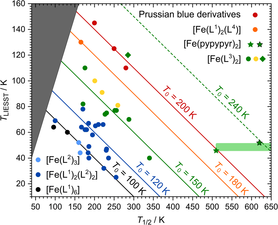 | ||
| Fig. 8 Overview of the T1/2/TLIESST database displayed as established by Létard et al.144,147: data points are assigned to T0 families represented by coloured lines. Since TLIESST cannot be higher than T1/2, there is an area (dark grey) where no data points are to be expected. The colour of the data points indicates the types of ligands in the complexes: six monodentate ligands (black144), two monodentate and two bidentate ligands (dark blue144), three bidentate ligands (light blue144), two tridentate ligands (green,145 yellow,146 green rhombus128), one tetradentate and two monodentate ligands (orange148) and Prussian blue complexes (red149). The new complex [Fe(pypypyr)2] is represented by green stars. Two data points are given: one for the maximum temperature where no spin transition was observed experimentally (510 K) as well as one for the DFT-calculated spin transition temperature (620 K). The area in which the real data point is to be expected is highlighted in light green. | ||
Trying to include [Fe(pypypyr)2] in this database is met with some problems and uncertainties. First of all, Létard et al. defined the following experimental details for the determination of TLIESST: SQUID magnetometric measurements on a sample that is irradiated until saturation and then heated in darkness with a constant heat rate of 0.3 K min−1. In our experiment, we did not reach saturation and used a higher heat rate. Therefore, there can be some uncertainty in the comparability of [Fe(pypypyr)2] with the database. Secondly, [Fe(pypypyr)2] showed no signs of thermal spin transition until 510 K in Mößbauer spectroscopy (see above). Since spin-crossover is more typically investigated below 300 K, the available experimental methods above that temperature are limited. While we did observe a change in the XRPD pattern above 600 K, the data are not clear enough to attribute this change to a spin change. Therefore, we were unable to determine T1/2 experimentally and tried to support the experimental evidence with a theoretical approach. Indeed, using eqn (11) with ΔE0HL = 3300 cm−1 from DFT calculations and ΔS0HL = 5 cm−1 K−1, which is found for many spin-crossover compounds with little variation,40 results in a rough estimate of T1/2 ≈ 620 K for [Fe(pypypyr)2].
Including these data points in the database reveals the remarkable nature of [Fe(pypypyr)2]: while it is expected to be part of the T0 = 150 K family with complexes based on two tridentate ligands, the most conservative data point (T1/2 = 510 K; TLIESST = 46 K) is already on the line of the T0 = 200 K family of Prussian blue derivatives, which is the highest value of T0 observed so far.149 Even more noteable, the DFT-calculated spin transition temperature of 620 K, together with a TLIESST of 52 K, places [Fe(pypypyr)2] in a completely new T0 = 240 K family, well above anything observed so far.
In fact, it is not unprecedented that single complexes do not follow the general trends: while the complex [Fe(bpp(COOH)2)2]2+ is based on tridentate ligands as well, a surprisingly high TLIESST of 120 K was found, placing it into the T0 = 200 K family.128 Indeed, this complex shows astonishingly similar values for ΔΣ and ΔΘ compared to [Fe(pypypyr)2] (see ESI, Table S11†). However, it does not share the asymmetric bond elongation, the low trans-N–Fe–N angle φ and the low bite angles α with [Fe(pypypyr)2] (see ESI, Table S12†). This may explain why [Fe(bpp(COOH)2)2]2+ only shows its exceptional properties in the presence of solvent molecules and turns into an HS compound when dried, whereas [Fe(pypypyr)2] shows its unique behaviour in neat form.
3 Conclusions
In summary, we herein presented the first successful complex syntheses with the ligand bipyridyl pyrrolide (pypypyr−). This monoanionic, tridentate N-donor ligand is topologically related to neutral ligands like terpy or bpp, which have been used to prepare Fe(II) compounds with spin–switchable properties.40,126–128 Our investigation of the spin state using various standard analytical methods revealed that the neutral, vacuum-evaporable complex [Fe(pypypyr)2] has a spin transition temperature above 510 K and thus is a nominal LS complex. Despite that, it still shows the LIESST effect as a neat compound at temperatures below 70 K with an unusually complex relaxation behaviour. The tunneling rate constants determined in three independent experiments are between 10−5 s−1 and 10−2 s−1 and thus four to eleven orders of magnitude lower than expected based on the inverse energy gap law.Careful analysis of single-crystal structures as well as comparison with DFT-calculated structures and structures from the literature show that the unique properties of the title complex are due to a ligand sphere, which induces a LS configuration in the electronic ground state, but enforces distortions along four different types of coordinates upon transition to the metastable HS state: asymmetric Fe–N-bond elongation (parameter ζ), bending of the ligands (parameter ξ), in-plane tilting of the tridentate ligands (parameter φ) and twisting of the two ligands (parameter θ). While other types of Fe(II) complexes (such as [Fe(terpy)2]2+ or [Fe(bpp)2]2+ complexes) also exhibit significant structural distortions, they are not charge neutral (rendering vacuum evaporation difficult) and/or have much lower T1/2 values than the title complex. [Fe(bpp)2]2+ complexes, e.g., are either spin-crossover or even high-spin compounds. Within the limits of the used experimental methods, we found indication that [Fe(pypypyr)2] is at least part of the highest observed T0 family in line with Prussian blue derivatives, but potentially even the first member of a new T0 = 240 K family.
This discovery is of particular interest towards the development of SCO materials with high LIESST temperatures for application in data storage, displays or otherwise. First of all, LS compounds are chemically more robust than HS compounds and thus more suitable for the fabrication of devices. Secondly, TLIESST cannot be higher than T1/2. In order to have LIESST temperatures around 300 K, T1/2 has to exceed that value, implying the use of LS complexes as spin–switchable molecules. While the LIESST temperature of the title complex is not particularly high, it can be increased by modifying the employed ligand. For this, the target ligand would need to maintain the asymmetric structure of bipyridyl pyrrolide and therefore the high structural differences between the two spin states of the resulting complex, while being modified in a way that lowers the spin transition temperature. When T1/2 is low enough, LIESST temperatures of up to 185 K should be possible for molecular complexes. To further increase T0 and thus TLIESST, the demonstrated structural concept may be combined with substituents that increase cooperative interactions, similarly to the results found for [Fe(bpp(COOH)2)2]2+. This way, T0 families around 390 K with LIESST temperatures near room temperature should get within reach.
Author contributions
Jan Grunwald: conceptualization (supporting); data curation; formal analysis (lead); funding acquisition (supporting); investigation (lead); project administration (lead); resources; software; visualization (lead); writing – original draft preparation. Jorge Torres: formal analysis (equal); investigation (equal); visualization (supporting); writing – review & editing (equal). Axel Buchholz: formal analysis (equal); investigation (equal); visualization (supporting). Christian Näther: formal analysis (equal); visualization (supporting); writing – review & editing (equal). Lea Kämmerer: formal analysis (equal); investigation (equal); visualization (supporting); writing – review & editing (equal). Manuel Gruber: funding acquisition (equal); investigation (supporting); writing – review & editing (equal). Sebastian Rohlf: investigation (supporting). Sangeeta Thakur: investigation (supporting). Heiko Wende: funding acquisition (equal); supervision (equal). Winfried Plass: supervision (equal); writing – review & editing (equal). Wolfgang Kuch: formal analysis (supporting); funding acquisition (equal); methodology (equal); project administration (equal); supervision (lead); writing – review & editing (lead). Felix Tuczek: conceptualization (lead); funding acquisition (equal); methodology (equal); project administration (lead); supervision (lead); writing – review & editing (lead).Conflicts of interest
There are no conflicts to declare.Acknowledgements
The authors thank the Deutsche Forschungsgemeinschaft (DFG; TU58/18-1 and KU 1115/13-1) for funding this research. S. Pehlke and J. Pick are acknowledged for Raman, infrared, and CHNS measurements; T. A. Engesser and C. W. A. Trommer, for Mößbauer spectroscopy measurements; D. Meyer, for ESI mass spectrometry measurements; J. Krahmer, M. Höftmann, and G. Kohlmeyer-Yilmaz, for NMR spectroscopy measurements; N. Ruser, P. Hauberg and A. Wolf for XRPD measurements; D. Krause, for DTA/TG measurements; I. Jeß, for X-ray single crystal diffraction, DSC, and XRPD measurements; M. Schmidt for his help with the reparation of a cryostat; and R. Suren for the fabrication of a pneumatic module for the UV/vis spectrometer. NEXAFS measurements were carried out at the VEKMAG station at the BESSY II electron storage ring operated by the Helmholtz-Zentrum Berlin für Materialien und Energie. We would like to thank F. Radu and C. Luo for their assistance during the experiment. The authors thank U. von Hörsten for his expert technical assistance with the Mößbauer measurements at high temperatures. L. K., H. W. and M. G. acknowledge the funding by the Deutsche Forschungsgemeinschaft (DFG; Project-ID 278162697 – CRC 1242, projects A05 and A08).References
- S. Erbas-Cakmak, D. A. Leigh, C. T. McTernan and A. L. Nussbaumer, Chem. Rev., 2015, 115, 10081–10206 CrossRef CAS PubMed.
- S. Kassem, T. Van Leeuwen, A. S. Lubbe, M. R. Wilson, B. L. Feringa and D. A. Leigh, Chem. Soc. Rev., 2017, 46, 2592–2621 RSC.
- I. Aprahamian, ACS Cent. Sci., 2020, 6, 347–358 CrossRef CAS PubMed.
- S. Decurtins, P. Gütlich, C. P. Köhler, H. Spiering and A. Hauser, Chem. Phys. Lett., 1984, 105, 1–4 CrossRef CAS.
- E. Breuning, M. Ruben, J. M. Lehn, F. Renz, Y. Garcia, V. V. Ksenofontov, P. Gütlich, E. Wegelius and K. Rissanen, Angew. Chem., Int. Ed. Engl., 2000, 39, 2504–2507 CrossRef CAS PubMed.
- S. Cobo, G. Molnár, J. A. Real and A. Bousseksou, Angew. Chem., 2006, 118, 5918–5921 CrossRef.
- E. Coronado, J. R. Galán-Mascarós, M. Monrabal-Capilla, J. García-Martínez and P. Pardo-Ibáñez, Adv. Mater., 2007, 19, 1359–1361 CrossRef CAS.
- B. Weber, W. Bauer and J. Obel, Angew. Chem., Int. Ed., 2008, 47, 10098–10101 CrossRef CAS PubMed.
- I. Šalitroš, N. T. Madhu, R. Boča, J. Pavlik and M. Ruben, Monatsh. Chem., 2009, 140, 695–733 CrossRef.
- H. J. Shepherd, G. Molnár, W. Nicolazzi, L. Salmon and A. Bousseksou, Eur. J. Inorg. Chem., 2013, 653–661 CrossRef CAS.
- M. A. Halcrow, Chem. Lett., 2014, 43, 1178–1188 CrossRef CAS.
- G. Molnár, L. Salmon, W. Nicolazzi, F. Terki and A. Bousseksou, J. Mater. Chem. C, 2014, 2, 1360–1366 RSC.
- G. Molnár, S. Rat, L. Salmon, W. Nicolazzi and A. Bousseksou, Adv. Mater., 2018, 30, 1–23 CrossRef PubMed.
- J. Linares, E. Codjovi and Y. Garcia, Sensors, 2012, 12, 4479–4492 CrossRef CAS PubMed.
- C. Bartual-Murgui, A. Akou, C. Thibault, G. Molnár, C. Vieu, L. Salmon and A. Bousseksou, J. Mater. Chem. C, 2015, 3, 1277–1285 RSC.
- C. M. Jureschi, J. Linares, A. Rotaru, M. H. Ritti, M. Parlier, M. M. Dîrtu, M. Wolff and Y. Garcia, Sensors, 2015, 15, 2388–2398 CrossRef CAS PubMed.
- C. M. Jureschi, J. Linares, A. Boulmaali, P. R. Dahoo, A. Rotaru and Y. Garcia, Sensors, 2016, 16, 1–9 CrossRef PubMed.
- K. Boukheddaden, M. H. Ritti, G. Bouchez, M. Sy, M. M. Dîrtu, M. Parlier, J. Linares and Y. Garcia, J. Phys. Chem. C, 2018, 122, 7597–7604 CrossRef CAS.
- B. Benaicha, K. Van Do, A. Yangui, N. Pittala, A. Lusson, M. Sy, G. Bouchez, H. Fourati, C. J. Gómez-Garciá, S. Triki and K. Boukheddaden, Chem. Sci., 2019, 10, 6791–6798 RSC.
- H. J. Shepherd, I. A. Gural'Skiy, C. M. Quintero, S. Tricard, L. Salmon, G. Molnár and A. Bousseksou, Nat. Commun., 2013, 4, 1–9 RSC.
- A. Diaconu, S. L. Lupu, I. Rusu, I. M. Risca, L. Salmon, G. Molnár, A. Bousseksou, P. Demont and A. Rotaru, J. Phys. Chem. Lett., 2017, 8, 3147–3151 CrossRef CAS PubMed.
- O. Kahn, J. Kröber and C. Jay, Adv. Mater., 1992, 4, 718–728 CrossRef CAS.
- Y. Garcia, P. van Koningsbruggen, E. Codjovi, R. Lapouyade, O. Kahn and L. Rabardel, J. Mater. Chem., 1997, 7, 857–858 RSC.
- O. Kahn and C. J. Martinez, Science, 1998, 279, 44–48 CrossRef CAS.
- V. Shalabaeva, K. Ridier, S. Rat, M. D. Manrique-Juarez, L. Salmon, I. Séguy, A. Rotaru, G. Molnár and A. Bousseksou, Appl. Phys. Lett., 2018, 112, 013301 CrossRef.
- G. Hao, A. Mosey, X. Jiang, A. J. Yost, K. R. Sapkota, G. T. Wang, X. Zhang, J. Zhang, A. T. N'Diaye, R. Cheng, X. Xu and P. A. Dowben, Appl. Phys. Lett., 2019, 114, 032901 CrossRef.
- A. Gee, A. H. Jaafar, B. Brachňaková, J. Massey, C. H. Marrows, I. Šalitroš and N. T. Kemp, J. Phys. Chem. C, 2020, 124, 13393–13399 CrossRef CAS.
- Y. Zhang, I. Séguy, K. Ridier, V. Shalabaeva, M. Piedrahita-Bello, A. Rotaru, L. Salmon, G. Molnár and A. Bousseksou, J. Phys.: Condens. Matter, 2020, 32, 1–8 Search PubMed.
- E. P. van Geest, K. Shakouri, W. Fu, V. Robert, V. Tudor, S. Bonnet and G. F. Schneider, Adv. Mater., 2020, 32, 1903575 CrossRef CAS PubMed.
- P. Gütlich, A. Hauser and H. Spiering, Angew. Chem., Int. Ed. Engl., 1994, 33, 2024–2054 CrossRef.
- P. Gütlich, A. B. Gaspar and Y. Garcia, Beilstein J. Org. Chem., 2013, 9, 342–391 CrossRef PubMed.
- P. Gütlich and H. A. Goodwin, in Spin Crossover—An Overall Perspective, ed. P. Gütlich and H. A. Goodwin, Springer Berlin Heidelberg, Berlin, Heidelberg, 2004, pp. 1–47 Search PubMed.
- A. Hauser, in Light-Induced Spin Crossover and the High-Spin → Low-Spin Relaxation, Springer Berlin Heidelberg, Berlin, Heidelberg, 2004, pp. 155–198 Search PubMed.
- J.-F. Létard, P. Guionneau and L. Goux-Capes, in Towards Spin Crossover Applications, Springer Berlin Heidelberg, Berlin, Heidelberg, 2004, pp. 221–249 Search PubMed.
- F. Renz, J. Phys.: Conf. Ser., 2010, 217, 012022 CrossRef.
- D. Unruh, P. Homenya, M. Kumar, R. Sindelar, Y. Garcia and F. Renz, Dalton Trans., 2016, 45, 14008–14018 RSC.
- S. Decurtins, P. Gutlich, K. M. Hasselbach, A. Hauser and H. Spiering, Inorg. Chem., 1985, 24, 2174–2178 CrossRef CAS.
- A. Hauser, Comments Inorg. Chem., 1995, 17, 17–40 CrossRef CAS.
- F. Renz, H. Oshio, V. Ksenofontov, M. Waldeck, H. Spiering and P. Gütlich, Angew. Chem., Int. Ed., 2000, 39, 3699–3700 CrossRef CAS PubMed.
- A. Hauser, C. Enachescu, M. L. Daku, A. Vargas and N. Amstutz, Coord. Chem. Rev., 2006, 250, 1642–1652 CrossRef CAS.
- J. S. Costa, C. Balde, C. Carbonera, D. Denux, A. Wattiaux, C. Desplanches, J. P. Ader, P. Gütlich and J. F. Létard, Inorg. Chem., 2007, 46, 4114–4119 CrossRef PubMed.
- R. Ababei, C. Pichon, O. Roubeau, Y. G. Li, N. Bréfuel, L. Buisson, P. Guionneau, C. Mathonière and R. Clérac, J. Am. Chem. Soc., 2013, 135, 14840–14853 CrossRef CAS PubMed.
- H. Wang, C. Desplanches, P. Dagault and J. F. Létard, Dalton Trans., 2014, 43, 15346–15350 RSC.
- D. Aguilà, P. Dechambenoit, M. Rouzières, C. Mathonière and R. Clérac, Chem. Commun., 2017, 53, 11588–11591 RSC.
- Z. S. Yao, Z. Tang and J. Tao, Chem. Commun., 2020, 56, 2071–2086 RSC.
- M. Ruben and K. S. Kumar, Angew. Chem., Int. Ed., 2019, 60, 7502–7521 Search PubMed.
- M. Gruber and R. Berndt, Magnetochemistry, 2020, 6, 35 CrossRef CAS.
- L. Kipgen, M. Bernien, F. Tuczek and W. Kuch, Adv. Mater., 2021, 33, 2008141 CrossRef CAS PubMed.
- M. Cavallini, Phys. Chem. Chem. Phys., 2012, 14, 11867–11876 RSC.
- T. Mallah and M. Cavallini, C. R. Chim., 2018, 21, 1270–1286 CrossRef CAS.
- C. Thibault, G. Moinár, L. Salmon, A. Bousseksou and C. Vieu, Langmuir, 2010, 26, 1557–1560 CrossRef CAS PubMed.
- S. Basak, P. Hui and R. Chandrasekar, Chem. Mater., 2013, 25, 3408–3413 CrossRef CAS.
- U. Venkataramudu, S. Basak, M. A. Mohiddon and R. Chandrasekar, J. Chem. Sci., 2018, 130, 1–6 CrossRef CAS.
- M. L. Boillot, C. Roux, J. P. Audière, A. Dausse and J. Zarembowitch, Inorg. Chem., 1996, 35, 3975–3980 CrossRef CAS PubMed.
- K. Kuroiwa, T. Shibata, S. Sasaki, M. Ohba, A. Takahara, T. Kunitake and N. Kimizuka, J. Polym. Sci., Part A: Polym. Chem., 2006, 44, 5192–5202 CrossRef CAS.
- M. Matsuda and H. Tajima, Chem. Lett., 2007, 36, 700–701 CrossRef CAS.
- M. Matsuda, H. Isozaki and H. Tajima, Thin Solid Films, 2008, 517, 1465–1467 CrossRef CAS.
- A. Tissot, J. F. Bardeau, E. Rivière, F. Brisset and M. L. Boillot, Dalton Trans., 2010, 39, 7806–7812 RSC.
- E. M. Hernández, C. M. Quintero, O. Kraieva, C. Thibault, C. Bergaud, L. Salmon, G. Molnár and A. Bousseksou, Adv. Mater., 2014, 26, 2889–2893 CrossRef PubMed.
- H. Soyer, C. Mingotaud, M. L. Boillot and P. Delhaes, Langmuir, 1998, 14, 5890–5894 CrossRef CAS.
- J. F. Létard, O. Nguyen, H. Soyer, C. Mingotaud, P. Delhaès and O. Kahn, Inorg. Chem., 1999, 38, 3020–3021 CrossRef.
- O. Roubeau, B. Agricole, R. Clérac and S. Ravaine, J. Phys. Chem. B, 2004, 108, 15110–15116 CrossRef CAS.
- J. A. Kitchen, N. G. White, C. Gandolfi, M. Albrecht, G. N. Jameson, J. L. Tallon and S. Brooker, Chem. Commun., 2010, 46, 6464–6466 RSC.
- P. N. Martinho, I. A. Kühne, B. Gildea, G. McKerr, B. O'hagan, T. E. Keyes, T. Lemma, C. Gandolfi, M. Albrecht and G. G. Morgan, Magnetochemistry, 2018, 4, 1–16 CrossRef.
- T. Jasper-Tönnies, M. Gruber, S. Karan, H. Jacob, F. Tuczek and R. Berndt, J. Phys. Chem. Lett., 2017, 8, 1569–1573 CrossRef PubMed.
- T. Knaak, C. González, Y. J. Dappe, G. D. Harzmann, T. Brandl, M. Mayor, R. Berndt and M. Gruber, J. Phys. Chem. C, 2019, 123, 4178–4185 CrossRef CAS.
- T. Brandl, S. Johannsen, D. Häussinger, N. Suryadevara, A. Prescimone, S. Bernhard, M. Gruber, M. Ruben, R. Berndt and M. Mayor, Angew. Chem., Int. Ed., 2020, 59, 15947–15952 CrossRef CAS PubMed.
- S. Shi, G. Schmerber, J. Arabski, J.-B. Beaufrand, D. J. Kim, S. Boukari, M. Bowen, N. T. Kemp, N. Viart, G. Rogez, E. Beaurepaire, H. Aubriet and J. Petersen, Appl. Phys. Lett., 2009, 95, 43303 CrossRef.
- T. Miyamachi, M. Gruber, V. Davesne, M. Bowen, S. Boukari, L. Joly, F. Scheurer, G. Rogez, T. K. Yamada, P. Ohresser, E. Beaurepaire and W. Wulfhekel, Nat. Commun., 2012, 3, 938 CrossRef PubMed.
- M. Gruber, V. Davesne, M. Bowen, S. Boukari, E. Beaurepaire, W. Wulfhekel and T. Miyamachi, Phys. Rev. B: Condens. Matter Mater. Phys., 2014, 89, 1–9 CrossRef.
- S. Gueddida, M. Gruber, T. Miyamachi, E. Beaurepaire, W. Wulfhekel and M. Alouani, J. Phys. Chem. Lett., 2016, 7, 900–904 CrossRef CAS PubMed.
- S. Beniwal, S. Sarkar, F. Baier, B. Weber, P. A. Dowben and A. Enders, J. Phys.: Condens. Matter, 2020, 32, 1–6 CrossRef PubMed.
- H. Naggert, A. Bannwarth, S. Chemnitz, T. v. Hofe, E. Quandt and F. Tuczek, Dalton Trans., 2011, 40, 6364–6366 RSC.
- T. G. Gopakumar, F. Matino, H. Naggert, A. Bannwarth, F. Tuczek and R. Berndt, Angew. Chem., Int. Ed., 2012, 51, 6262–6266 CrossRef CAS PubMed.
- T. Palamarciuc, J. C. Oberg, F. El Hallak, C. F. Hirjibehedin, M. Serri, S. Heutz, J. F. Létard and P. Rosa, J. Mater. Chem., 2012, 22, 9690–9695 RSC.
- A. Pronschinske, R. C. Bruce, G. Lewis, Y. Chen, A. Calzolari, M. Buongiorno-Nardelli, D. A. Shultz, W. You and D. B. Dougherty, Chem. Commun., 2013, 49, 10446–10452 RSC.
- B. Warner, J. C. Oberg, T. G. Gill, F. El Hallak, C. F. Hirjibehedin, M. Serri, S. Heutz, M. A. Arrio, P. Sainctavit, M. Mannini, G. Poneti, R. Sessoli and P. Rosa, J. Phys. Chem. Lett., 2013, 4, 1546–1552 CrossRef CAS PubMed.
- H. Naggert, J. Rudnik, L. Kipgen, M. Bernien, F. Nickel, L. M. Arruda, W. Kuch, C. Näther and F. Tuczek, J. Mater. Chem. C, 2015, 3, 7870–7877 RSC.
- L. Kipgen, M. Bernien, S. Ossinger, F. Nickel, A. J. Britton, L. M. Arruda, H. Naggert, C. Luo, C. Lotze, H. Ryll, F. Radu, E. Schierle, E. Weschke, F. Tuczek and W. Kuch, Nat. Commun., 2018, 9, 1–8 CrossRef CAS PubMed.
- S. Ossinger, L. Kipgen, H. Naggert, M. Bernien, A. J. Britton, F. Nickel, L. M. Arruda, I. Kumberg, T. A. Engesser, E. Golias, C. Näther, F. Tuczek and W. Kuch, J. Phys.: Condens. Matter, 2020, 32, 114003 CrossRef CAS PubMed.
- T. Mahfoud, G. Molnár, S. Cobo, L. Salmon, C. Thibault, C. Vieu, P. Demont and A. Bousseksou, Appl. Phys. Lett., 2011, 99, 1–4 CrossRef.
- V. Davesne, M. Gruber, M. Studniarek, W. H. Doh, S. Zafeiratos, L. Joly, F. Sirotti, M. G. Silly, A. B. Gaspar, J. A. Real, G. Schmerber, M. Bowen, W. Weber, S. Boukari, V. Da Costa, J. Arabski, W. Wulfhekel and E. Beaurepaire, J. Chem. Phys., 2015, 142, 194702 CrossRef CAS PubMed.
- V. Shalabaeva, M. Mikolasek, M. D. Manrique-Juarez, A. C. Bas, S. Rat, L. Salmon, W. Nicolazzi, G. Molnár and A. Bousseksou, J. Phys. Chem. C, 2017, 121, 25617–25621 CrossRef CAS.
- V. Shalabaeva, S. Rat, M. D. Manrique-Juarez, A.-C. Bas, L. Vendier, L. Salmon, G. Molnár and A. Bousseksou, J. Mater. Chem. C, 2017, 5, 4419–4425 RSC.
- K. Bairagi, A. Bellec, C. Fourmental, O. Iasco, J. Lagoute, C. Chacon, Y. Girard, S. Rousset, F. Choueikani, E. Otero, P. Ohresser, P. Sainctavit, M. L. Boillot, T. Mallah and V. Repain, J. Phys. Chem. C, 2018, 122, 727–731 CrossRef CAS.
- A. C. Bas, V. Shalabaeva, X. Thompson, L. Vendier, L. Salmon, C. Thibault, G. Molnár, L. Routaboul and A. Bousseksou, C. R. Chim., 2019, 22, 525–533 CrossRef CAS.
- C. Fourmental, S. Mondal, R. Banerjee, A. Bellec, Y. Garreau, A. Coati, C. Chacon, Y. Girard, J. Lagoute, S. Rousset, M. L. Boillot, T. Mallah, C. Enachescu, C. Barreteau, Y. J. Dappe, A. Smogunov, S. Narasimhan and V. Repain, J. Phys. Chem. Lett., 2019, 10, 4103–4109 CrossRef CAS PubMed.
- K. Ridier, A. C. Bas, V. Shalabaeva, W. Nicolazzi, L. Salmon, G. Molnár, A. Bousseksou, M. Lorenc, R. Bertoni, E. Collet and H. Cailleau, Adv. Mater., 2019, 31, 1–7 CrossRef PubMed.
- K. Ridier, Y. Zhang, M. Piedrahita-Bello, C. M. Quintero, L. Salmon, G. Molnár, C. Bergaud and A. Bousseksou, Adv. Mater., 2020, 32, 1–5 CrossRef PubMed.
- L. Zhang, Y. Tong, M. Kelai, A. Bellec, J. Lagoute, C. Chacon, Y. Girard, S. Rousset, M. L. Boillot, E. Rivière, T. Mallah, E. Otero, M. A. Arrio, P. Sainctavit and V. Repain, Angew. Chem., Int. Ed., 2020, 59, 13341–13346 CrossRef CAS PubMed.
- M. Atzori, L. Poggini, L. Squillantini, B. Cortigiani, M. Gonidec, P. Bencok, R. Sessoli and M. Mannini, J. Mater. Chem. C, 2018, 6, 8885–8889 RSC.
- M. Bernien, D. Wiedemann, C. F. Hermanns, A. Krüger, D. Rolf, W. Kroener, P. Müller, A. Grohmann and W. Kuch, J. Phys. Chem. Lett., 2012, 3, 3431–3434 CrossRef CAS PubMed.
- S. Rohlf, M. Gruber, B. M. Flöser, J. Grunwald, S. Jarausch, F. Diekmann, M. Kalläne, T. Jasper-Toennies, A. Buchholz, W. Plass, R. Berndt, F. Tuczek and K. Rossnagel, J. Phys. Chem. Lett., 2018, 9, 1491–1496 CrossRef CAS PubMed.
- T. G. Gopakumar, M. Bernien, H. Naggert, F. Matino, C. F. Hermanns, A. Bannwarth, S. Mühlenberend, A. Krüger, D. Krüger, F. Nickel, W. Walter, R. Berndt, W. Kuch and F. Tuczek, Chem. – Eur. J., 2013, 19, 15702–15709 CrossRef CAS PubMed.
- S. Ossinger, H. Naggert, L. Kipgen, T. Jasper-Tönnies, A. Rai, J. Rudnik, F. Nickel, L. M. Arruda, M. Bernien, W. Kuch, R. Berndt and F. Tuczek, J. Phys. Chem. C, 2017, 121, 1210–1219 CrossRef CAS.
- S. Rohlf, J. Grunwald, T. Jasper-Tönnies, S. Johannsen, F. Diekmann, M. Studniarek, R. Berndt, F. Tuczek, K. Rossnagel and M. Gruber, J. Phys. Chem. C, 2019, 123, 17774–17780 CrossRef CAS.
- K. Bairagi, O. Iasco, A. Bellec, A. Kartsev, D. Li, J. Lagoute, C. Chacon, Y. Girard, S. Rousset, F. Miserque, Y. J. Dappe, A. Smogunov, C. Barreteau, M.-L. Boillot, T. Mallah and V. Repain, Nat. Commun., 2016, 7, 12212 CrossRef CAS PubMed.
- S. Johannsen, S. Ossinger, T. Markussen, F. Tuczek, M. Gruber and R. Berndt, ACS Nano, 2021, 15, 11770–11778 CrossRef CAS PubMed.
- M. Böttger, B. Wiegmann, S. Schaumburg, P. G. Jones, W. Kowalsky and H. H. Johannes, Beilstein J. Org. Chem., 2012, 8, 1037–1047 CrossRef PubMed.
- Z. Z. Sun, K. M. Zheng, Q. S. Li and Z. S. Li, RSC Adv., 2014, 4, 31544–31551 RSC.
- T. Nagata and K. Tanaka, Bull. Chem. Soc. Jpn., 2002, 75, 2469–2470 CrossRef CAS.
- A. Bhattacharjee, H. A. Goodwin and P. Gütlich, AIP Conf. Proc., 2010, 1313, 128–130 CrossRef CAS.
- G. J. Long and B. B. Hutchinson, Inorg. Chem., 1987, 26, 608–613 CrossRef CAS.
- M. Seredyuk, A. B. Gaspar, J. Kusz, G. Bednarek and P. Gütlich, J. Appl. Crystallogr., 2007, 40, 1135–1145 CrossRef CAS.
- S. Ossinger, C. Näther, A. Buchholz, M. Schmidtmann, S. Mangelsen, R. Beckhaus, W. Plass and F. Tuczek, Inorg. Chem., 2020, 59, 7966–7979 CrossRef CAS PubMed.
- N. Suryadevara, A. Mizuno, L. Spieker, S. Salamon, S. Sleziona, A. Maas, E. Pollmann, B. Heinrich, M. Schleberger, H. Wende, S. K. Kuppusamy and M. Ruben, Chem. – Eur. J., 2022, 28, e202103853 CAS.
- G. Chastanet, C. Desplanches, C. Baldé, P. Rosa, M. Marchivie and P. Guionneau, Chem. Sq., 2018, 2, 2 Search PubMed.
- W. Szczerba, M. Schott, H. Riesemeier, A. F. Thünemann and D. G. Kurth, Phys. Chem. Chem. Phys., 2014, 16, 19694–19701 RSC.
- N. Shi, Q. Gao, A. Sanson, Q. Li, L. Fan, Y. Ren, L. Olivi, J. Chen and X. Xing, Dalton Trans., 2019, 48, 3658–3663 RSC.
- A. T. Baker and H. A. Goodwin, Aust. J. Chem., 1985, 38, 207–214 CrossRef CAS.
- L. A. Barrios, C. Bartual-Murgui, E. Peyrecave-Lleixà, B. Le Guennic, S. J. Teat, O. Roubeau and G. Aromí, Inorg. Chem., 2016, 55, 4110–4116 CrossRef CAS PubMed.
- A. Hauser, Chem. Phys. Lett., 1986, 124, 543–548 CrossRef CAS.
- A. Hauser, J. Chem. Phys., 1991, 94, 2741–2748 CrossRef CAS.
- S. Schenker, A. Hauser and R. M. Dyson, Inorg. Chem., 1996, 35, 4676–4682 CrossRef CAS.
- M. Bernien, H. Naggert, L. M. Arruda, L. Kipgen, F. Nickel, J. Miguel, C. F. Hermanns, A. Krüger, D. Krüger, E. Schierle, E. Weschke, F. Tuczek and W. Kuch, ACS Nano, 2015, 9, 8960–8966 CrossRef CAS PubMed.
- M. Gruber, T. Miyamachi, V. Davesne, M. Bowen, S. Boukari, W. Wulfhekel, M. Alouani and E. Beaurepaire, J. Chem. Phys., 2017, 146, 092312 CrossRef.
- D. Collison, C. David Garner, C. M. McGrath, J. F. W. Mosselmans, M. D. Roper, J. M. W. Seddon, E. Sinn and N. A. Young, J. Chem. Soc., Dalton Trans., 1997, 4371–4376 RSC.
- V. Davesne, M. Gruber, T. Miyamachi, V. Da Costa, S. Boukari, F. Scheurer, L. Joly, P. Ohresser, E. Otero, F. Choueikani, A. B. Gaspar, J. A. Real, W. Wulfhekel, M. Bowen and E. Beaurepaire, J. Chem. Phys., 2013, 139, 74708 CrossRef CAS PubMed.
- L. Kipgen, M. Bernien, F. Nickel, H. Naggert, A. J. Britton, L. M. Arruda, E. Schierle, E. Weschke, F. Tuczek and W. Kuch, J. Phys.: Condens. Matter, 2017, 29, 394003 CrossRef PubMed.
- E. Ludwig, H. Naggert, M. Kalläne, S. Rohlf, E. Kröger, A. Bannwarth, A. Quer, K. Rossnagel, L. Kipp and F. Tuczek, Angew. Chem., 2014, 126, 3063–3067 CrossRef.
- E. Buhks, G. Navon, M. Bixon and J. Jortner, J. Am. Chem. Soc., 1980, 102, 2918–2923 CrossRef CAS.
- J. Kusz, H. Spiering and P. Gütlich, J. Appl. Crystallogr., 2000, 33, 201–205 CrossRef CAS.
- J. Kusz, H. Spiering and P. Gütlich, J. Appl. Crystallogr., 2001, 34, 229–238 CrossRef CAS.
- J. A. Real, M. C. Muñoz, J. Faus and X. Solans, Inorg. Chem., 1997, 36, 3008–3013 CrossRef CAS PubMed.
- S. Ossinger, C. Näther and F. Tuczek, Acta Crystallogr., Sect. E: Crystallogr. Commun., 2019, 75, 1112–1116 CrossRef CAS PubMed.
- J. M. Holland, J. A. McAllister, C. A. Kilner, M. Thornton-Pett, A. J. Bridgeman and M. A. Halcrow, J. Chem. Soc., Dalton Trans., 2002, 2, 548–554 RSC.
- L. J. Kershaw Cook, F. L. Thorp-Greenwood, T. P. Comyn, O. Cespedes, G. Chastanet and M. A. Halcrow, Inorg. Chem., 2015, 54, 6319–6330 CrossRef CAS PubMed.
- V. García-López, M. Palacios-Corella, S. Cardona-Serra, M. Clemente-León and E. Coronado, Chem. Commun., 2019, 55, 12227–12230 RSC.
- M. A. Halcrow, Coord. Chem. Rev., 2009, 253, 2493–2514 CrossRef CAS.
- S. Vela, J. J. Novoa and J. Ribas-Arino, Phys. Chem. Chem. Phys., 2014, 16, 27012–27024 RSC.
- L. J. Cook, R. Kulmaczewski, O. Cespedes and M. A. Halcrow, Chem. – Eur. J., 2016, 22, 1789–1799 CrossRef CAS PubMed.
- K. Senthil Kumar, B. Heinrich, S. Vela, E. Moreno-Pineda, C. Bailly and M. Ruben, Dalton Trans., 2019, 48, 3825–3830 RSC.
- P. Guionneau, M. Marchivie, G. Bravic, J.-F. Létard and D. Chasseau, in Structural Aspects of Spin Crossover. Example of the [FeIILn(NCS)2] Complexes, Springer Berlin Heidelberg, Berlin, Heidelberg, 2004, pp. 97–128 Search PubMed.
- M. Marchivie, P. Guionneau, J. F. Létard and D. Chasseau, Acta Crystallogr., Sect. B: Struct. Sci., Cryst. Eng. Mater., 2005, 61, 25–28 CrossRef PubMed.
- R. Ketkaew, Y. Tantirungrotechai, P. Harding, G. Chastanet, P. Guionneau, M. Marchivie and D. J. Harding, Dalton Trans., 2021, 50, 1086–1096 RSC.
- C. Boilleau, N. Suaud and N. Guihéry, J. Chem. Phys., 2012, 137, 224304 CrossRef PubMed.
- A. Hauser, Chem. Phys. Lett., 1992, 192, 65–70 CrossRef CAS.
- O. Roubeau, J. G. Haasnoot, J. Linarès and F. Varret, Mol. Cryst. Liq. Cryst. Sci. Technol., Sect. A, 1999, 335, 541–550 CrossRef.
- C. Enachescu, J. Linares, F. Varret, K. Boukheddaden, E. Codjovi, S. G. Salunke and R. Mukherjee, Inorg. Chem., 2004, 43, 4880–4888 CrossRef CAS PubMed.
- Y. Ogawa, S. Koshihara, K. Koshino, T. Ogawa, C. Urano and H. Takagi, Phys. Rev. Lett., 2000, 84, 3181–3184 CrossRef CAS PubMed.
- C. Enachescu, H. Constant-Machado, E. Codjovi, J. Linares, K. Boukheddaden and F. Varret, J. Phys. Chem. Solids, 2001, 62, 1409–1422 CrossRef CAS.
- C. Enachescu, U. Oetliker and A. Hauser, J. Phys. Chem. B, 2002, 106, 9540–9545 CrossRef CAS.
- R. Bertoni, M. Cammarata, M. Lorenc, S. F. Matar, J. F. Létard, H. T. Lemke and E. Collet, Acc. Chem. Res., 2015, 48, 774–781 CrossRef CAS PubMed.
- J. F. Létard, L. Capes, G. Chastanet, N. Moliner, S. Létard, J. A. Real and O. Kahn, Chem. Phys. Lett., 1999, 313, 115–120 CrossRef.
- S. Marcén, L. Lecren, L. Capes, H. A. Goodwin and J.-F. Létard, Chem. Phys. Lett., 2002, 358, 87–95 CrossRef.
- V. A. Money, J. S. Costa, S. Marcén, G. Chastanet, J. Elhaïk, M. A. Halcrow, J. A. K. Howard and J.-F. Létard, Chem. Phys. Lett., 2004, 391, 273–277 CrossRef CAS.
- J.-F. Létard, P. Guionneau, O. Nguyen, J. S. Costa, S. Marcén, G. Chastanet, M. Marchivie and L. Goux-Capes, Chem. – Eur. J., 2005, 11, 4582–4589 CrossRef PubMed.
- S. Hayami, Z.-z. Gu, Y. Einaga, Y. Kobayasi, Y. Ishikawa, Y. Yamada, A. Fujishima and O. Sato, Inorg. Chem., 2001, 40, 3240–3242 CrossRef CAS PubMed.
- N. Shimamoto, S.-i. Ohkoshi, O. Sato and K. Hashimoto, Inorg. Chem., 2002, 41, 678–684 CrossRef CAS PubMed.
Footnote |
| † Electronic supplementary information (ESI) available: Experimental details of the syntheses and analytical methods, additional data and explanation of the data evaluation for the presented analytical methods, Mößbauer spectra, FIR spectra, resonance Raman spectra, DFT and crystal structure data. CCDC 2233051 and 2233052. For ESI and crystallographic data in CIF or other electronic format see DOI: https://doi.org/10.1039/d3sc00561e |
| This journal is © The Royal Society of Chemistry 2023 |